npTrack: A n-Position Single Axis Solar Tracker Model for Optimized Energy Collection

Abstract

The single axis solar tracker based on flat panels is used in large solar plants and in distribution-level photovoltaic systems. In order to achieve this, the solar tracking systems generally need to work by tracking the sun’s position with dozens, maybe hundreds of movements along the day with a maximal known tracking error within the specifications. A novel model is proposed along this work based on the control of the angle deviation within a (polar) single axis configuration. This way an optimization of the harnessing of solar energy can be achieved with as few panel displacements as possible in order to decrease the wear in the mechanical parts of the equipment and the energy consumed by it. This tracking approach was implemented with as few as seven positions along the day and got an estimated theoretical value of 99.27% of the total collected energy in a continuous tracking system. Regarding an annual average basis, it would be about 96.5% of a dual axis system according to the proposed model. The novelty of the model is related to a tradeoff between the gain with the simplicity of a single axis n-position tracking and the solar energy loss associated.

1. Introduction

To increase the collected energy regarding direct irradiance, the need to move the photovoltaic panels to get them perpendicular to sun rays has led to hundreds of tracking devices. During the past few decades, some important differences have been pointed out about the solar tracking systems in relation to the tracking geometry used, the working mechanics and their associated electrical and electronic parts. Reviews and comparisons about these technologies have been made in the past, as can be found in the article by Mousazadeh [1] in 2009, that depicted detailed information about the main solar tracking solutions used at the time.

Since then, the research has brought new concepts and tested new solutions, which can be found in the paper of Seme that presents an updated scenario [2]. The manufacturers have also continued to develop their technologies, each one with its specific tracking error, that is, the deviation of the angle between the sun ray and the normal of the photovoltaic panel, which should be as low as possible as a function of the chosen geometry and electromechanical parts involved. In order to get this best condition, continuous tracking movement is performed by the electromechanical apparatus to update its position with time. By continuous, sometimes it can be understood as it moves slowly in small steps within small time intervals. It can be, for instance, 4 min or less, depending on the precision required by the tracker equipment specification. In other designs, as happens when the rotation start/stop signal comes from the output of light sensors separated by a barrier (that produces shadow with the relative sun movement), the “continuous movement” means that the interval time is a response of such a shadowing scheme and its control electronics behind. In the article of Ponniran [3], by instance, that barrier scheme to adjust the position of the tracker was used with light dependent resistors, or LDRs, a kind of photosensor. In a more recent paper, Kuttybay compared the use of a LDR photosensor with a scheduled scheme by using an encoder sensor to measure the angle shift and the displacement needed to track the azimuth angle of the sun [4]. That study concluded that such an approach was 4.2% more efficient than using a LDR solar tracker in different weather conditions. According to the results, the authors expected to get an increase of 37% in total long term power generation when compared to a fixed photovoltaic (PV) panel in a region with high solar resources. In addition to LDRs, photodiodes have been used as an optical sensor option to correct and adjust the position in solar trackers. The work of Zhang, for instance, used photodiodes in a dual-axis hybrid solar track system, which also uses a GPS module [5]. As another more recent alternative, the inclinometer, a device designed to measure the angle of an object with respect to the force of gravity, also called the tilt sensor, has been used in order to adjust the position of the PV panels adopted according to the model and geometry adopted [2].

Solar trackers based on a few discrete positions along the day were also targeted in some approaches. The work of Abdallah is an example of a discrete tracking system based on four positions in a vertical axis (V-axis mount), regarded the solar azimuth change along the day [6]. According to the authors, the productivity was increased for around 22%, with an overall efficiency increase of about 2%. The research of Huang also was made by using a discrete tracking system rotating around a vertical axis, but with three positions instead [7]. Compared to an identical, but fixed assembly, the approach managed to increase the solar energy collected on a sunny day by 34.6%. The study of Batayneha was also based on three positions throughout the day with respect to the azimuth plane to follow the sun [8], so that the discrete tracking approach managed to obtain about 91–94% of the energy that would be collected in the case of a continuous solar tracking mode. In another article, Zhong led a theoretical study to analyze a tracking system with an inclined south–north axis (ISNA) [9]. That approach used three tracking positions along the day. Moreover, it was yearly adjusted 4 times at three fixed tilted angles related to the south–north inclination. The maximum collectible annual radiation was about 96% in comparison to a 2-axis tracker. Li, in another approach, developed a research using mathematical procedures to estimate the annual collectible radiation on fixed and tracked panels based on solar geometry and monthly horizontal radiation [10]. The research found that the maximum annual collectible radiation on ISNA-axis tracked panels was about 97–98% of that on dual-axis tracked panels, while the same study showed a result above 99% of that on dual-axis tracked panels with the tilt angle of the ISNA being yearly adjusted four times at three yearly fixed positions. Zhu, by its time, designed a single axis solar tracking structure, called tilted-rotating axis tracking (TR-axis tracking) [11]. Computer simulations revealed that the TR-axis tracking was able to collect 96.4% of the solar energy received in a dual-axis system. Bahrami led a research about the latitude effects on the performance of different solar trackers in Europe and Africa and concluded that ISNA type solar trackers have better performance than vertical-axis solar trackers in latitudes below 26° [12]. An anisotropic sky diffuse model was regarded to predict the available potential of each location.

In brief, currently there are continuous and n-positions solar trackers that, in fact, behave in steps when moving. The key point about the maximum admissible tracking error between those approaches and their consequences on the final collected solar energy can help to choose and project such systems. It is worth to note that the more tracking accuracy is required, the shorter time intervals are needed, which also demands more accurate devices included in the subsystems as sensors, motors or actuators, gears, timers, etc. Additionally, it will result in more collected energy according to a cost/benefit ratio.

Regarding a PV system for a commercial or even for a utility scale use, the determination of the tracking system should take several costs into account: land, equipment and maintenance, for instance. On the other hand, the complexity of a dual-axis tracking was an important aspect brought to light in a study done by Martin [13]. That article also found that such complexity was underestimated by comparing the design of a dual-axis tracking power plant to another five PV plants in Spain. Another comparison took place among several solar trackers, the case study led by Bahrami in Nigeria (latitudes between 4 and 14° N) that analyzed nine locations with fixed, single and dual-axis solar tracking PV systems [14]. Based on an indicator of technical and economic feasibility, called levelized cost of electricity (LCOE), the study concluded from the results obtained in Nigeria that the single axis tracking is more advantageous than dual axis tracking when the total PV system installation cost is relatively low. In addition, an east–west tracker was a preferred option for implementation followed by the two inclined (including one optimized) east–west trackers. Moreover, the results can be applied for 21 low latitudes (0–15° N) countries. In another article [15], Bahrami concluded that, for any given latitude, as the PV installation costs increases, the full axis and vertical (optimized) trackers become more advantageous, the opposite of what happens to the east–west and north–south trackers. Additionally, as the latitude increases in the northern hemisphere, the east–west trackers move down in the rank and both, the vertical (optimized) and the north–south trackers, move up in the rank regardless of the PV system installation costs. In addition, for latitudes between 25 and 45° N with higher solar irradiation level, the vertical optimized and inclined east–west optimized trackers perform better than north–south/east–west tracking in locations.

The focus in this work was evaluating the energy output of a single axis polar mount tracking system (without concentration) when the tracking error is conveniently increased according to strategies created to accomplish their tasks. That was also a search for advantages of a tracking strategy design, such as simplicity allied with robustness, when conceived with more tolerance to positioning deviation. A solar tracker built simpler allows not only robustness, but means cost savings in terms of the equipment price and the maintenance services. In fact, the previous references showed that a less expensive single axis east–west tracker can be commercial feasible to be deployed in higher latitudes. According to the work of D’Adamo [16], the post Covid-19 can bring favorable scenarios to employ solar energy technologies in residential plants in Italy, presumably an opportunity to use cheaper and simpler electromechanical systems with few tracking positions a day. In another economic analysis due to D’Adamo, in the recent years the PV technology has become progressively affordable not only due to efficiency gains, but in terms of the solar energy production costs [17]. In order to optimize the gains, it is worth to mention the work of Rehman, which performed a study about the performance through optimal geometries in a search for the best positioning photovoltaic arrays in a constrained field [18]. Regarding this whole context, the novelty is proposed along this text through a model that deals about how to simplify the electromechanical solar tracking system, which is translated into cost reduction in operation/maintenance of a single axis solar tracker. At the same time, it is offered ways to minimize, by the adequate choose of the number of discrete positions, the loss of the collected solar energy in a single axis polar mount.

2. Materials and Methods

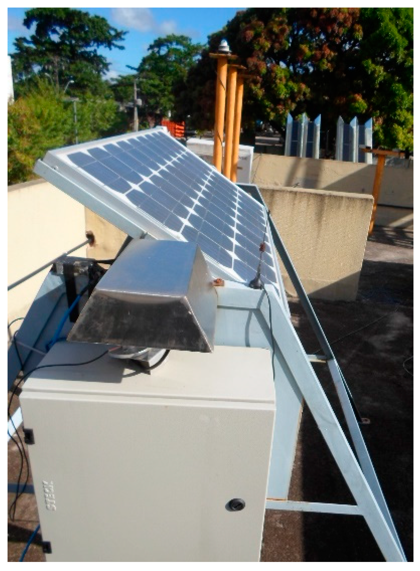
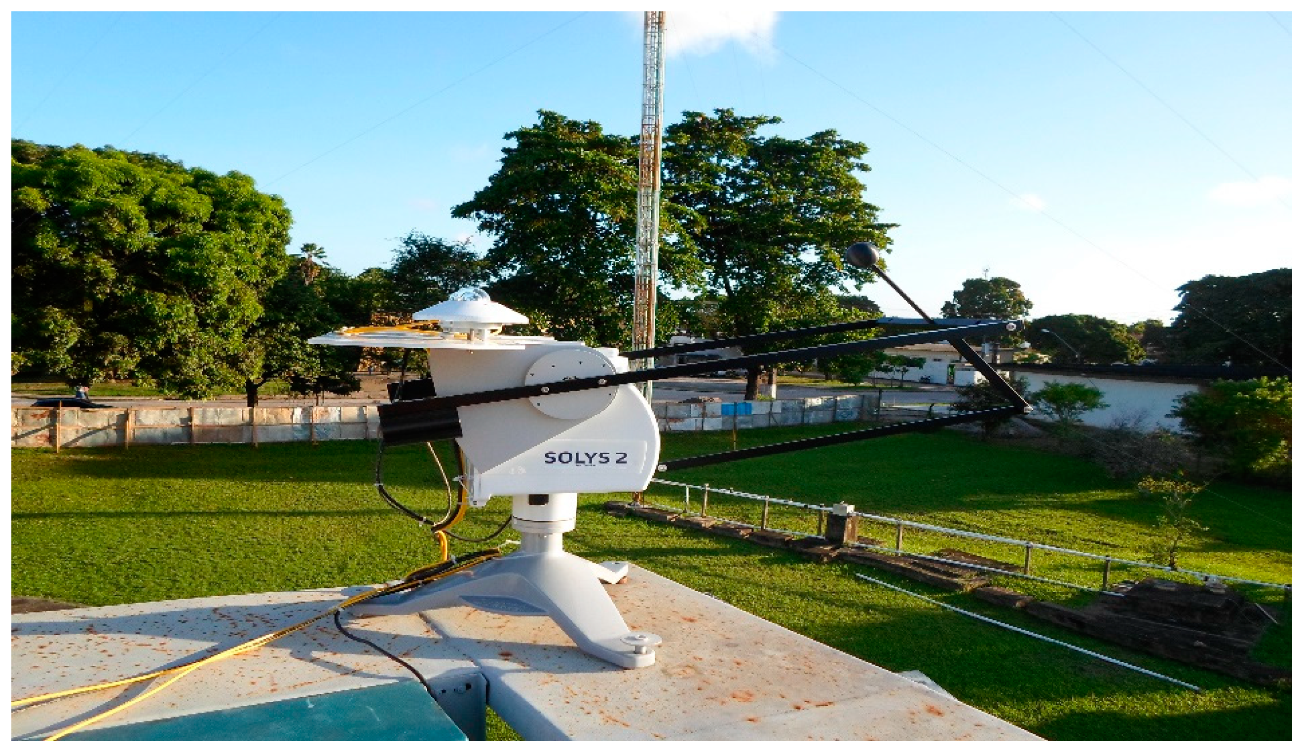
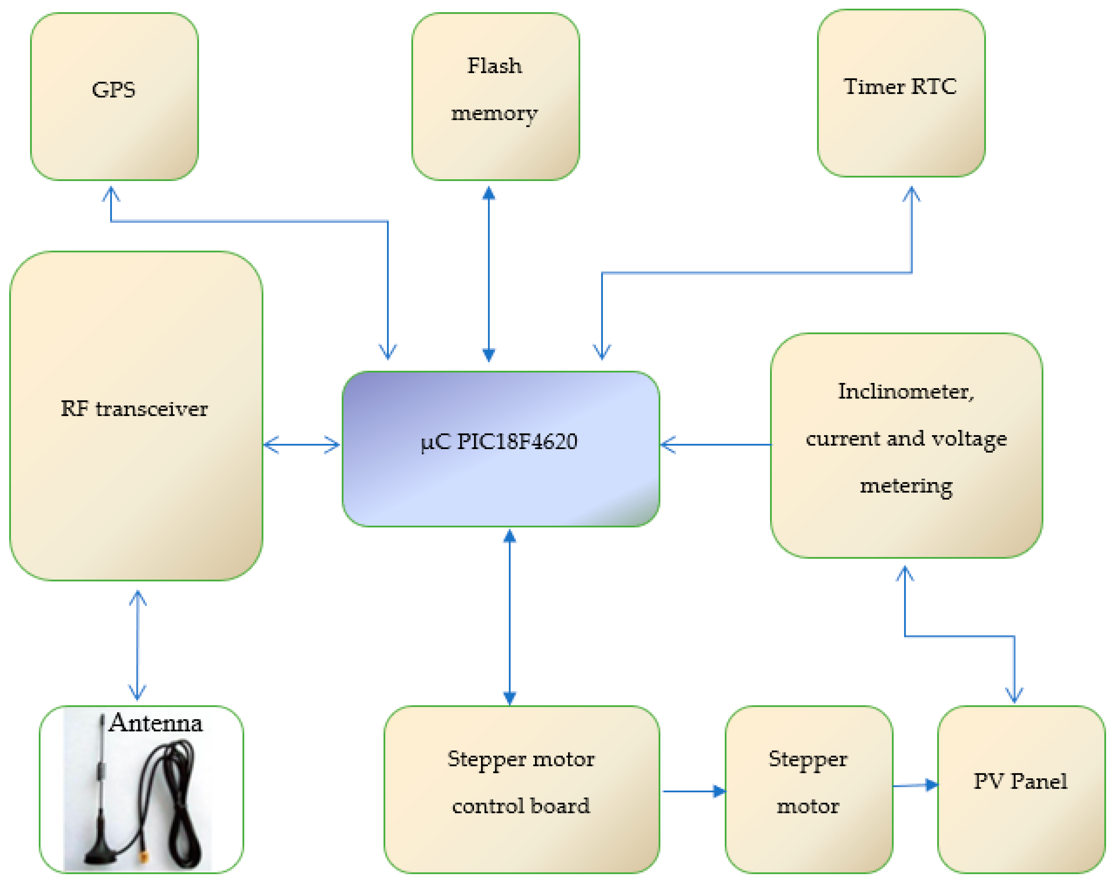
As a project concept, a multitracker system was adopted within a (remotely) supervised-module architecture. The role of processing the most complex data is done by the software in a desktop computer, which controls the tracker through the firmware setup. On the other hand, the tracker module, Figure 1, was in charge of rotating the PV panel built within a polar geometry, where the axis tilt is the latitude of the local, following the movement of the sun (east–west) while storing the energy collected as output of three previously conceived tracking strategies. That task was done with the help of a microcontroller (PIC18F4620) and its firmware that handle some electronic modules: a stepper motor control board, a GPS unit, a flash memory chip, an inclinometer sensor and a radio frequency (RF) transceiver by which data can be exchanged between the tracker module and the supervisor (desktop computer). 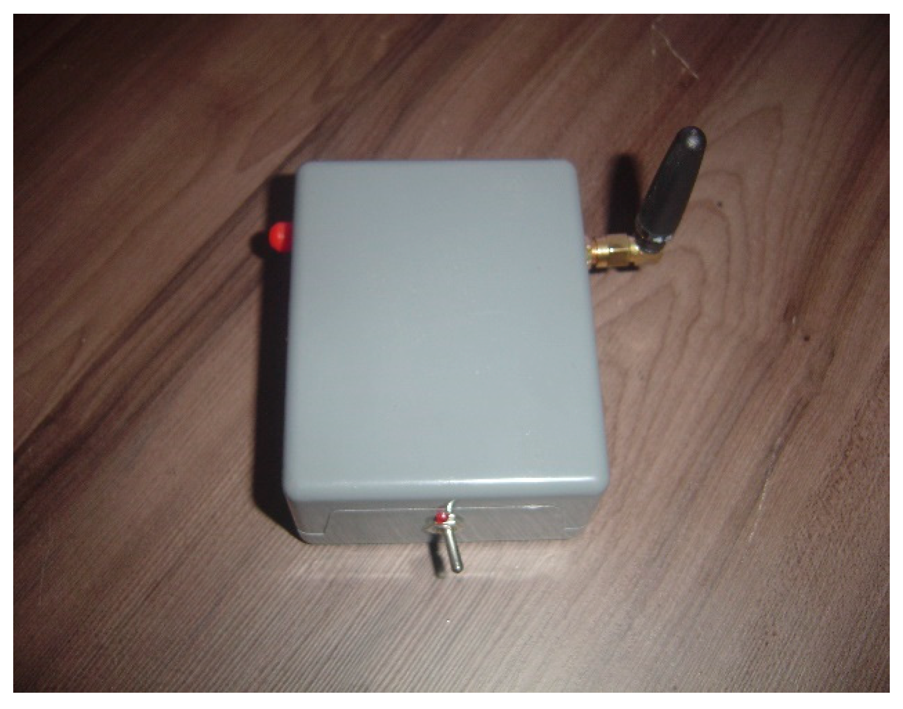Such a scheme of control can be seen in the flowchart of the Figure 2. The configuration of the tracker and the update of the firmware could be remotely done when necessary. 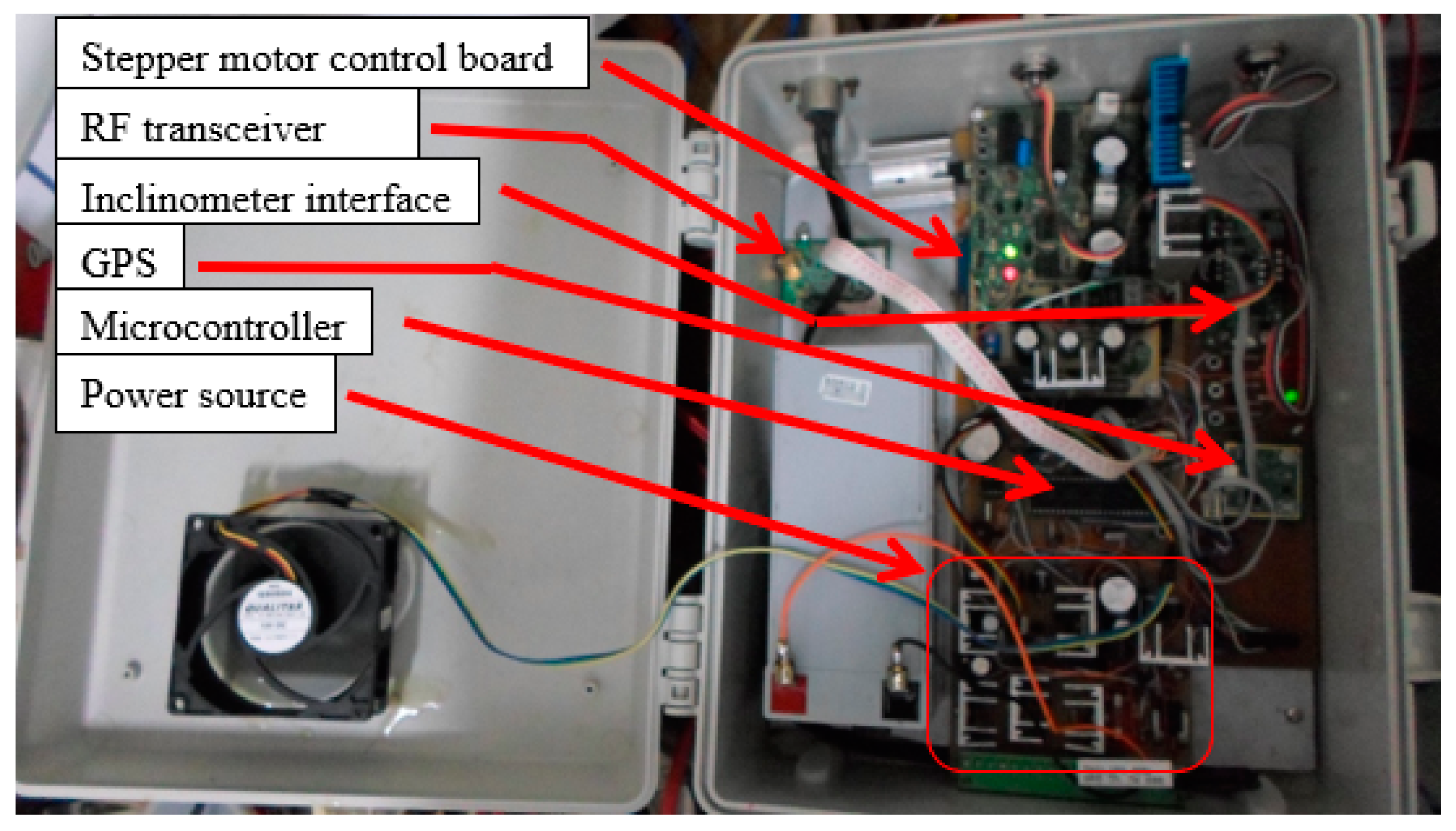As could be expected, a RF transceiver module counterpart, Figure 3, was connected to the desktop computer. In Figure 4, the electronics behind the flowchart can be observed. Finally, the supervisor software in the computer was written in the languages C++ and C#, while the firmware in the tracker was written in the assembler and C.

In order to calculate the solar position, the algorithm of Reda was selected due to its low value of uncertainties (±0.0003°) [13]. It has much more precision than necessary, indeed, regarding the goals of this work.

In the hardware of the solar tracker, by means of the GPS module, geographic data was measured, saved and sent to the supervisor, like the coordinates of the site, i.e., latitude and longitude (−8.054965°, −34.954948°), of the experiment located in Recife, state of Pernambuco, Brazil. After that, the software of the supervisor had built a look-up table of the positions, minute by minute, several days along in the approximate interval of 5:45 am to 5:30 pm. Finally, the look-up table was uploaded to the solar tracker and saved in the flash memory.

With the axis in polar mount direction, a stepper motor was coupled to a 1:20 reductor. By selecting a wave mode in the stepper motor control board configuration, a resolution of 0.09° per step was reached. Acting as a feedback signal by measuring the rotating angle, an inclinometer sensor (with accuracy of 0.1°) was placed attached at the side of the photovoltaic (PV) panel.

Designed to share the (same) window of one minute, there was 03 solar tracking strategies developed in software (firmware). As follows, each strategy by its time in a sequence, took the control of the hardware to move the panel according to its goal and save the data of the collected power:

• The strategy numbered 0 means a fixed polar mount in the horizontal place. So, at the end of the last strategy (or at the beginning), the panel moves back to this neutral position (null angle);
• When finished the time of the strategy above, the strategy numbered 1 takes its place and do the following: it retrieves the range of the whole day tracking angle of the (next) strategy 2 and divides it by 7, resulting in just seven segments of arc to track; then, it will select the position of the middle of the segment where the next strategy (numbered 2) will take place;
• Once finished the strategy number 1, the strategy numbered 2, which means a continuous tracking, also takes its place and simply adjusts the tracking angle, updating each minute through the look-up table previously saved in memory. Additionally, the position of the panel is set accordingly to the new angle.

In parallel, a solarimetric station, Figure 5, was responsible of measuring the direct, diffuse and global horizontal irradiance within the time window of each strategy, what has been recorded, second after second, by means of a datalogger model CR10-X. This way, with the collected energy measured and saved in the solar tracker memory for each strategy, it was possible to make comparisons with the irradiance measurements stored in the datalogger.

All the data produced was downloaded from the solar tracker flash memory and from the datalogger. Next, both were merged together for post processing in a PostgreSQL database with the aid of the download options in the supervisor software created for the desktop computer.

3. Results

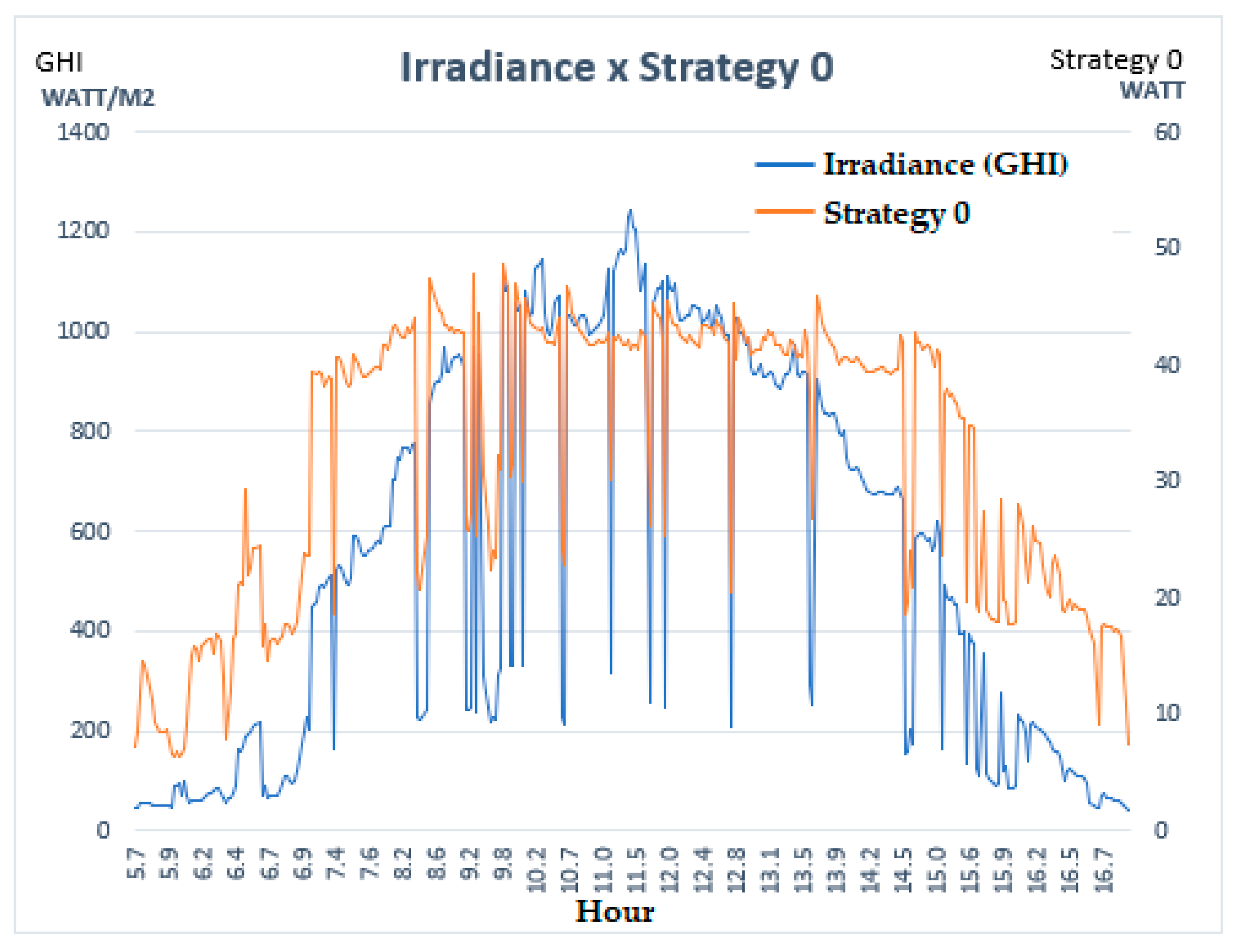
The period of data collection preceded the beginning of the rain season and it had an average rainfall of about 280 mm in the months of that experiment, marked by unstable and cloudy weather. It was reflected in the results, which can be easily seen in terms of the global horizontal irradiance (GHI) measurements. That parameter was used to filter the minutes shared by strategies to ensure that, in each minute, the standard deviation of the global horizontal irradiance was not greater than 10 W/m², being this amount the uncertainty of irradiance measurements of the solarimetric station. In other words, strategy samples were discarded when, within one-minute time intervals, the values of the standard deviation of irradiance are beyond the GHI uncertainty. That circumstance would represent changes due to atmospheric interferences as passage of clouds. Then, those samples were discarded when calculating the average power collected by the strategies in order to avoid a biased comparison among them.

The solar tracking accuracy along a day can be found by means of the deviation angle from the previously calculated solar positions, as is summarized in

Table 1. Summary of the deviations in strategies positioning.

Strategy/Metric	MAE (°)	RMSD (°)	MaxDev (°)
0	0.048	0.011	0.28
1	0.076	0.003	0.15
2	0.097	0.009	0.45

, regarded the measurements for each of the 03 strategies. The metrics RMSD, MAE and maximum absolute deviation are defined as follows:

$$RMSD= \sqrt{\frac{1}{N}{\Sigma }_{i=1}^N{\left(y_i- {\widehat{y}}_i\right)}^2}$$

(1)

$$MAE = \frac{1}{N}{\Sigma }_{i=1}^N\left(\left|y_i- {\widehat{y}}_i\right|\right)$$

(2)

$$MaxDev = Max\left(\left|y_i- {\widehat{y}}_i\right|\right)$$

(3)

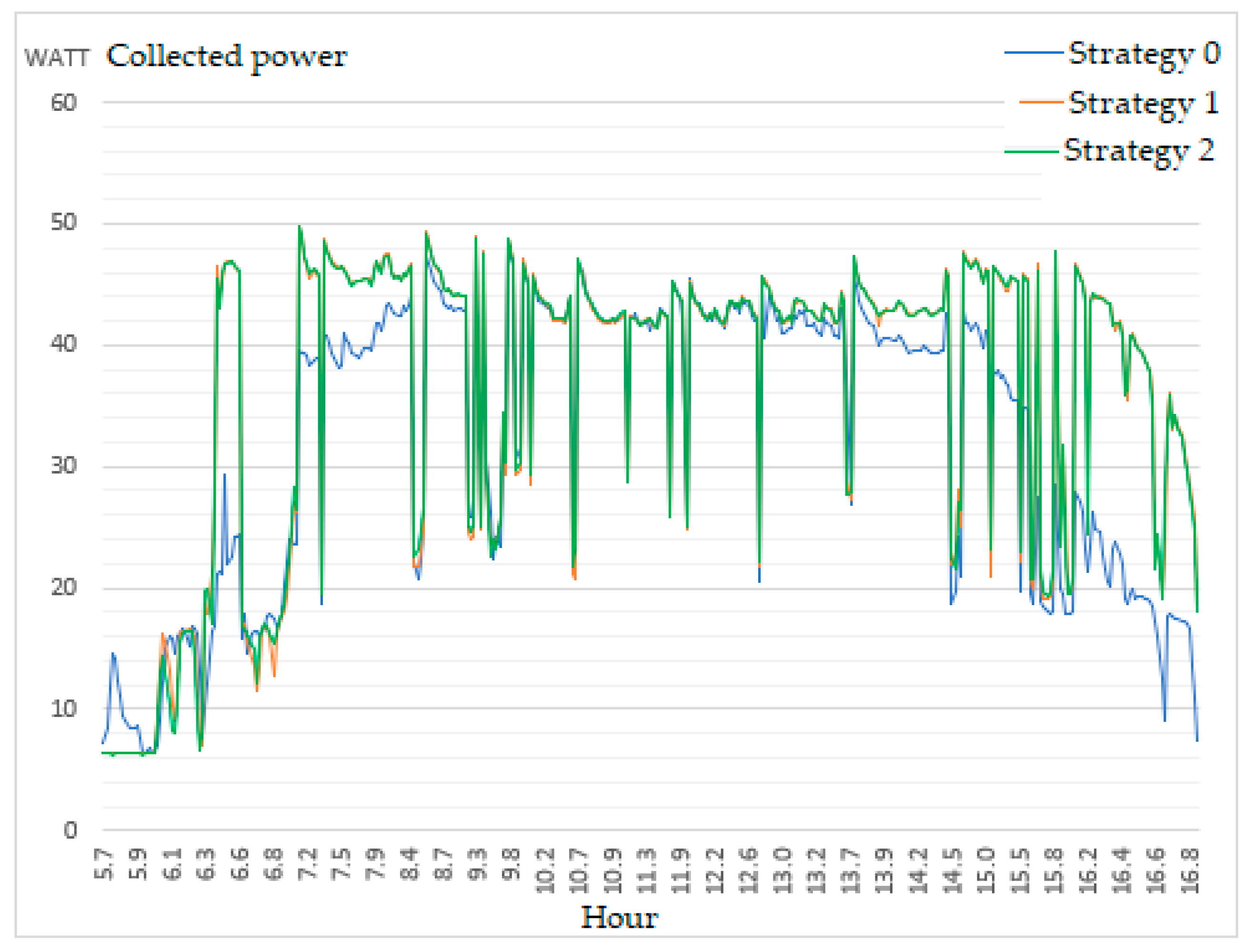
The graphics in Figure 6 and Figure 7 show the behavior of the global horizontal irradiance and the energy power received by the strategies along a partially cloudy day. It is noticed the absence of a reasonable difference between the received power regarding strategies 1 and 2. In a matter of fact, this happened in the same way during all the experiment periods. To explain the similarity in behavior about the strategies 1 and 2, it is useful to review solar geometry and the related concepts and definitions [19,20,21,22,23].

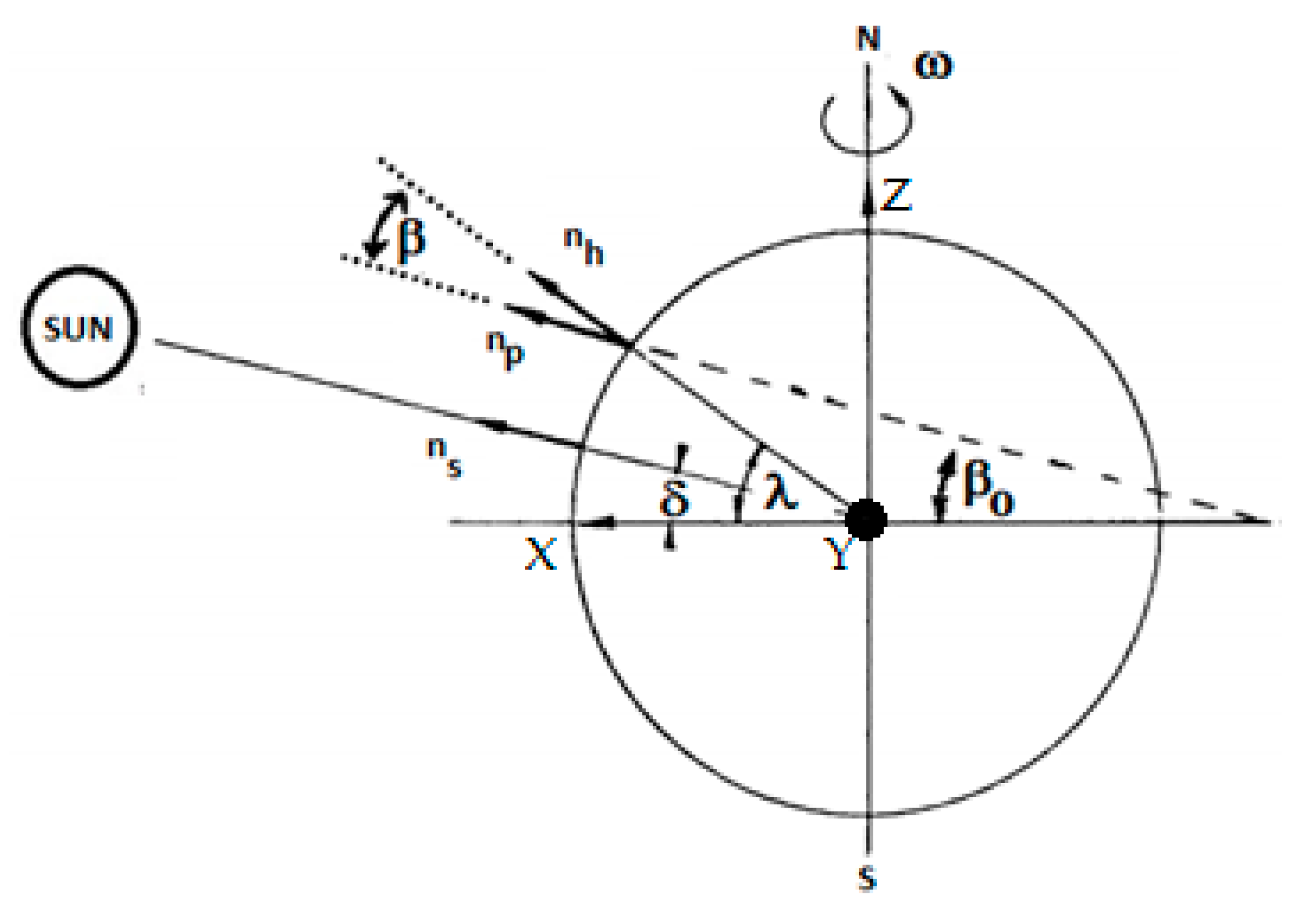
Starting from the Figure 8, it can be shown that the sun ray unity vector, $n_s$, can be expressed in the form:

$$n_s = (\cos \mathsf{\delta } \cos \mathsf{\omega } \cos {\beta }_0- \sin \mathsf{\delta } \sin {\beta }_0, - \cos \mathsf{\delta } \sin \mathsf{\omega }, \cos \mathsf{\delta } \cos \mathsf{\omega } \sin {\beta }_0 + \sin \mathsf{\delta } \cos {\beta }_0)$$

(4)

Given that ${{\psi }^{\prime }}_{NS}$ is the solar tracking angle considering a non-necessarily polar mount with a rotating axis in the north–south direction with the tracking error angle $\mathsf{\epsilon }$, it can be written as:

$${{\psi }^{\prime }}_{NS} = {\psi }_{NS} -\mathsf{\epsilon }$$

(5)

In which ${\psi }_{NS}$ is the tracking angle without error. Moreover, $n_p$, the unity vector normal to the panel, can be written as:

$$n_p = (\cos {{\psi }^{\prime }}_{NS}, -\sin {{\psi }^{\prime }}_{NS}, 0)$$

(6)

The dot product, $n_p$. $n_s$, is:

$$n_p . n_s= \cos {\theta }_{NS}= cos {{\psi }^{\prime }}_{NS}\left(\cos \mathsf{\delta } \sin \mathsf{\omega }/\tan {\psi }_{NS}\right)+ \sin {{\psi }^{\prime }}_{NS}\cos \mathsf{\delta } \sin \mathsf{\omega }$$

(7)

Which can be rearranged into a simpler expression:

$$\cos {\theta }_{NS}= \cos \mathsf{\delta } \cos \mathsf{\epsilon } \left(\frac{\sin \mathsf{\omega }}{\sin {\psi }_{NS}}\right)$$

(8)

So that:

• ${\theta }_{NS}$ is the angle formed by the sun ray and the normal to the PV panel. The NS subscript means the north–south direction of the axis;
• $\mathsf{\delta }$ is the declination of the sun;
• $\mathsf{\epsilon }$ is the tracking error;
• $\mathsf{\omega }$ is the hour angle;
• ${\psi }_{NS}$ is the tracking angle without error.

The variable $\cos {\theta }_{NS}$ has no dimension, but it will reflect the power loss (by square meter) when multiplied by the magnitude of the irradiance vector. For that reason, it is said to express a power loss in this text. The variable ${\psi }_{NS}$ can be calculated from the following expression:

$$\tan {\psi }_{NS}= \sin \omega /\left(\cos \omega \cos {\beta }_0-\tan \delta \sin {\beta }_0\right)$$

(9)

Additionally, the variable ${\beta }_0$ in the equation above can be stated as:

$${\beta }_0= \mathsf{\beta }- \mathsf{\lambda }$$

(10)

Still, $\mathsf{\lambda }, \mathsf{\beta } \mathrm{and} {\beta }_0$ are defined as:

• $\mathsf{\lambda }$ is the latitude of the site;
• $\mathsf{\beta }$ is the tilt (of the axis) from horizontal plane;
• ${\beta }_0$ is the tilt (of the axis) from equatorial plane.

The factor $\left(\frac{\sin \mathsf{\omega }}{\sin {\psi }_{NS}}\right)$ in Equation (8) can be interpreted as the instantaneous gain (or loss) of power associated to the axis tilt from the equatorial plane, ${\beta }_0$. That angle could be modified from a null value (the polar mount case) into another value in order, for instance, to increase the collected energy regarding the period of a specific season. In the case of a dual axis tracker, ${\beta }_0$ could be properly (and continuously) modified so that it would compensate the power loss due to the declination ($\cos \mathsf{\delta }$) in such a way to get $\cos {\theta }_{NS}=\cos \mathsf{\epsilon }$.

In the particular case of this work, a polar mount design, ${\beta }_0$ =0. As a consequence:

$$\tan {\psi }_{NS}= \tan \omega$$

(11)

This way, Equation (8) can be simplified into the following expression:

$$\cos {\theta }_{NS}= \cos \mathsf{\delta } \cos \mathsf{\epsilon }$$

(12)

Back to the comparison between strategies 1 and 2, as the panel is set in the middle of the arc in strategy 1, the power loss in the worst case due to the tracking error is about 2%, regarding an arc of 24° for each one of the seven positions of a total of 168°. However, that loss is better characterized by analyzing the average loss along the arc. Then, if the variation of the declination during each one of the seven arcs is neglect, the value on average of $\cos {\theta }_{NS}$ can be calculated as:

$$<\cos {\theta }_{NS}> = \cos \mathsf{\delta }<\cos \mathsf{\epsilon }>$$

(13)

After calculating the mean value of $\cos \mathsf{\epsilon }$, ε in the range of [0; ${\mathsf{\epsilon }}_m$], Equation (13) can be rewritten as:

$$<\cos {\theta }_{NS}> = \cos \mathsf{\delta }(\sin {\mathsf{\epsilon }}_m)/{\mathsf{\epsilon }}_m$$

(14)

Note that ${\mathsf{\epsilon }}_m$ is the maximum tracking error inside the arc. Let, in the case of strategy 2:

$$<\cos {{\theta }^{\prime }}_{NS}> = \cos \mathsf{\delta }(\sin {{\mathsf{\epsilon }}^{\prime }}_m)/{{\mathsf{\epsilon }}^{\prime }}_m$$

(15)

Now, once that $(\sin {{\mathsf{\epsilon }}^{\prime }}_m)/{{\mathsf{\epsilon }}^{\prime }}_m$ ≈ 1 in the strategy 2, then:

$$\frac{<\cos {{\theta }^{\prime }}_{NS}>- <\cos {\theta }_{NS}>}{<\cos {{\theta }^{\prime }}_{NS}>} \approx 1-(\sin {\mathsf{\epsilon }}_m)/{\mathsf{\epsilon }}_m$$

(16)

Then, the relative (average) loss of power of strategy 1 compared with 2 can be evaluated by Equation (16) above. It is opportune to observe that it could be understood as a comparison on a daily basis in each segment of arc of the strategy 1, given that the declination $\mathsf{\delta }$ is the same for both strategies. This geometric loss due to the seven positions can be calculated by taking into account that the maximum tracking error, ${\mathsf{\epsilon }}_m$, was about 12°. This represents a loss of, approximately, 0.73%, which explains the fact that no significant difference had been observed between strategies 1 and 2. Indeed, 0.73% in loss would be equivalent to a constant tracking error of 6.92°, almost half of 12°. It is also worth noting that seven positions meant a movement each 1 h and 36 min.

If, instead, the discrete tracking intervals had five or three positions, the relative power losses would be, respectively, 1.46% and 4.1%. By the other hand, choosing to increase the number of intervals to 9, 11 or 21, those associated losses would be 0.44%, 0.29% and 0.08%, respectively. This last option would mean a movement each 32 min.

On an annual basis, the left term in Equation (17) can be calculated as a function of the variation of declination $\mathsf{\delta }$ along the year. It means the annual average value of the power loss of the strategy 1 in comparison with a well tracked system. Indeed, it will have the dimension of power (by square meter) only after being multiplied by irradiance as commented before.

$$<(< \cos {{\theta }^{\prime }}_{NS}>- <\cos {\theta }_{NS}>)> = <\cos \mathsf{\delta }>(1-(\sin {\mathsf{\epsilon }}_m)/{\mathsf{\epsilon }}_m)$$

(17)

Equation (19) turns into the following expression, knowing that $\mathsf{\delta }$ is in the range of [0, ${\mathsf{\delta }}_m]$:

$$<(< \cos {{\theta }^{\prime }}_{NS}>- <\cos {\theta }_{NS}>)>=\left((\sin {\mathsf{\delta }}_m)/{\mathsf{\delta }}_m)\right)(1-(\sin {\mathsf{\epsilon }}_m)/{\mathsf{\epsilon }}_m)$$

(18)

As ${\mathsf{\delta }}_m\approx {23.45}^{°}$, $<\cos \mathsf{\delta }> =0.972$, so that Equation (18) can be rewritten as:

$$<(< \cos {{\theta }^{\prime }}_{NS}>- <\cos {\theta }_{NS}>)> \approx 97.2\%(1-(\sin {\mathsf{\epsilon }}_m)/{\mathsf{\epsilon }}_m)$$

(19)

During the calculations of power losses, an important assumption was done about the extraterrestrial irradiance being a constant value. If the variation of the irradiance along the year is regarded, it must be included when calculating the annual average losses, which can be done numerically. In time, it is prudent to note that the past calculations were based solely in geometric argumentation and other kinds of losses were not considered in a general way. At this point, it is useful to introduce a metric used to evaluate the cost effectiveness of the analyzed PV installations of solar plants, called LCOE (USD cents/kWh) and known as the levelized cost of energy. According to Lee [24], the LCOE takes into account several input parameters, like construction costs, operations and maintenance costs, the lifespan of the power plant, power generation technology, energy efficiency, system degradation rates, inflation interest rates and corporate taxes. This can be defined in a simple and basic way as:

$$LCOE=\frac{installation cost+financing cost+fuel cost+maintenance cost}{MWh produced over service life}$$

(20)

Once that there is not a solar plant with the n-positions (with a polar mount geometry) based on the solar tracker proposed in the present work, some input parameters can not be found in order to compare with other systems. However, the simplicity associated with a few positions along the way is supposed to be economically attractive as it can reduce the operation and maintenance costs in spite of the loss of 0.7% (or less for more than 7 positions a day) in energy harnessing when compared to a continuous single axis tracker in a similar geometry mount. If a solar tracker polar mounted that eventually updates its position on each deviation of 4°, which means an update each 16 min, have adopted the proposed solution with seven positions to cover an arc of 130°, it would save 25 movements a day, 750 movements a month and 9125 movements a year. Tracker systems that update their positions in a higher rate than one movement each 16 min would save movements even more.

4. Discussion and Conclusions

A review of the papers show that although all the experiments and models with a single-axis solar tracker did not have the same energy efficiency as a dual-axis system, that difference is becoming lower through the new approaches. At the same time, the research has advanced to get better results in simpler structures, which can be seen in an increasing number of solar trackers based on discrete solar tracker positions. This scenario is usually accompanied with a decrease in the costs. The investigation of the tradeoff between efficiency and simplicity was the main idea behind the research done in the present work where theory and the construction of a solar multitracker were combined altogether.

The purpose implemented along this work used seven tracking positions compared to continuous tracking, both sharing a 1-min time window, for a single axis solar tracker in a polar mount. The output of the strategies and the equations of the model developed here provided ways to evaluate theoretically the energy collected in the case of n-position single-axis solar tracking. By dividing an (tracking) arc of 168° in only seven tracking positions, it was not observed in measurements a clear contrast between the collected energy with respect to the discrete, seven positions and the continuous tracking strategy, in spite of having a small tracking error throughout all updates in the east–west rotation movements. This was confirmed by the study of the efficiency in relation to continuous tracking, revealing a theoretical loss value of about 0.73% in the 7-position strategy, which cannot be an easily measurable face to the uncertainties, especially in a partially cloudy day when such a difference can be smaller. However, if needed, it is possible to reduce the loss to as much as 0.08%, in the case of 21 positions a day, which requires movement every 32 min for a total arc of 168°. If the simplicity of a tracker is a mandatory aspect, with as few as three positions, the loss would be 4.1%. The losses of 0.08%, 0.73% and 4.1% were calculated as the daily average. According to Equation (19), to have an annual basis in average, the daily losses should be multiplied by 97.2%, the maximum limit for a fixed single axis in a polar mount solar tracker. Then, for instance, the seven tracking positions would receive 96.5% of the amount that the ideal dual-axis solar tracker would collect. Additionally, with three positions, it would yield 93.2% a year on average.

In addition to the polar mount, Equation (8), which takes into account the tracking error, allows the numerical simulation of continuous and discrete tracking systems when the tracking axis is in the north–south direction, but not necessarily in a polar configuration. An article seen before reported four yearly adjusts in the tilt of the north–south axis to enhance the collection of energy. In other case, the determination of optimum performance of a single-axis on an ISNA geometry as a function of the tilt angle along the seasons was the object of the study in the paper of Ghosh [25], which could also be simulated in Equation (8) by including the discrete positions along the day.

With the support of computational simulations, the work of Zhu managed to get, in a design called the TR-axis, 96.4% of the energy that would be collected with a dual-axis tracker [11]. However, the simulation returned 95.79% for a polar assembly, lower than that theoretical value presented here (97.2%) when a continuous single axis solar tracker in a polar mount was regarded. It is worth mentioning that the present study did not sum up the contribution of the diffuse irradiance as in the article cited. Through the use of mathematical simulations and also including the parcel of diffuse radiation, the work of Li found that the optimal angle within an ISNA (single axis) geometry for collecting solar energy was obtained with a 3° deviation from the polar mount, yielding about 97–98% of dual-axis solar tracking [10]. The work of Gosh based on an ISNA configuration, north–south seasonal adjustments in the axis and diffuse irradiance computed managed to have collected 98.22% of the energy in a dual-axis [25].

As a next step in this work, it is intended to study the gain in the collected energy with respect to an ISNA mount type, in seasons taking into account the diffuse irradiance. Another goal is the investigation of the discrete solar tracking in such cases, beyond the polar assembly. Finally, in spite of having no commercial solar plant using the present n-position single axis solar tracker proposed and, by consequence, having no economic data to be evaluated as prices, costs and power production rates of such implementation, it is believed that the simplicity offered along this study could compensate and surpass the traditional polar mount single axis tracker in the economic point of view.