Methodology for Assessing the Stability of Drilling Rigs Based on Analytical Tests

Abstract

Underground mining machines, such as wheel-tyre drilling rigs, are articulated and equipped with booms that project far beyond the undercarriage. Such a structure makes these machines prone to losing stability. Hence, it is necessary to analyse the distribution of masses and geometry as well as their broadly understood stability during the entire design process, taking into account many factors resulting from the manner and conditions of their operation. However, there are no appropriate computational models that would enable analytical tests to be carried out for machines with this kind of construction. This article is concerned with the author’s computational model, which allows the stability of single- and twin-boom drilling rigs to be quickly assessed. The model makes it possible to perform analyses without having to solve differential equations that are present in dynamic models or using specialist software based on CAD and CAE tools. The developed model allows determination of the pressure of wheels and jacks as a function of many important parameters and variables. Additionally, the distances of the centre of gravity from the tipping edge are calculated. The developed computational model was verified by comparing the obtained results with the results of the full dynamic model, the results of model tests carried out in the CAD/CAE program, and the results of empirical tests of wheel and jack pressures on the ground for the selected drilling rig. The model was subjected to verification and validation, which proved that it was fully correct and useful. The model was used to prepare a practical and user-friendly calculation sheet. Apart from the numerical values, the calculation sheet contains a graphical representation of the machine, the location of the centre of gravity, the tipping edges, as well as graphs of the wheel and jack pressures. Next, analytical tests of the stability of the selected drilling rig were carried out. The obtained calculation results are consistent with the results of empirical research. The computational model and the spreadsheet provide handy tools used during the design process by one of the Polish company’s producing drilling rigs.

1. Introduction

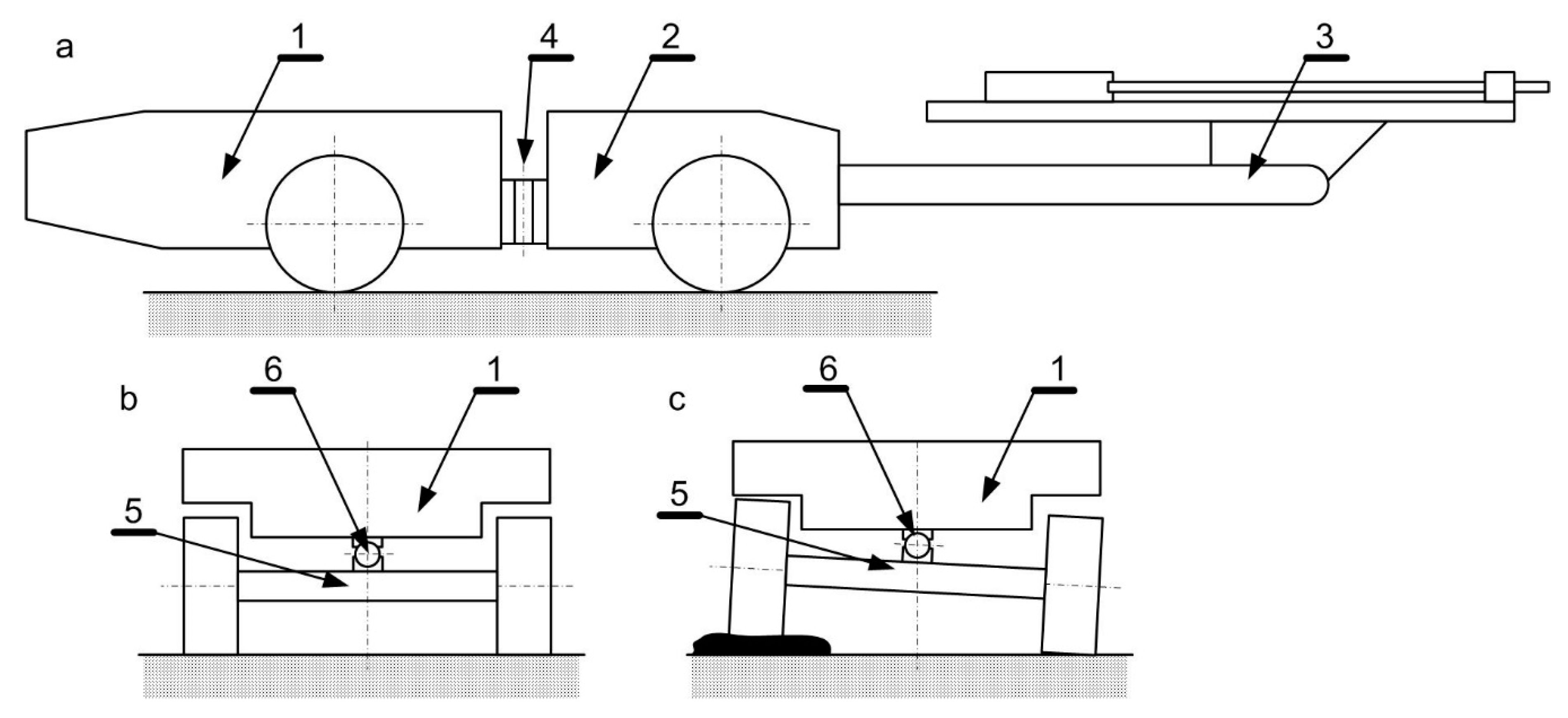
Self-propelled mining machines, such as wheel drilling rigs, have an articulated structure, which due to the use of long booms, working conditions, and requirements regarding the turning radii is prone to losing stability. Figure 1 shows a diagram of a single-boom drilling rig. In Figure 1a, the side view is presented, whereas in Figure 2b,c, the rear view. The drilling rig consists of a rear body 1 seated on an oscillation axle 5 (Figure 1b). Between the rear body 1 and the oscillation axle 5, there is a joint 6 with a horizontal axis. The articulated oscillation axle enables driving on an uneven surface (Figure 1c). The rear body 1 is connected to the platform 2 by means of a joint with a vertical axis 4. The articulated connection of the rear body and the platform together with appropriate hydraulic cylinders is responsible for the turning of the machine. One or two booms 3 are attached to the platform. More booms, three or, less frequently, four, are used only in the case of very big rigs.

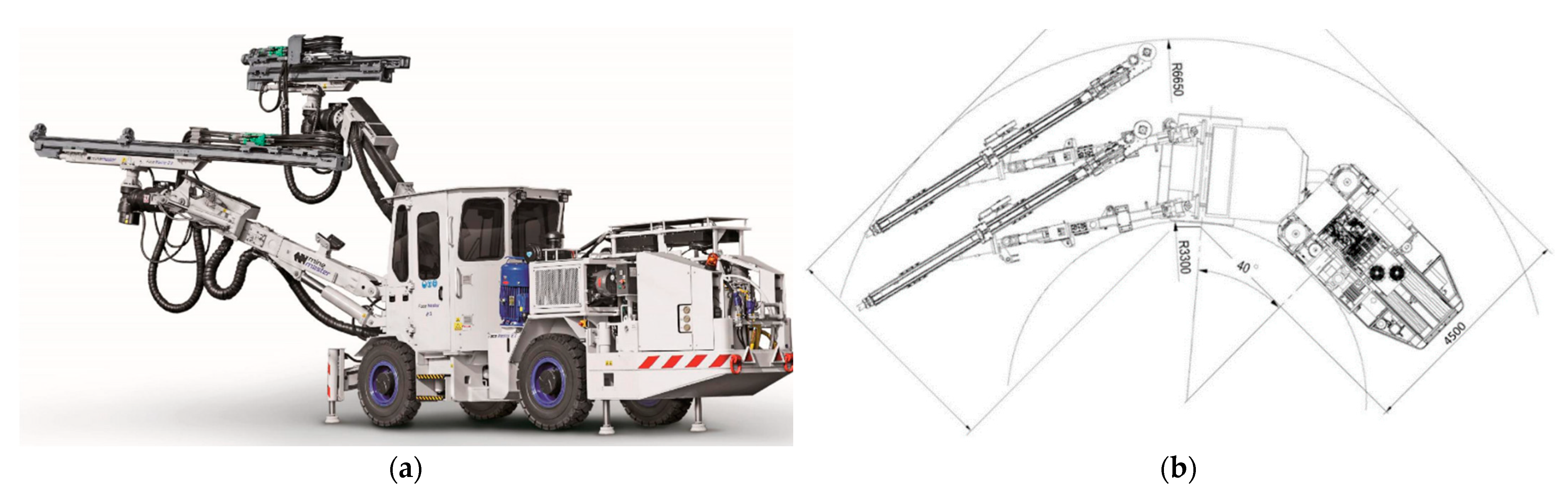
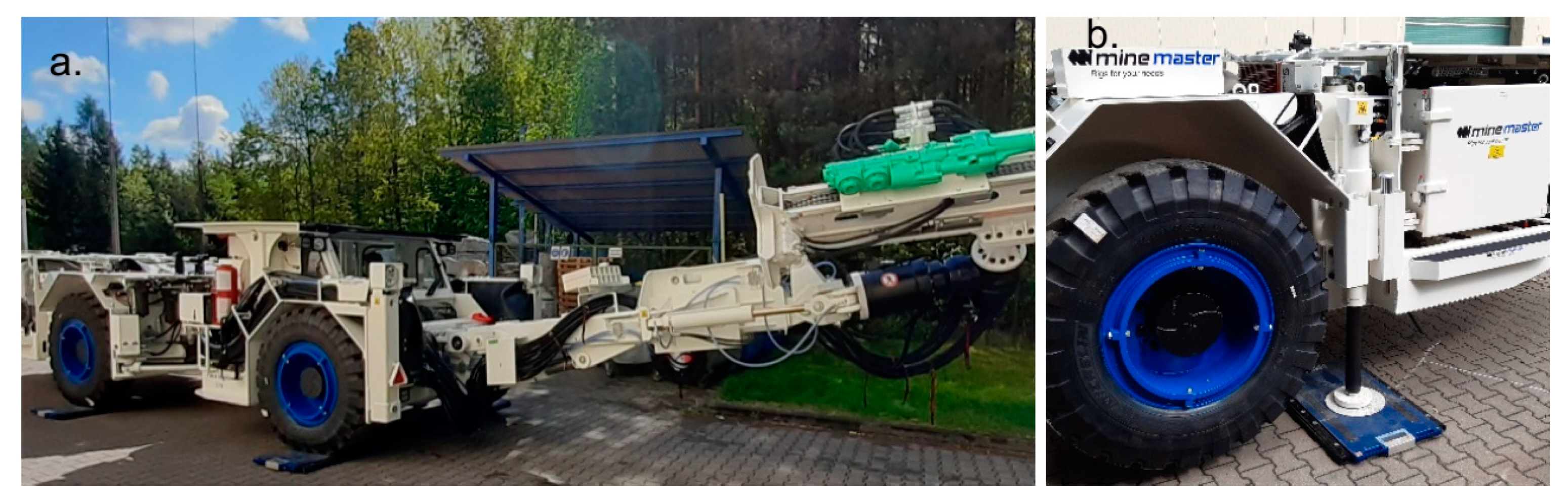
Figure 2a shows a Face Master 2,3 drilling rig produced by Mine Master [1], whereas Figure 2b presents its arrangement when driving in excavations. The total length of drilling rigs reaches ca 11–14 m, the width is approximately 1.8–2.5 m, and the height is 1.5–3.0 m. The total weight ranges from 13 tons to even 30 tons. The wheelbase is approximately 3–4 m, and the booms extend more than 6 m beyond the front axle. When taking bends, the machine is turned by an angle of up to 40° and, additionally, in narrow workings, the booms swing sideways, sometimes by more than 10°. During operation, the booms extend far beyond the outline of the machine chassis and allow holes to be made in underground workings with a cross-section of several dozen square meters. Typically, the booms tilt 45° upwards, 25° downward, and 35° to 55° sideways. In addition, during operation, the telescopic booms extend by approximately 1.5 m. Therefore, during both manoeuvring and operation, these machines tend to lose stability. The stability of self-propelled mining machines is a key issue, especially in the process of developing new solutions that meet the high demands of users and difficult working conditions.

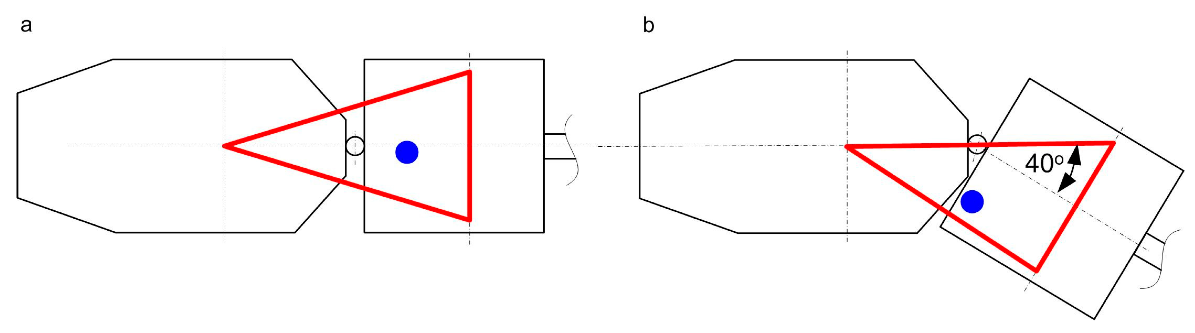
Such a machine is stable when its centre of gravity is inside the triangle defined by the centres of the front wheels and the centre of the oscillation axle (Figure 3a). The lines connecting these points are called the edges of tipping. During cornering manoeuvres, the centre of the oscillation axle moves and, at the same time, the resultant centre of gravity of the machine shifts strongly towards the tipping edge, thus reducing the stability of the machine (Figure 3b). The situation is worsened by inclined excavations and boom swing. An incorrectly designed machine can be prone to losing its stability.

Currently, modern methods and tools are used to design and test working machines, including mining machinery [2,3,4,5,6]. Computer-aided design (CAD) and computer-aided engineering (CAE) programs have been applied, and theoretical models and research stands have been developed [7,8,9,10]. Ergonomics and occupational safety are gaining increasing importance [11]. Increasingly more new solutions of machines and machine elements are being developed on an ongoing basis [12,13,14,15]. From the very beginning of the drilling rig design process, it is necessary to analyse the values of the mass, geometry, and the location of the centres of gravity of key components while simultaneously assessing the stability of the machine. Stability is influenced by the longitudinal and transverse slope of the excavation, the turning of the machine body, and the rotation of booms. In addition, sudden braking and driving on uneven terrain should be taken into account. Currently, theoretical models enabling quick analyses and assessment of the stability of such machines are not available. It is possible to perform simulation tests using CAD/CAE tools, for example, the Dynamic Simulation module in Autodesk Inventor Professional. However, such studies are time-consuming and require the. Development of appropriate models for each machine, which limits the possibility of conducting a comprehensive analysis for many variants of parameters. It is also possible to create a dynamic model, but it must be developed for each machine separately, and the results can be obtained after solving the differential equations.

Information on the stability of the machine can be obtained by conducting test runs and empirical tests on truck scales Practice shows that for this type of machine, the minimum pressure of one wheel on the ground above 1000 kg guarantees the stability of the machine. However, such measurements on the finished machine, for obvious reasons, cannot be performed at the design stage. Besides, at the time of test runs and empirical research, the possibility of making any changes is greatly reduced in practice, as it boils down to loading the machine with ballast in the form of steel sheets.

The stability of various types of working machines is a well-known problem, which has been extensively described in the literature. Generally speaking, the problem of rollover stability comes down to analysing the location of the machine’s centre of gravity in relation to the tipping edge [16]. In addition, especially in the case of cranes, the overturning and stabilizing moments as well as the tipping stability factor are calculated.

Machines that are typically prone to overturning, such as cranes, are frequently the subject of research and articles [17,18,19,20]. However, they are based on completely different design solutions, which usually work after levelling and when the machine is idle.

Solutions applied in articulated machines are closer to those found in the drilling rigs subjected to analysis. There are general theoretical models for the four-wheel chassis itself [21] or for vehicles with multiple axles [22]. An interesting articulated machine, but on a caterpillar chassis, has been presented in one of the articles. The authors showed a complex dynamic theoretical model and the results of analytical research [23].

Many studies concern agricultural machines, articulated machines, and ones with rigid frames. Due to machine operation on a terrain with longitudinal and transverse slopes, there is also a problem of stability. The authors present various static and dynamic models as well as the results of empirical research [24,25,26].

As regards articulated mining machines, there are a number of studies on load-haul-dump (LHD) loaders. In one of the articles, the problems of working machines’ rollover stability have been presented, with a special emphasis on the various solutions applied in LHD loaders [27]. The authors focused on the proprietary research stand, which enables empirical assessment of the stability and the verification of theoretical models. The stand allows simulation of the inclination of an articulated machine model while measuring the pressure of the wheels on the ground. In another article, the same authors conducted a comprehensive study of a loading machine stability and developed an appropriate theoretical model. As a result, they proposed changes positively influencing the stability of an articulated wheel loader [28].

Similarly, another team studied the stability of an articulated LHD loader in several subsequent articles [29,30,31]. Various dynamic models and several scale versions of the loader have been developed. The results provided by theoretical models were verified by the test results. Apart from typical situations, driving over obstacles of various shapes and sizes was also analysed. As regards the contact of wheels or jacks with the ground, there are numerous studies on the mechanical properties of rocks determined by various methods and under different conditions [32,33,34].

The above quoted studies are devoted to machines of a different design and contain descriptions of dynamic models, empirical research, or simulation tests. They also concern underground mining but are limited to much simpler machines, such as LHD loaders. Moreover, the aim of the works in question was to create a universal parametric computational model for assessing the stability of single- and double-boom drilling rigs. The model must enable calculations to be performed in a spreadsheet. The presented calculation methodology was developed due to the lack of available parametric theoretical models that would enable assessment of the stability of drilling rigs.

2. Methodology

The aim of the works in question was to create an accessible calculation sheet that would allow reliable results of calculating the stability of articulated single- and double-boom drilling rigs to be obtained. In the first stage, a physical model of the machine was developed based on the analysis of the drilling rigs’ documentation and information obtained from the project team. A number of assumptions were specified, taking into account the requirements and recommendations of the future user of the calculation sheet. Next, the physical model was saved as a mathematical model. A static computational model was created. The model was saved as a transparent spreadsheet in MathCad Prime Express. Then, the model was saved in the form of an accessible calculation sheet in Microsoft Excel. Entering complex calculation models and formulas in Excel is onerous. Moreover, it entails the risk of making simple errors because the pattern is written in one line, and frequently in many cells. Besides, Excel does not verify the compliance of the units or convert them. Therefore, the Mathcad spreadsheet was used to compare the obtained results. This approach made it possible to eliminate all errors when creating an Excel sheet.

The next stage involved verification and validation of the developed model on the basis of 3 machines: Face Master 2.3 single-boom, Face Master 2.3 double-boom, and Face Master 2.8 double-boom. For the purposes of verification, 3D models of drilling rigs were created in the Autodesk Inventor Professional environment. The 3D models allowed verification of the correctness of the formulas for global coordinates, coordinates of the centres of gravity of components and the entire machine, as well as the distances of the centre of gravity from the tipping edge.

Then, dynamic simulations were performed in Inventor, Dynamic Simulation and the values of the wheel pressure forces were determined, which were next compared to the results from the Excel spreadsheet. Various machine and boom settings were analysed.

In addition, the results from the Excel spreadsheet were compared with those from the report prepared for the dynamic model. The report was prepared by an independent research unit. For the purposes of this report, an external scientific unit used specialized a proprietary dynamic study developed for each machine. The comparison concerned selected configurations of machine parameters.

Validation of the model saved in the form of an Excel spreadsheet involved comparing the calculation results with the results of empirical research. The empirical tests, which were carried out by an external certified unit, consisted in measuring the pressures of wheels and jacks on the scales for each machine: straight, twisted, and for various positions of the booms.

In each case, the same data was adopted for each model in terms of the geometry of the rigs, masses, and positions of the centres of gravity, and variables, such as the turning angle or boom rotation angles. In this article, the results are shown on the example of the Mine Master Face Master 2.8 (FM 2.8) machine.

3. Theoretical Computational Model

In order to develop a physical and, next, a mathematical model, assumptions and guidelines, including appropriate acceptable simplifications, were defined. Then, formulas and equations were derived to calculate the location of the centre of gravity of the machine, its distance from the edge of tipping, as well as the pressure of wheels and jacks on the ground.

3.1. Assumptions for the Computational Model

Due to the need to develop an analytical model enabling a quick assessment of machine stability, a number of assumptions for such a methodology were specified in an Excel spreadsheet. First of all, the model must allow calculation of the pressure of wheels and jacks on the ground as well as the location of the centre of gravity and its distance from the tipping edge without necessarily having to solve differential equations. Based on the analysis of the construction of drilling rigs, it was assumed that the model would be developed for an articulated machine with an oscillation axle on a wheel-tyre chassis. The elasticity of wheels is simplified to a linear relationship in the model.

Single- and twin-boom solutions for moving in workings with a longitudinal slope of up to 20° and a transverse slope of up to 10° were designed. Dynamic forces acting on the machine due to braking and driving over a drop were taken into account. The centrifugal force was neglected as it contributes to the stability of these machines. The zero value of the centrifugal force, i.e., stopping the machine while turning, is the least favourable case, hence a model was created for this situation. Moreover, it was assumed that dynamic forces due to braking and driving on an uneven terrain take the form of static forces influencing the stability of the machine.

For each simplification, analyses and comparative calculations were carried out in order to determine their influence on the obtained results. The adopted assumptions and simplifications do not have a negative impact on the results. The elasticity of the wheels lowers the machine’s centre of gravity. The deflection of the wheels reached 20–50 mm. The lowered centre of gravity has a positive effect on the stability of the machine, especially in the case of an inclined excavation. The use of a linear relationship instead of a quadratic function has a slight influence on the results for this deflection range. The reduction of the longitudinal and transverse slope of the excavation results from the user’s requirements and the machine operating conditions. It allowed some components of the forces that had little impact on the calculation results to be ignored but allowed their significant simplification. From the point of view of stability, replacing the inertia forces with static forces is a favourable simplification. The model ignores the mass moments of inertia, hence the machine shows a greater margin of stability than the results from the calculations. The last assumption was disregarding the centrifugal force. The centrifugal force has a beneficial effect on the machine stability, so the least favourable case occurs when the car is stopped on a curve. Such a case was adopted in the model.

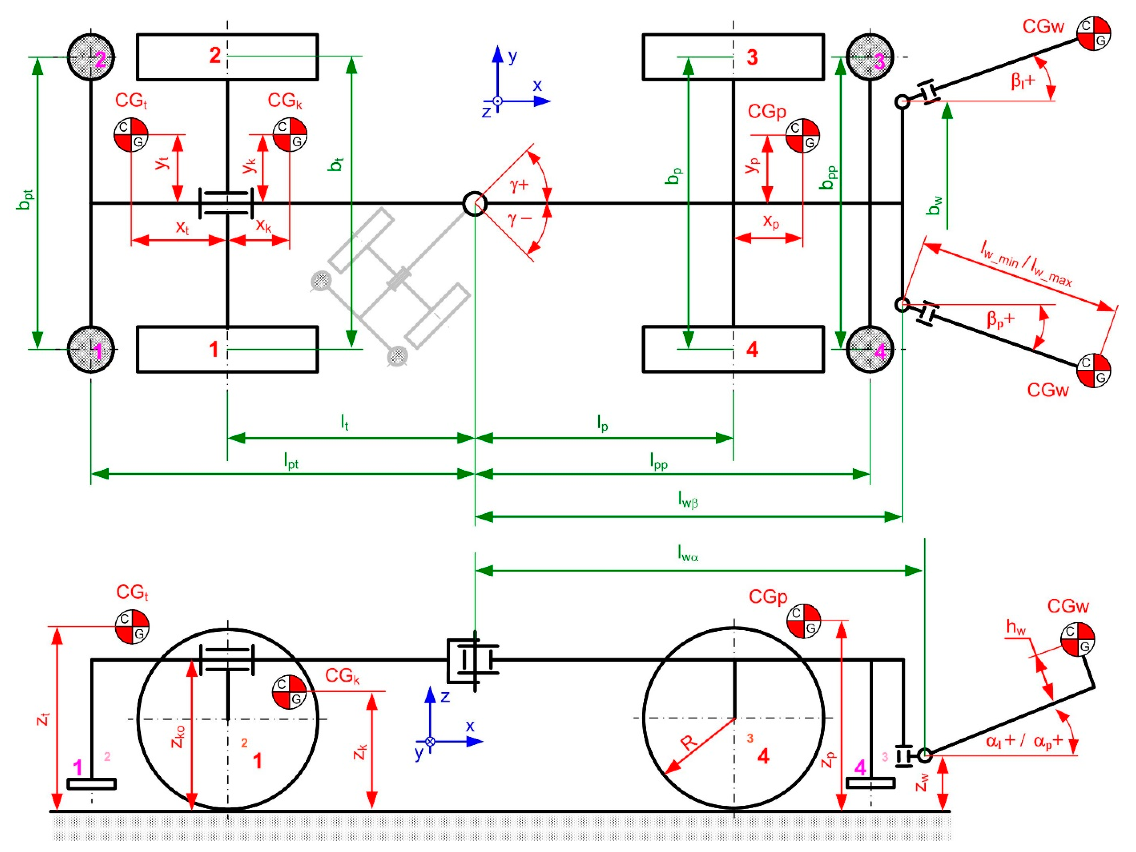
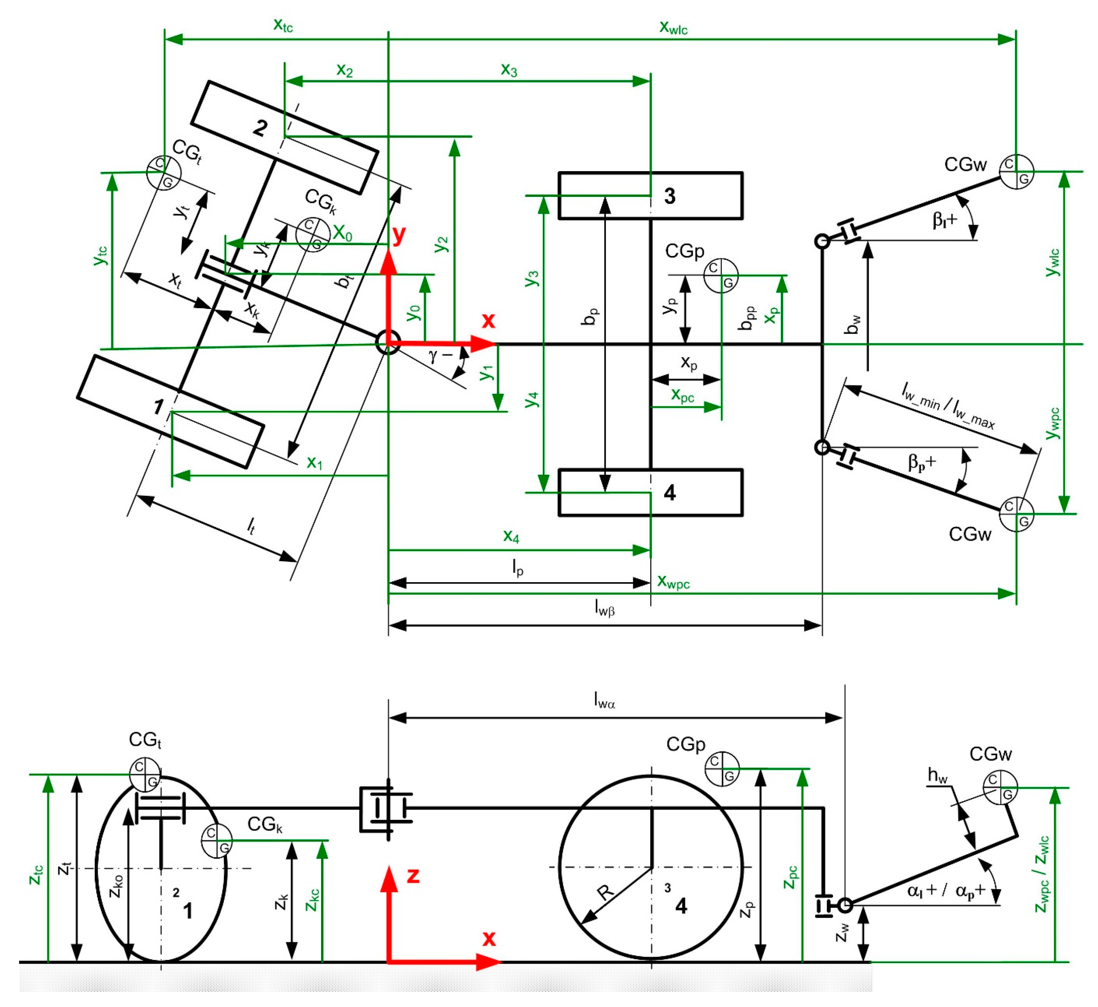
Determining the location of the centre of gravity of a drilling rig requires distributing its mass into individual components, which perform relative motion. In accordance with the assumptions, the rig was presented in terms of the masses and locations of the centres of gravity of: the rear body, the oscillation axle, the platform, and two booms. The most important geometrical parameters are the distances between the wheels and the machine’s joint and the quantities describing the position of the two pivot points of the boom for the horizontal and vertical axes. Additionally, the turning angle of the machine as well as the angle of boom rotation must be taken into consideration. The listed quantities are presented in the diagram shown in Figure 4.

3.2. Determination of Global Coordinates

The above-mentioned geometric parameters are described in a diagram in a way that facilitates their error-free and relatively easy determination. The positions of the centres of gravity as well as the positions of the centres of the wheels and oscillation axle change depending on the chassis turning angle and boom rotation angles. For the purpose of analysing the entire rig, it is necessary to assign the values of the x, y, and z coordinates in the global system. Based on the design of the rig and the defined assumptions, the centre of gravity was linked as follows:

• The centre of the coordinate system in the top view is in the joint;
• The x and y axes are identical to the x and y axes of the platform;
• The floor plane, defined by the contact of the tyres with the floor, is the xy plane;
• The z axis is perpendicular to the floor and, therefore, it is in line with the vertical axis of the machine.

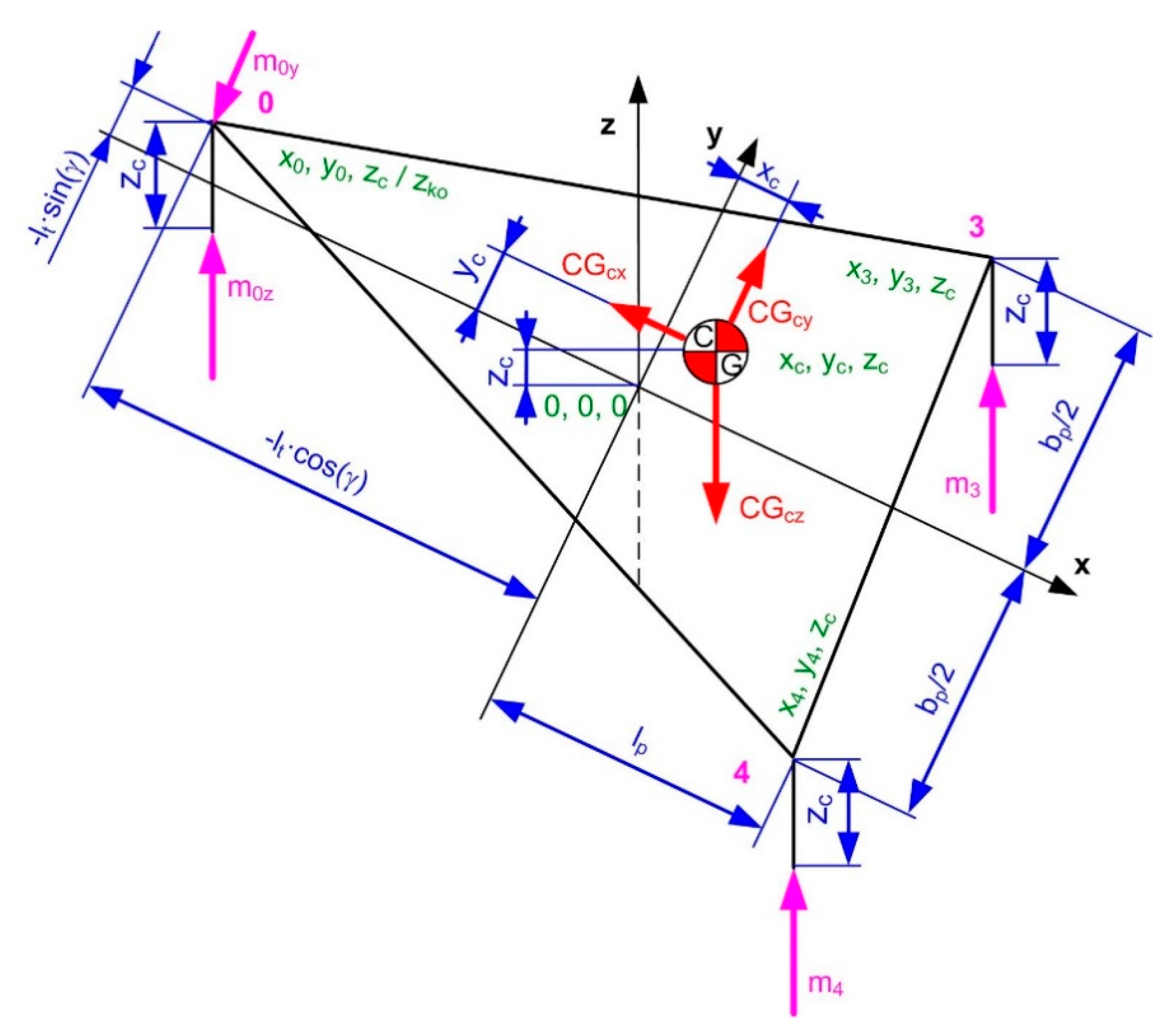
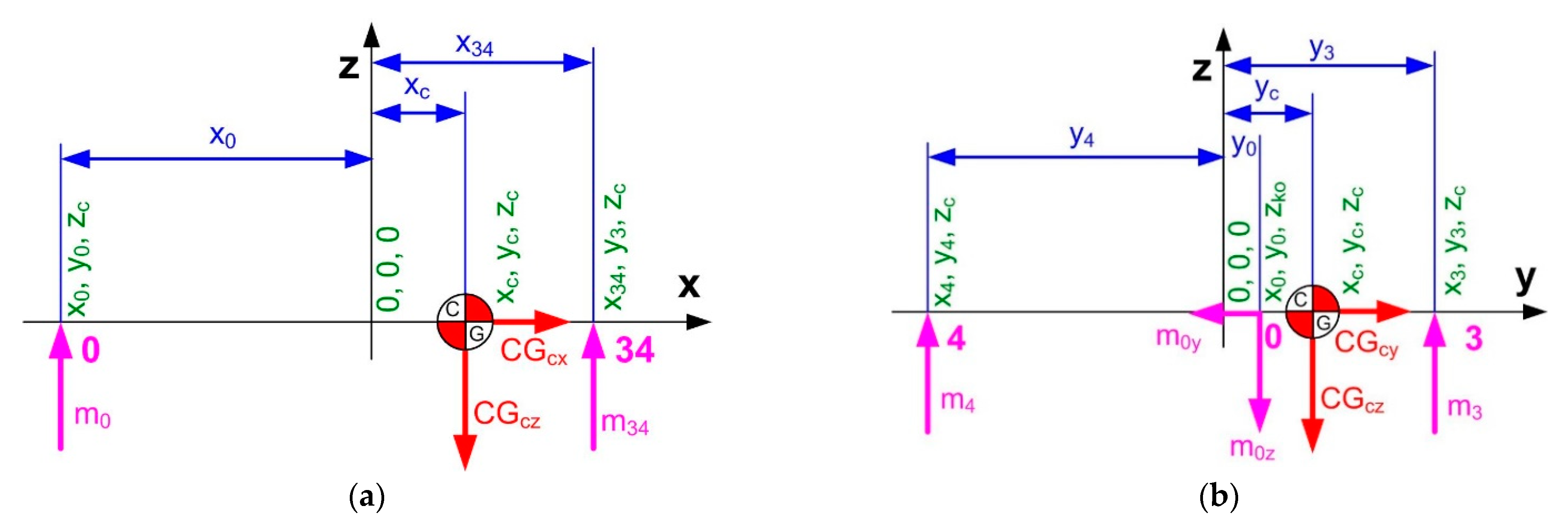
Therefore, appropriate formulas for x, y, and z in the global system were derived for each coordinate related to the centre of gravity and for the position of the booms, the position of each wheel, and the position of the oscillation axle centre. When deriving the formulas, the previously adopted subscripts were used, with the additional “c” denotation. In addition to the previously adopted subscripts, the “x” wheel numbers from 1 to 4 (without “c”) and the “xo” coordinate for the oscillation axle were also assigned. Several examples of coordinates are shown in Figure 5.

The below formulas derived for the analysed case enable determination of the global coordinates. Standard transformations as well as formulas for vector transformations and rotations were used in the process.

Coordinates of the rear body’s centre of gravity:

$$x_{tc}=-\left(l_t+x_t\right)\cdot \cos \left(\gamma \right)-y_t\cdot \sin \left(\gamma \right)$$

(1)

$$y_{tc}=-\left(l_t+x_t\right)\cdot \sin \left(\gamma \right)+y_t\cdot \cos \left(\gamma \right)$$

(2)

$$z_{tc}=z_t$$

(3)

Coordinates of the oscillation axle’s centre of gravity:

$$x_{kc}=-\left(l_t+x_k\right)\cdot \cos \left(\gamma \right)-y_k\cdot \sin \left(\gamma \right)$$

(4)

$$y_{kc}=-\left(l_t+x_k\right)\cdot \sin \left(\gamma \right)+y_k\cdot \cos \left(\gamma \right)$$

(5)

$$z_{kc}=z_k$$

(6)

Coordinates of the platform’s centre of gravity:

$$x_{pc}=l_p+x_p$$

(7)

$$y_{pc}=y_p$$

(8)

$$z_{pc}=z_p$$

(9)

Coordinates of the right boom’s centre of gravity:

$$\begin{array}{ll}\hfill x_{wpc}=l_{w\beta }+\left(l_{w\alpha }-l_{w\beta }\right)\cdot \cos \left({\beta }_{wp}\right)& +l_{ww}\cdot \cos \left({\alpha }_{wp}\right)\cdot \cos \left({\beta }_{wp}\right)\hfill \\ & -h_w\cdot \sin \left({\alpha }_{wp}\right)\cdot \cos \left({\beta }_{wp}\right)\hfill \end{array}$$

(10)

$$\begin{array}{ll}\hfill y_{wpc}=\frac{-b_w}{2}-\left(l_{w\alpha }-l_{w\beta }\right)\cdot \sin \left({\beta }_{wp}\right)& -l_{ww}\cdot \cos \left({\alpha }_{wp}\right)\cdot \sin \left({\beta }_{wp}\right)\hfill \\ & +h_w\cdot \sin \left({\alpha }_{wp}\right)\cdot \sin \left({\beta }_{wp}\right)\hfill \end{array}$$

(11)

$$z_{wpc}=z_w+l_{ww}\cdot \sin \left({\alpha }_{wp}\right)+h_w\cdot \cos \left({\alpha }_{wp}\right)$$

(12)

Coordinates of the left boom’s centre of gravity:

$$\begin{array}{ll}\hfill x_{wlc}=l_{w\beta }+\left(l_{w\alpha }-l_{w\beta }\right)\cdot \cos \left({\beta }_{wl}\right)& +l_{ww}\cdot \cos \left({\alpha }_{wl}\right)\cdot \cos \left({\beta }_{wl}\right)\hfill \\ & -h_w\cdot \sin \left({\alpha }_{wl}\right)\cdot \cos \left({\beta }_{wl}\right)\hfill \end{array}$$

(13)

$$\begin{array}{ll}\hfill y_{wlc}=\frac{-b_w}{2}-\left(l_{w\alpha }-l_{w\beta }\right)\cdot \sin \left({\beta }_{wl}\right)& -l_{ww}\cdot \cos \left({\alpha }_{wl}\right)\cdot \sin \left({\beta }_{wl}\right)\hfill \\ & +h_w\cdot \sin \left({\alpha }_{wl}\right)\cdot \sin \left({\beta }_{wl}\right)\hfill \end{array}$$

(14)

$$z_{wlc}=z_w+l_{ww}\cdot \sin \left({\alpha }_{wl}\right)+h_w\cdot \cos \left({\alpha }_{wl}\right)$$

(15)

Coordinates of the location of the contact of the wheel marked with number 1:

$$x_1=-l_t\cdot \cos \left(\gamma \right)+\frac{b_t}{2}\cdot \sin \left(\gamma \right)$$

(16)

$$y_1=-l_t\cdot \sin \left(\gamma \right)-\frac{b_t}{2}\cdot \cos \left(\gamma \right)$$

(17)

Coordinates of the location of the contact of the wheel marked with number 2:

$$x_2=-l_t\cdot \cos \left(\gamma \right)-\frac{b_t}{2}\cdot \sin \left(\gamma \right)$$

(18)

$$y_2=-l_t\cdot \sin \left(\gamma \right)+\frac{b_t}{2}\cdot \cos \left(\gamma \right)$$

(19)

Coordinates of the contact of the wheel marked with number 3:

$$x_3=l_p$$

(20)

$$y_3=\frac{b_p}{2}$$

(21)

Coordinates of the location of the contact of the wheel marked with number 4:

$$x_4=l_p$$

(22)

$$y_4=-\frac{b_p}{2}$$

(23)

Coordinates of the location of the oscillation axle (marked with number “0”):

$$x_0=-l_t\cdot \cos \left(\gamma \right)$$

(24)

$$y_0=-l_t\cdot \sin \left(\gamma \right)$$

(25)

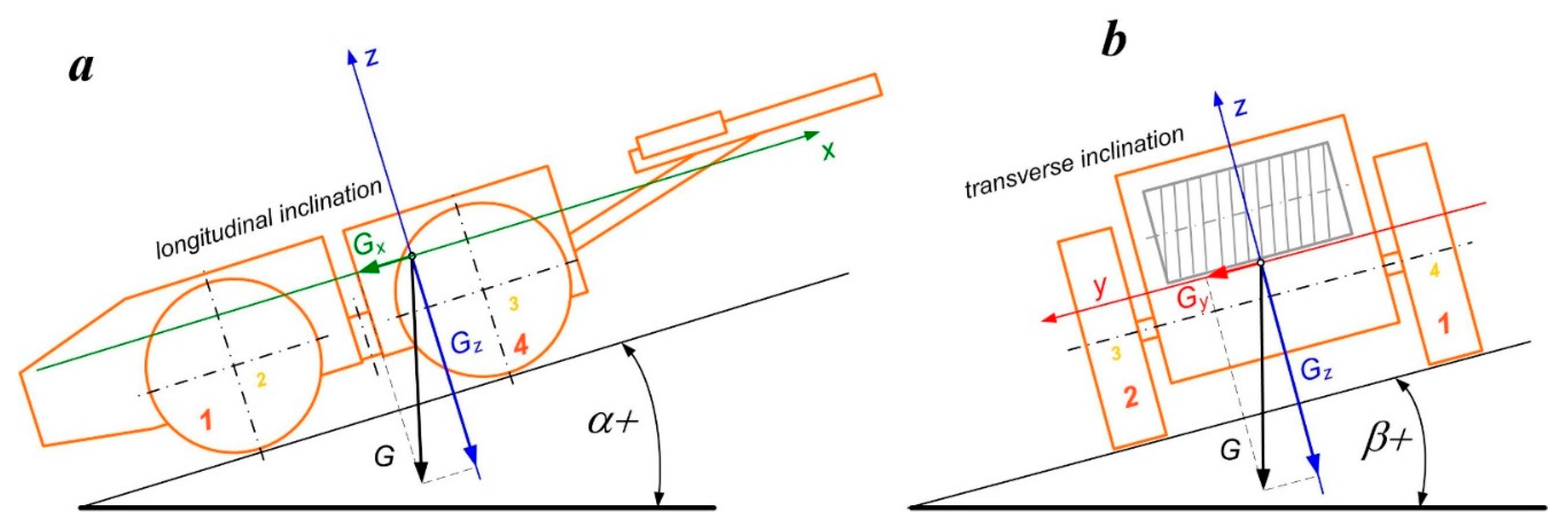
3.3. Influence of the Longitudinal and Transverse Slope of the Excavation

According to the assumptions, the excavation can be inclined on the longitudinally–longitudinal inclination angle α or transversely–transverse inclination angle β. The transverse and longitudinal angles are measured in perpendicular directions, from the vertical (Figure 6). The xyz system is a local system related to the centre of gravity of the analysed self-propelled mining machine. Due to the limited values of the longitudinal (≤20°) and transverse (≤10°) angles, simplified calculations were applied.

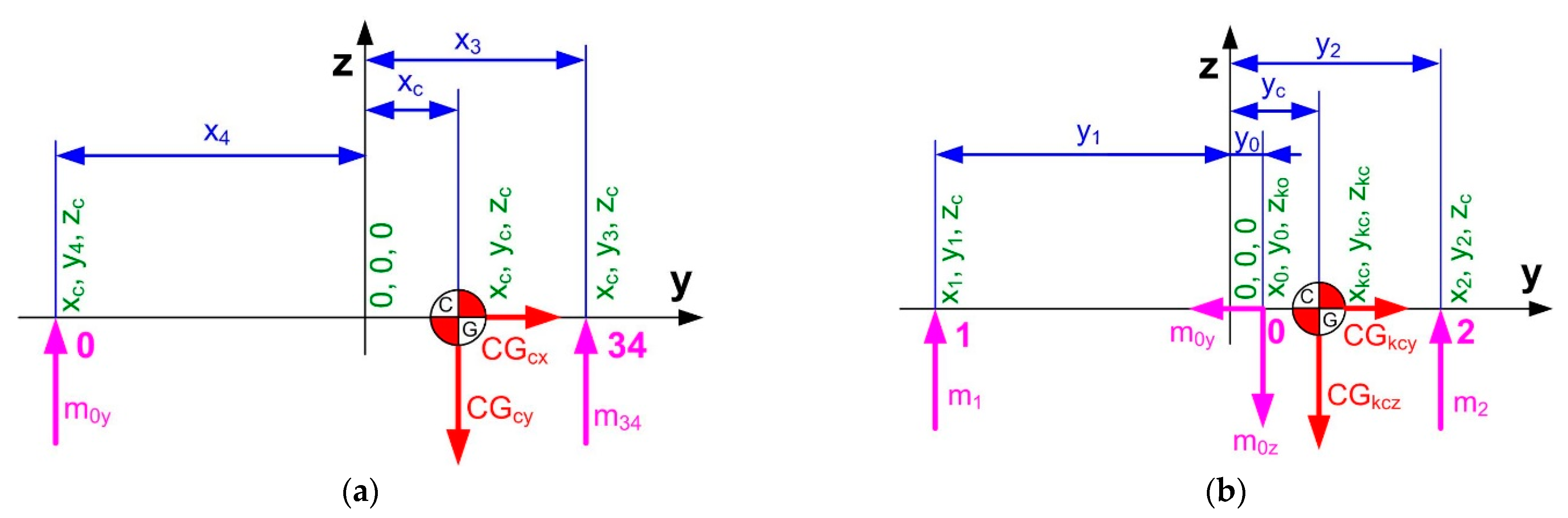
Based on the analysis of the distribution of gravity, formulas for its individual components were expressed as follows:

$$G_x=G\sin \left(\alpha \right)$$

(26)

$$G_y=G\sin \left(\beta \right)$$

(27)

$$\begin{array}{l}{G}_z=G\sqrt{{\cos }^2\left(\alpha \right)-{\sin }^2\left(\beta \right)}\\ \mathrm{or}{G}_z=G\sqrt{{\cos }^2\left(\beta \right)-{\sin }^2\left(\alpha \right)}\end{array}$$

(28)

$$WG=\sqrt{{\cos }^2\left(\beta \right)-{\sin }^2\left(\alpha \right)}$$

(29)

$$G_z=G\cdot WG$$

(30)

For an excavation with a longitudinal and transverse slope, the development of new formulas is required for calculating the pressure of wheels on the floor. When both slopes are considered at the same time, the components of the gravity force of the rear axle with an oscillation axle and the rest of the machine can be expressed as follows:

$$C{G}_{cpwx}=C{G}_{cpw}\cdot \sin \left(\alpha \right)$$

(31)

$$C{G}_{cpwy}=C{G}_{cpw}\cdot \sin \left(\beta \right)$$

(32)

$$C{G}_{cpwz}=C{G}_{cpw}\cdot WG$$

(33)

$$C{G}_{kx}=C{G}_k\cdot \sin \left(\alpha \right)$$

(34)

$$C{G}_{ky}=C{G}_k\cdot \sin \left(\beta \right)$$

(35)

$$C{G}_{kz}=C{G}_k\cdot WG$$

(36)

Knowing the gravity components that load the machine, we can derive the following formulas for the components of forces loading the system and the forces of wheel pressure on the ground (Figure 7, Figure 8 and Figure 9):

$$m_{0z}=\frac{C{G}_{cpwz}\cdot \left(x_3-x_{cpw}\right)+C{G}_{cpwx}\cdot z_{cpw}}{x_3-x_0}$$

(37)

$$m_{0y}=\frac{C{G}_{cpwy}\cdot \left(x_3-x_{cpw}\right)}{x_3-x_0}$$

(38)

$$m_{2n}=\frac{m_{0z}\cdot \left(y_0-y_1\right)+C{G}_{kz}\cdot \left(y_{kc}-y_1\right)+C{G}_{ky}\cdot z_{kc}+m_{0y}\cdot z_{ko}}{y_2-y_1}$$

(39)

$$m_{1n}=C{G}_{kz}+m_{0z}-m_{2n}$$

(40)

$$m_{3n}=\frac{C{G}_{cpwz}\cdot \left(y_{cpw}-y_4\right)+C{G}_{cpwy}\cdot z_{cpw}-m_{0y}\cdot z_{cpw}-m_{0z}\cdot \left(y_0-y_y\right)}{y_3-y_4}$$

(41)

$$m_{4n}=C{G}_{cpwz}-m_{0z}-m_{3n}$$

(42)

3.4. Influence of Emergency Braking

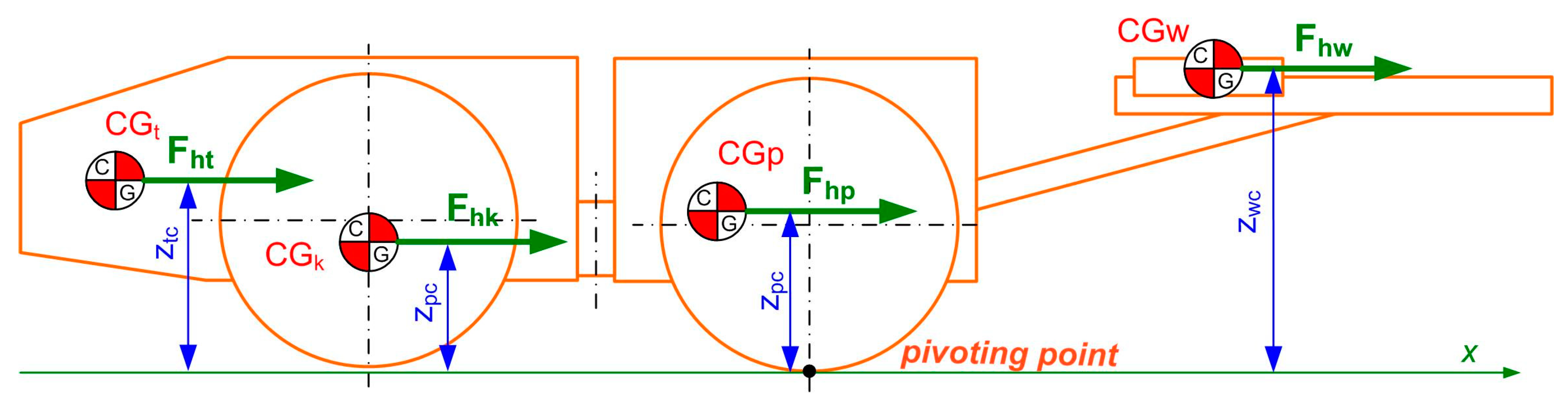
The analysed self-propelled mining machines, due to their long booms, are prone to losing stability in the event of sudden braking. For the needs of this static analytical model, the force of inertia in the case of braking was taken into account. Braking described as braking deceleration a_h acts on each of the centres of gravity, which can be expressed as the M_h braking torque in relation to the axis defined by the contact of wheels 3 and 4 with the floor (Figure 10):

$$M_h=\left(\begin{array}{l}C{G}_t\cdot z_{tc}+C{G}_k\cdot z_{kc}+C{G}_p\cdot z_{pc}+C{G}_{wp}\cdot z_{wpc}\\ +C{G}_{wl}\cdot z_{wlc}\end{array}\right)\cdot a_h$$

(43)

The above formula is identical to the formula describing the action of the same deceleration on the centre of gravity of the entire machine, which allows the braking force and the braking torque to be expressed as follows:

$$F_h=C{G}_c\cdot a_h$$

(44)

$$M_h=F_h\cdot z_c$$

(45)

The braking force was considered as a static force represented by the m_h mass suspended on the Δw_h arm (x_h global coordinate) in the xz plane of the system so that its influence could be taken into account in a simplified manner while ignoring the moments of inertia and the full dynamic model:

$$x_h=l_p+\Delta w_h$$

(46)

$$m_h=\frac{M_h}{\Delta w_h\cdot g}$$

(47)

Therefore, the location of the apparent centre of gravity of the entire machine while taking into account the influence of braking can be expressed as follows:

$$x_{ch}=\frac{C{G}_t\cdot x_{tc}+C{G}_p\cdot x_{pc}+C{G}_k\cdot x_{kc}+C{G}_{wp}\cdot x_{wpc}+C{G}_{wl}\cdot x_{wlc}+m_h\cdot x_h}{C{G}_t+C{G}_p+C{G}_k+C{G}_{wp}+C{G}_{wl}+m_h}$$

(48)

$$y_{ch}=\frac{C{G}_t\cdot y_{tc}+C{G}_p\cdot y_{pc}+C{G}_k\cdot y_{kc}+C{G}_{wp}\cdot y_{wpc}+C{G}_{wl}\cdot y_{wlc}+m_h\cdot y_h}{C{G}_t+C{G}_p+C{G}_k+C{G}_{wp}+C{G}_{wl}+m_h}$$

(49)

$$z_{ch}=\frac{C{G}_t\cdot z_{tc}+C{G}_p\cdot z_{pc}+C{G}_k\cdot z_{kc}+C{G}_{wp}\cdot z_{wpc}+C{G}_{wl}\cdot z_{wlc}+m_h\cdot z_h}{C{G}_t+C{G}_p+C{G}_k+C{G}_{wp}+C{G}_{wl}+m_h}$$

(50)

Next, the location of the CG_cpwh mass and the apparent centre of gravity of the rear body, platform, and boom assembly can be expressed as follows:

$$x_{ch}=\frac{C{G}_t\cdot x_{tc}+C{G}_p\cdot x_{pc}+C{G}_{wp}\cdot x_{wpc}+C{G}_{wl}\cdot x_{wlc}+m_h\cdot x_h}{C{G}_t+C{G}_p+C{G}_{wp}+C{G}_{wl}+m_h}$$

(51)

$$y_{ch}=\frac{C{G}_t\cdot y_{tc}+C{G}_p\cdot y_{pc}+C{G}_{wp}\cdot y_{wpc}+C{G}_{wl}\cdot y_{wlc}+m_h\cdot y_h}{C{G}_t+C{G}_p+C{G}_{wp}+C{G}_{wl}+m_h}$$

(52)

$$z_{ch}=\frac{C{G}_t\cdot z_{tc}+C{G}_p\cdot z_{pc}+C{G}_{wp}\cdot z_{wpc}+C{G}_{wl}\cdot z_{wlc}+m_h\cdot z_h}{C{G}_t+C{G}_p+C{G}_{wp}+C{G}_{wl}+m_h}$$

(53)

$$C{G}_{cpwh}=C{G}_t+C{G}_p+C{G}_{wp}+C{G}_{wl}+m_h$$

(54)

Knowing the gravity components that load the machine, we can derive the following formulas for the components of forces loading the system and the forces of wheel pressure on the ground:

$$m_{0h}=\frac{x_3-x_{ch}}{x_3-x_0}\cdot C{G}_{cpwh}$$

(55)

$$m_{3h}=\frac{C{G}_{cpwh}\cdot \left(y_{ch}-y_4\right)-m_{0h}\cdot \left(y_0-y_4\right)}{y_3-y_4}$$

(56)

$$m_{4h}=C{G}_{cpwh}-m_{0h}-m_{3h}$$

(57)

$$m_{2h}=\frac{m_{0h}\cdot \left(y_0-y_1\right)+C{G}_k\cdot \left(y_{kc}-y_1\right)}{y_2-y_1}$$

(58)

$$m_{1h}=C{G}_k+m_{0h}-m_{2h}$$

(59)

3.5. Influence of Driving over a Drop

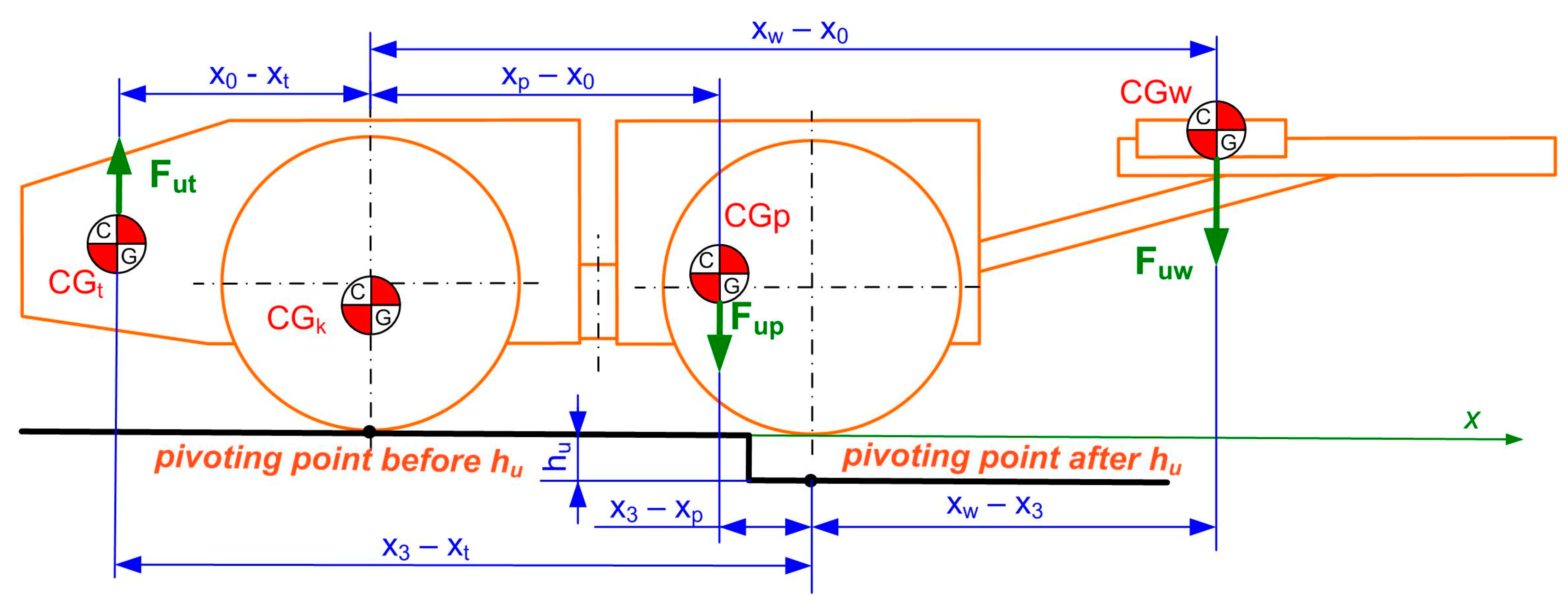
Driving on an uneven floor was considered as driving over a perpendicular drop with the h_u height from which the front axle falls, generating a dynamic force in the centre of gravity of each subassembly (Figure 11). The pivot point of the machine in this case is the axis going through the point of contact of wheels 1 and 2 with the floor. When the front axle hits against the floor, the machine tries to rotate, due to the M_up torque overbalancing the machine in relation to the axis going through the points of contact of wheel 3 and 4 with the floor. Due to the slight rotation, it was assumed that the forces act perpendicularly despite the fact that the rig moves on an arc. Additionally, the M_ub torque that overbalances the machine to the sides can be determined. The presented derivation takes into account several assumptions and simplifications, which enables a quick calculation of the impact of the drop. However, it should be corrected at the stage of simulation or empirical dynamic tests, especially with respect to damping and the effect of smooth driving over a drop instead of the assumed sudden impact.

Depending on the distance of the centre of gravity from the axis of rotation 1–2, the corrected equivalent mass of the machine can be expressed as follows (Figure 11):

$$\begin{array}{ll}\hfill m_{zast}=C{G}_t\cdot \frac{x_{tc}-x_{sr}}{x_3-x_{sr}}& +C{G}_k\cdot \frac{x_{kc}-x_{sr}}{x_3-x_{sr}}+C{G}_p\cdot \frac{x_{pc}-x_{sr}}{x_3-x_{sr}}\hfill \\ & +C{G}_{wp}\cdot \frac{x_{wpc}-x_{sr}}{x_3-x_{sr}}+C{G}_{wl}\cdot \frac{x_{wlc}-x_{sr}}{x_3-x_{sr}}\hfill \end{array}$$

(60)

where x_sr is identical to point x₀, but it can also be expressed as:

$$x_{sr}=\frac{x_1+x_2}{2}$$

(61)

For the equivalent mass described in this way and the h_u height of the drop, the energy of the machine when the wheels are in contact with the floor can be expressed as:

$$E_{ku}=m_{zast}\cdot g\cdot h_u$$

(62)

When the wheels are in contact with the floor, the machine energy is converted into the potential energy of wheel elasticity, which for k_o = 2*k_opony, stiffness can be expressed as follows:

$$E_{ps}=\frac{k_o\cdot x_{uop}^2}{2}$$

(63)

It should be noted that tyre deflection means that the machine represented as an equivalent mass is lowered by this deflection, releasing additional potential energy:

$$E_{pu}=m_{zast}\cdot g\cdot x_{uop}$$

(64)

Hence, the energy equivalence can be expressed as follows:

$$E_{ps}=E_{pu}+E_{ku}$$

(65)

By substituting appropriate formulas and performing transformations, the following equation of a quadratic function can be obtained:

$$k_o\cdot x_{uop}^2-2\cdot m_{zast}\cdot g\cdot x_{uop}-2\cdot m\cdot g\cdot h_u=0$$

(66)

The solution of this quadratic equation provides a deflection formula. Due to the physical interpretation and the assumptions made, only a positive result is acceptable:

$$x_{uop}=\frac{m_{zast}\cdot g+\sqrt{m_{zast}^2\cdot g^2+2\cdot k_o\cdot m_{zast}\cdot g\cdot h_u}}{k_o}$$

(67)

Knowing the value of deflection and assuming a linear relationship between the force and the deflection, which is correct near this point, we can express the formula for the force acting on the front axle of the rig as follows:

$$F_u=k_o\cdot x_{uop}$$

(68)

Therefore, it is possible to calculate the a_u deceleration acting on the rig as follows:

$$a_{usk}=\frac{F_u}{m_{zast}}$$

(69)

It is deceleration caused by springs and must be reduced by the value of gravitational acceleration g so as to obtain the resultant deceleration. In addition, the formulas were corrected so that for a given zero value of the drop, its effect would be equal to zero. Thus, it was possible to eliminate the influence of gravity, which is taken into account separately when calculating the location of the centre of gravity. Due to the different distances of the centres of gravity from the axis of rotation 1–2, the factor determining the influence of this distance should be calculated as follows:

$$i_{ut}=\frac{a_{usk}}{g}\cdot \frac{x_{tc}-x_{sr}}{x_3-x_{sr}}$$

(70)

$$i_{uk}=\frac{a_{usk}}{g}\cdot \frac{x_{kc}-x_{sr}}{x_3-x_{sr}}$$

(71)

$$i_{up}=\frac{a_{usk}}{g}\cdot \frac{x_{pc}-x_{sr}}{x_3-x_{sr}}$$

(72)

$$i_{uwp}=\frac{a_{usk}}{g}\cdot \frac{x_{wpc}-x_{sr}}{x_3-x_{sr}}$$

(73)

$$i_{uwl}=\frac{a_{usk}}{g}\cdot \frac{x_{wlc}-x_{sr}}{x_3-x_{sr}}$$

(74)

Knowing the masses and coordinates of the centres of gravity and the above presented coefficients, we can derive a formula for the torque attempting to overbalance the machine in relation to axis 3–4 as follows:

$$M_{up}=g\cdot \left(\begin{array}{l}-C{G}_t\cdot \left(x_3-x_{tc}\right)\cdot i_{ut}-C{G}_k\cdot \left(x_3-x_{kc}\right)\cdot i_{uk}\\ -C{G}_p\cdot \left(x_3-x_{pc}\right)\cdot i_{up}+C{G}_{wp}\cdot \left(x_{wpc}-x_3\right)\cdot i_{uwp}\\ +C{G}_{wl}\cdot \left(x_{wlc}-x_3\right)\cdot i_{uwl}\end{array}\right)$$

(75)

Additionally, the formula for the torque overbalancing the rig to the side is:

$$M_{ub}=g\cdot \left(\begin{array}{l}-C{G}_t\cdot y_{tc}\cdot i_{ut}-C{G}_k\cdot y_{kc}\cdot i_{uk}-C{G}_p\cdot y_{pc}\cdot i_{up}\\ -C{G}_{wp}\cdot y_{wpc}\cdot i_{uwp}-C{G}_{wl}\cdot y_{wlc}\cdot i_{uwl}\end{array}\right)$$

(76)

Another problem was determining the effect of the drop on the machine’s behaviour when the set value of the drop is lower than the static deflection of the front axle (mean deflection of the front wheels). In such a case, despite the existence of a drop, the tyres are still resiliently deformed. Therefore, the above quadratic equation was derived for respective energy values at the beginning and end of the drop phase.

The Δz_p front axle deflection as the mean deflection of both tyres can be expressed as follows:

$$\Delta z_p=\frac{\Delta z_3+\Delta z_4}{2}$$

(77)

For the h_u < Δz_p drop height, we can write the machine’s potential energy, which is converted into the potential energy of wheel elasticity. It should be noted, however, that the tyres are initially deflected, and this deflection stores the elastic energy in the tyres. Taking the above into account, the equivalence can be expressed as follows:

$$m_{zast}\cdot g\cdot \left(x_u-\Delta z_p+h_u\right)+\frac{k_o\cdot {\left(\Delta z_p-h_u\right)}^2}{2}=\frac{k_o\cdot x_u^2}{2}$$

(78)

The respective formulas are used depending on whether the drop is greater than the deflection of the front axle.

As before, the torque caused by the drop was considered as a static force represented by the m_u mass suspended on the Δw_u arm (x_u global coordinate) in the xz plane of the system:

$$x_u=\Delta w_u+l_p$$

(79)

$$m_u=\frac{M_{up}}{\Delta w_u\cdot g}$$

(80)

Knowing the m_u mass and the M_ub torque, we calculated the y_u coordinate of this mass. Therefore, similarly to the previous considerations, the location of the apparent centre of gravity of the entire machine while taking into account the braking effect can be expressed as follows:

$$x_{cu}=\frac{C{G}_t\cdot x_{tc}+C{G}_p\cdot x_{pc}+C{G}_k\cdot x_{kc}+C{G}_{wp}\cdot x_{wpc}+C{G}_{wl}\cdot x_{wlc}+m_u\cdot x_u}{C{G}_t+C{G}_p+C{G}_k+C{G}_{wp}+C{G}_{wl}+m_u}$$

(81)

$$y_{cu}=\frac{C{G}_t\cdot y_{tc}+C{G}_p\cdot y_{pc}+C{G}_k\cdot y_{kc}+C{G}_{wp}\cdot y_{wpc}+C{G}_{wl}\cdot y_{wlc}+m_u\cdot y_u}{C{G}_t+C{G}_p+C{G}_k+C{G}_{wp}+C{G}_{wl}+m_u}$$

(82)

$$z_{cu}=\frac{C{G}_t\cdot z_{tc}+C{G}_p\cdot z_{pc}+C{G}_k\cdot z_{kc}+C{G}_{wp}\cdot z_{wpc}+C{G}_{wl}\cdot z_{wlc}+m_u\cdot z_u}{C{G}_t+C{G}_p+C{G}_k+C{G}_{wp}+C{G}_{wl}+m_u}$$

(83)

Next, the CG_cpwu masses and the apparent centre of gravity of the rear body, platform, and booms assembly were calculated:

$$x_{cu}=\frac{C{G}_t\cdot x_{tc}+C{G}_p\cdot x_{pc}+C{G}_{wp}\cdot x_{wpc}+C{G}_{wl}\cdot x_{wlc}+m_u\cdot x_u}{C{G}_t+C{G}_p+C{G}_{wp}+C{G}_{wl}+m_u}$$

(84)

$$y_{cu}=\frac{C{G}_t\cdot y_{tc}+C{G}_p\cdot y_{pc}+C{G}_{wp}\cdot y_{wpc}+C{G}_{wl}\cdot y_{wlc}+m_u\cdot y_u}{C{G}_t+C{G}_p+C{G}_{wp}+C{G}_{wl}+m_u}$$

(85)

$$z_{cu}=\frac{C{G}_t\cdot z_{tc}+C{G}_p\cdot z_{pc}+C{G}_{wp}\cdot z_{wpc}+C{G}_{wl}\cdot z_{wlc}+m_u\cdot z_u}{C{G}_t+C{G}_p+C{G}_{wp}+C{G}_{wl}+m_u}$$

(86)

$$C{G}_{cpwu}=C{G}_t+C{G}_p+C{G}_{wp}+C{G}_{wl}+m_u$$

(87)

Knowing the gravity components that load the machine, we can derive the following formulas for the components of forces loading the system and the forces of the wheel pressure on the ground:

$$m_{0u}=\frac{x_3-x_{cu}}{x_3-x_0}\cdot C{G}_{cpwu}$$

(88)

$$m_{3u}=\frac{C{G}_{cpwu}\cdot \left(y_{ch}-y_4\right)-m_{0u}\cdot \left(y_0-y_4\right)}{y_3-y_4}$$

(89)

$$m_{4u}=C{G}_{cpwu}-m_{0u}-m_{3u}$$

(90)

$$m_{2u}=\frac{m_{0u}\cdot \left(y_0-y_1\right)+C{G}_k\cdot \left(y_{kc}-y_1\right)}{y_2-y_1}$$

(91)

$$m_{1u}=C{G}_k+m_{0u}-m_{2u}$$

(92)

3.6. Determining the Pressure of Jacks on the Floor

In the working position, the drilling rig is directed straight ahead and placed on jacks. Hydraulic jacks level the rig in the excavation. From the point of view of statics, a rigid body with four parallel jacks is a statically indeterminable system. The values of jack pressures on the floor were determined by a unique graphic method, which is correct for a rectangle [35]. Therefore, the model assumes the height of the rectangle as the average spacing of jacks. It should be noted that this is a favourable assumption, because increasing the spacing of the front jacks increases the stability of the machine, so the analysis concerns a less favourable case.

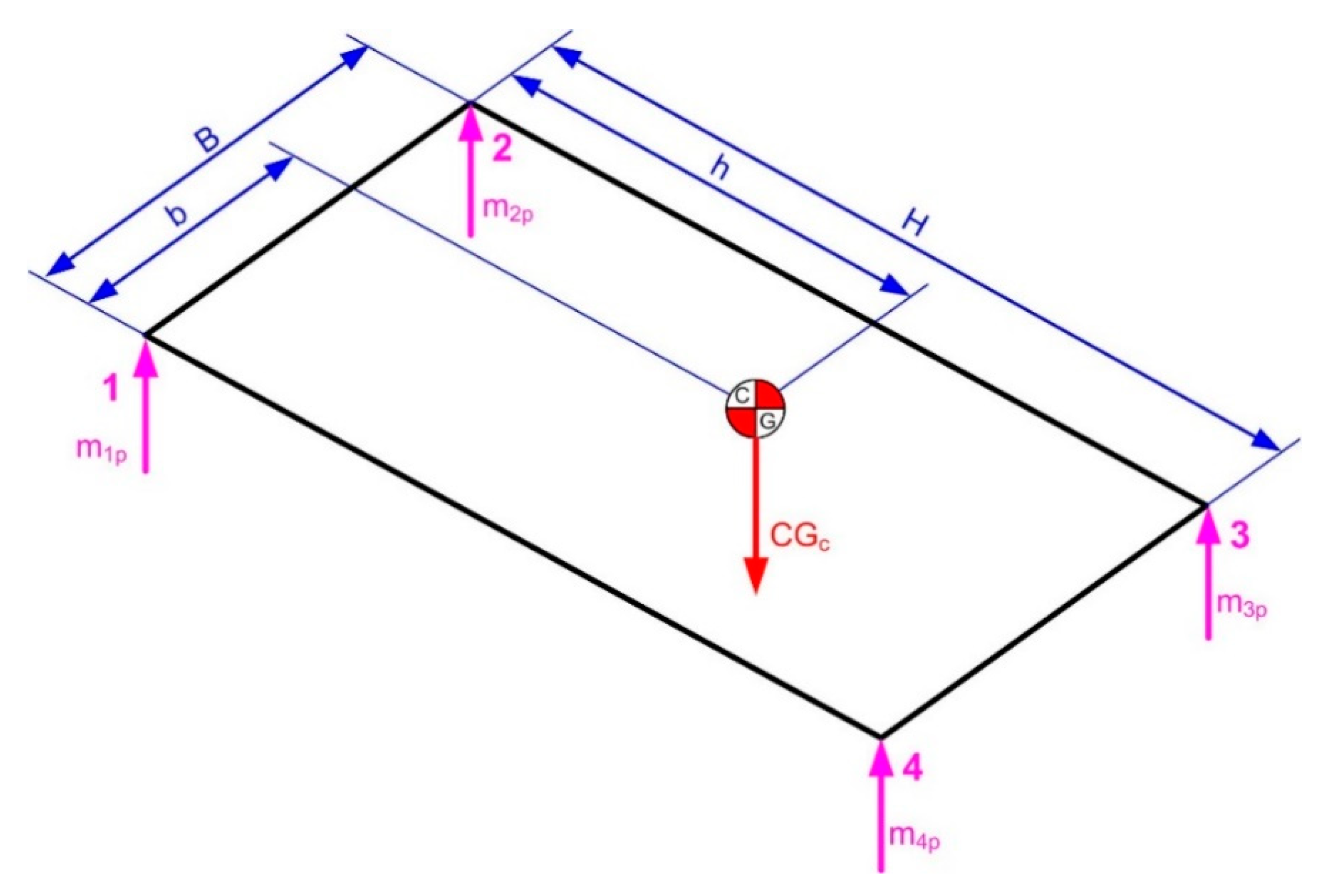
The rectangle with a height H and length B is supported at four points on the ground. Inside the outline of this rectangle, it is acted on by a perpendicular force applied at the point having coordinates b and h, with point 0.0 being described in the lower left corner. For the so-adopted system, assuming the consistency of the denotations adopted in this study, formulas for H, B, h, and b (Figure 12) can be expressed as follows:

$$H=\frac{b_{pt}+b_{pp}}{2}$$

(93)

$$B=l_{pt}+l_{pp}$$

(94)

$$h=y_c+\frac{H}{2}$$

(95)

$$b=x_c+l_{pt}$$

(96)

Hence, it is possible to calculate the pressure of jacks on the floor from the following formulas:

$$m_{1p}=C{G}_c\cdot \frac{\left(B-b\right)\left(H-h\right)}{H\cdot B}$$

(97)

$$m_{2p}=C{G}_c\cdot \frac{\left(B-b\right)\cdot h}{H\cdot B}$$

(98)

$$m_{3p}=C{G}_c\cdot \frac{b\cdot h}{H\cdot B}$$

(99)

$$m_{4p}=C{G}_c\cdot \frac{\left(H-h\right)\cdot b}{H\cdot B}$$

(100)

3.7. Computational Model and Spreadsheet

Based on the above considerations and formulas derived, a uniform theoretical model was created, taking into account the influence of all factors. The theoretical model was saved in the form of a transparent spreadsheet in MathCad. Next, a spreadsheet in Microsoft Excel was developed. For the purpose of calculating additional quantities, formulas describing the tipping edges or the distance of the centre of gravity from the tipping edge, the generally known mathematical relationships were applied. As a result, an easy-to-use calculation sheet was obtained, which, after entering a number of values, enables evaluation of the stability of drilling rigs for several variables and parameters. In the next step, the computational model and the spreadsheet were verified and validated based on the example of a specific drilling vehicle.

4. Verification and Validation of the Developed Model

The computational model was verified and validated on the basis of data concerning the Mine Master Face Master 2.8 drilling rig (hereinafter referred to as FM 2.8).

Verification and validation were performed by comparing the results with those obtained for the dynamic model, the Dynamic Simulation module in Autodesk Inventor Professional programme and empirical tests on truck scales.

4.1. Parameters of the Analysed Drilling Rig

Verification and validation were carried out for the FM 2.8 twin-boom drilling rig, for which all the necessary values are listed in the tables below (

Table 1. Geometric sizes of FM 2.8.

Machine Geometry–Parameters
No.	Quantity	Denotation	Value [mm]
1.	Total width of the machine	bc	2250
2.	Front wheel track	bp	1900
3.	Front axle distance	lp	1650
4.	Rear wheel track	bt	1900
5.	Rear axle distance	lt	1650
6.	Front jacks spacing	bpp	1900/2800
7.	Front jacks distance	lpp	2500
8.	Rear jacks spacing	bpt	1900
9.	Rear jacks distance	lpt	2500
10.	Boom joint spacing	bw	1500
11.	Distance of boom joints α	lwα	2000
12.	Distance of boom joints β	lwα	1800
13.	Boom joint height	zw	1800
14.	Wheel outer radius	R	600

,

Table 2. Mass of FM 2.8 components.

Centres of Gravity of the Machine Components–Mass
No.	Component	Denotation	Value [kg]
1.	Rear body without the oscillation axle assembly	CGt	12,500
2.	Platform	CGp	6900
3.	Oscillation axle assembly	CGk	1700
4.	Right = left boom	CGw	3570

,

Table 3. Location of the centres of gravity of PM 2.8 components.

Centres of Gravity of Machine Components–Location
No.	Component	Denotation	x [mm]	y [mm]	z [mm]
1.	Rear body without the oscillation axle assembly	CGt–xt, yt, zt	500	20	1350
2.	Platform	CGp–xp, yp, zp	−540	−10	1300
3.	Oscillation axle assembly	CGk–xk, yk, zk	0	−50	600
4.	Right = left boom–min	CGw–lwmin	2650
5.	Right = left boom–max	CGw–lwmax	3650
6.	Right = left boom–max	CGw–hw	300

and

Table 4. Variables of FM 2.8 components.

Machine Kinematics–Variables
No.	Quantity	Denotation	Range
1.	Machine turning angle	γ	−40°–+40°
2.	Boom lift	αw	−25°–+45°
3.	Boom swing	βw	−35°–+35° −55°–+55°-for αw+ = max
4.	Telescopic jib extension	Δw	0–1350 mm

).

4.2. Verification of the Theoretical Model

By substituting the data for FM 2.8, several hundred simulations were carried out to analyse the influence of individual data on the obtained results. In particular, typical situations, such as the turning of the machine and the rotation of the booms, were analysed. Next, the influences of the longitudinal and transverse slope, braking, and drop were analysed.

The results provided by the model in question are consistent with the results obtained from the full dynamic model (

Table 5. Distribution of wheel pressures: comparison of results provided by the AGH model and the full dynamic model.

No.	Configuration	Model	m1 [kg]	m2 [kg]	m3 [kg]	m4 [kg]
1.	Machine straight ahead Booms straight ahead	AGH	5879	5798	8339	8191
2.		Dynamic	5856	5780	8362	8210
3.	Machine 40° to the right Booms straight ahead	AGH	5485	5404	4776	12,544
4.		Dynamic	5655	5239	4723	12,591
5.	Machine 40° to the left Booms 15° to the left	AGH	5551	5470	14,915	2271
6.		Dynamic	5232	5809	15,190	1987

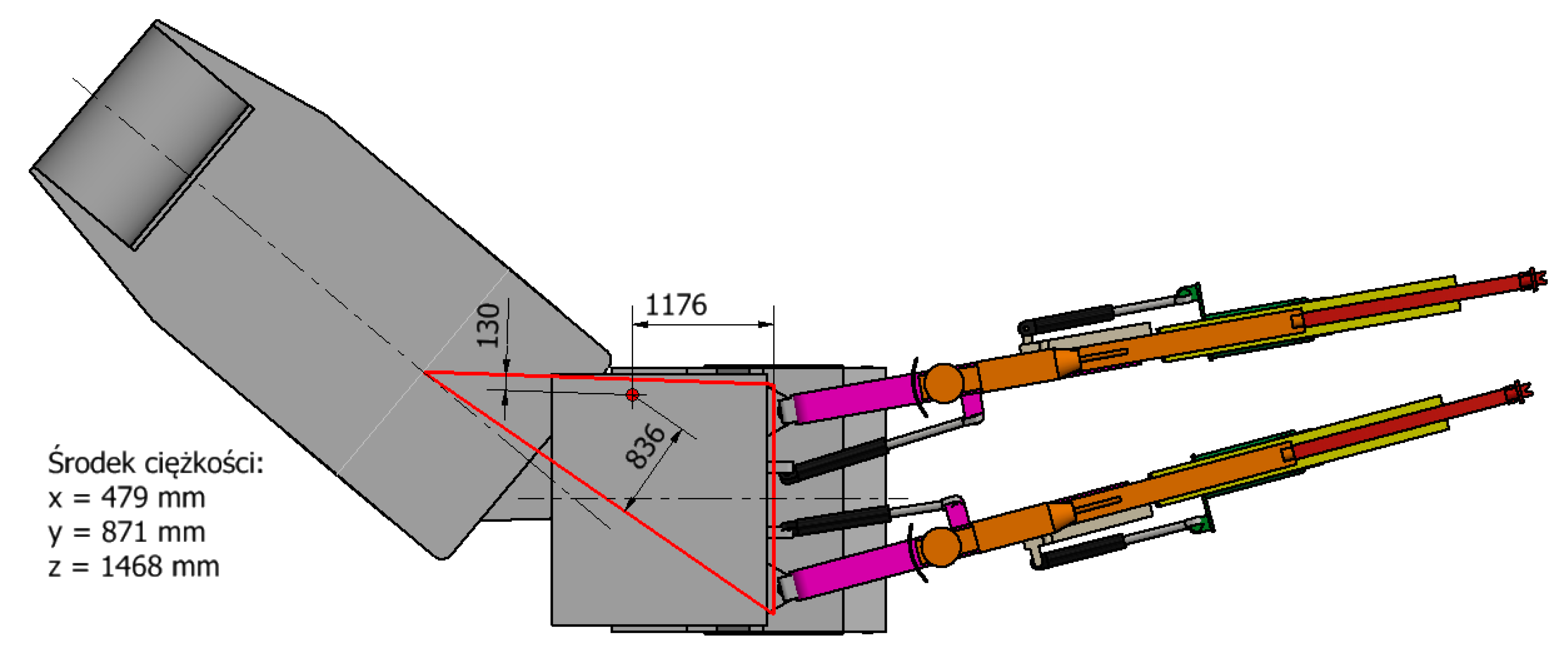
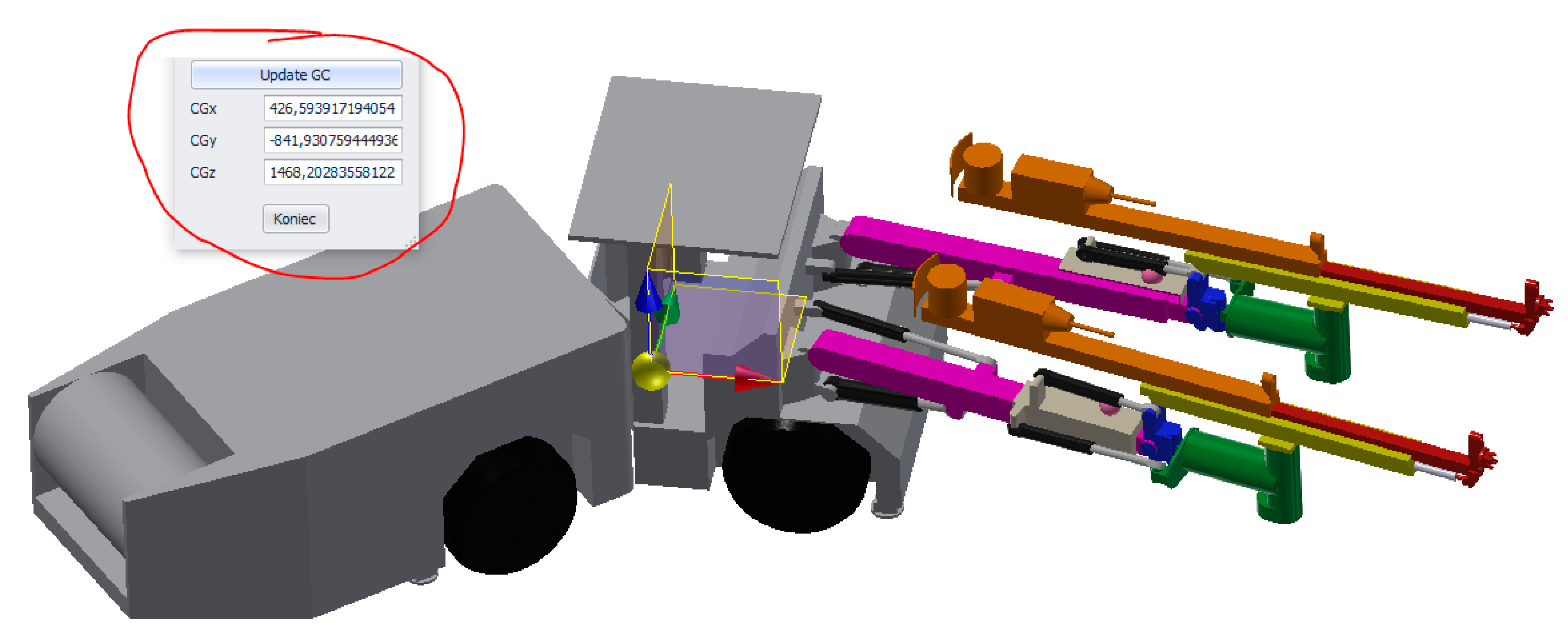
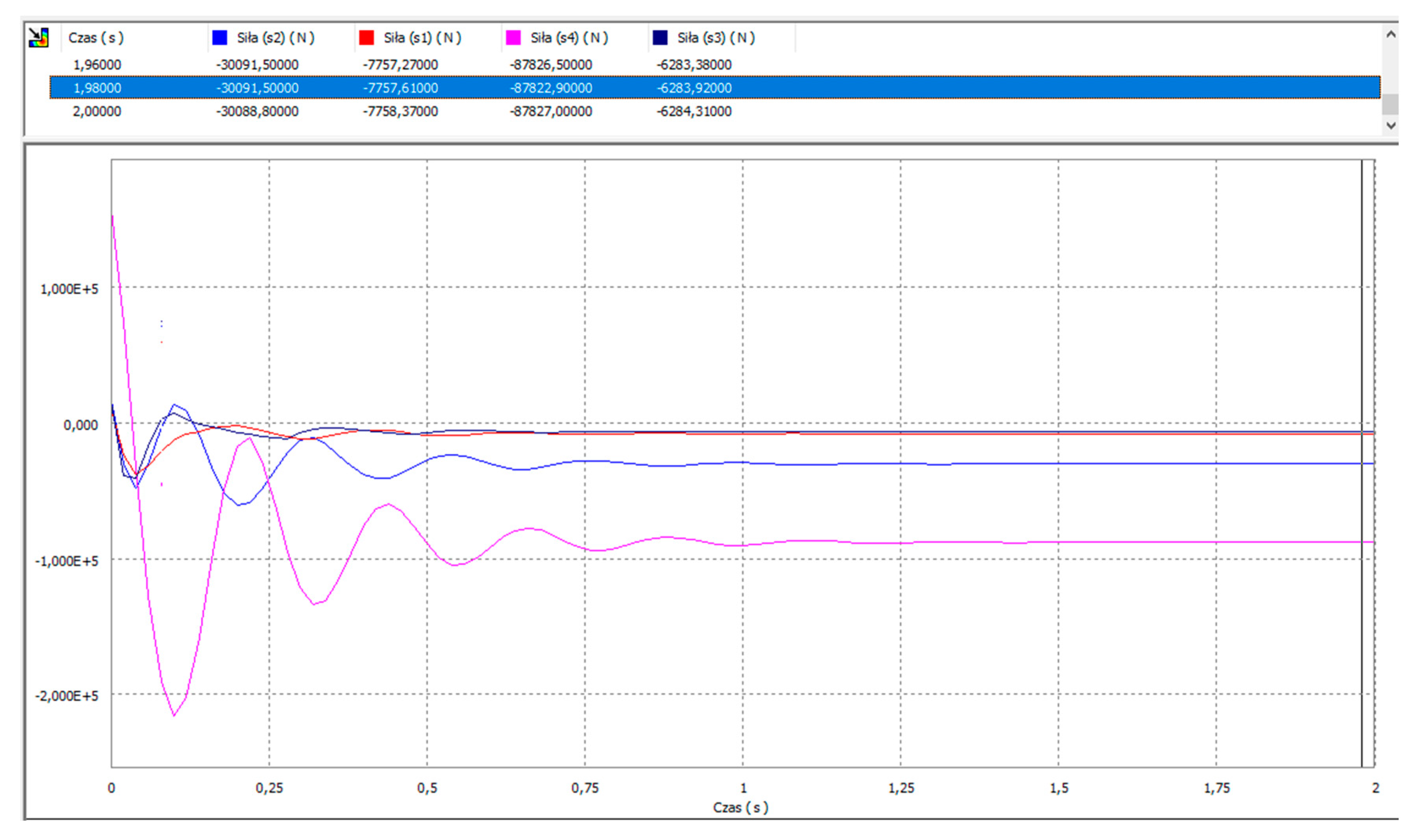
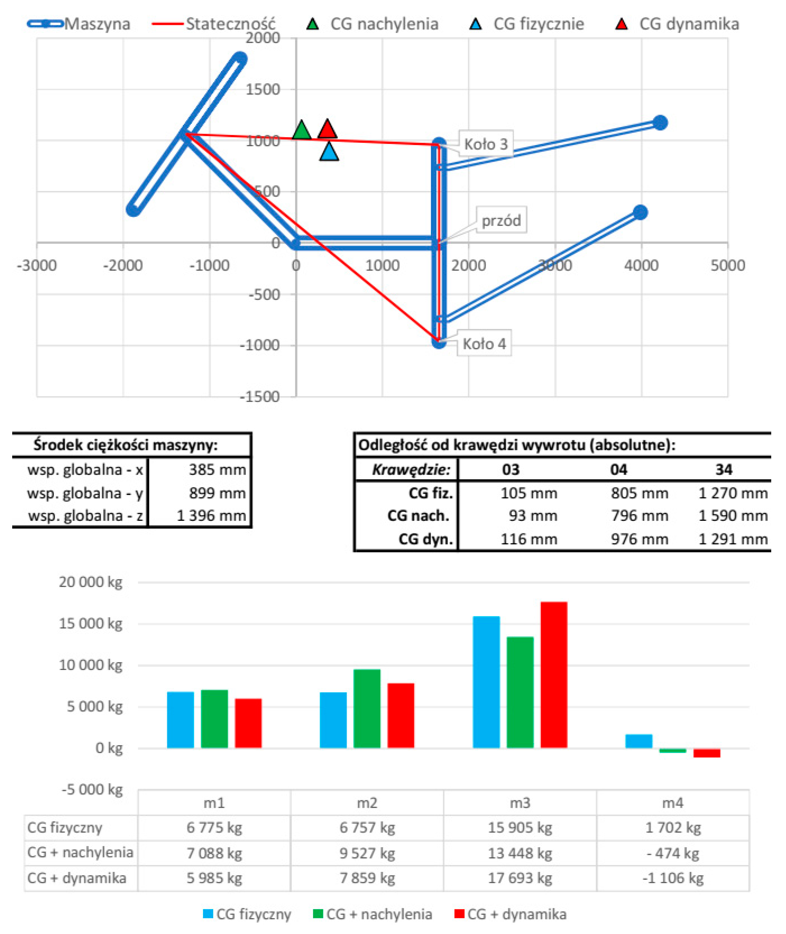
). Additionally, special models were created for the needs of model studies in Dynamic Simulation in Autodesk Inventor Professional programme. The obtained results correspond with those provided by the developed model. Figure 13 and Figure 14 show examples of analyses of the location of the centre of gravity. Figure 15 presents examples of the results of a dynamic simulation of wheel pressure on the ground, whereas Figure 16 shows examples of results calculated by the developed spreadsheet. Apart from the graphic interpretation of the arrangement of the machine and booms, the location of the centre of gravity, wheel pressure values, and distance of the centre of gravity from the tipping edge are shown. In the presentation of the pressures and the centre of gravity, the influence of the excavation slope and dynamic forces was taken into account. Figure 16 shows the machine diagram in blue and the tipping edges in red. Additionally, the centre of gravity is marked with triangles and the values of individual wheel’s pressure are presented in the bar chart. The blue colour corresponds to the location of the centre of gravity and the values for the horizontal excavation, the green colour for the inclined excavation, whereas the red one refers to the values regarding the inclined excavation and the influence of the braking inertia force and driving over a drop.

4.3. Validation of the Theoretical Model

In the last stage, the model was validated with the data obtained during tests on truck scales (Figure 17). Validation was carried out for the pressure of wheels (Figure 17a) and jacks (Figure 17b) on the ground.

The calculations were performed for the FM 2.8 data and compared with the results obtained during the tests in the following comparable cases:

• Machine straight ahead, booms straight ahead (

  Table 6. Comparison of the results of the model and empirical tests: machine and booms straight ahead.

  No.	Component	m1 [kg]	m2 [kg]	m3 [kg]	m4 [kg]
  1.	Measurement on scales	6780	6760	8700	7900
  2.	Theoretical model	6775	6758	8 710	7897
  Absolute error [kg]		5	2	−10	3
  Relative error [%]		0.07%	0.03%	−0.11%	0.04%

  );
• Machine turned 40° to the left, booms straight ahead (

  Table 7. Comparison of the results of the model and empirical tests: chassis turned to the left, booms straight ahead.

  No.	Component	m1 [kg]	m2 [kg]	m3 [kg]	m4 [kg]
  1.	Measurement on scales	6090	6440	13,810	3760
  2.	Theoretical model	6171	6153	13,733	4084
  Absolute error [kg]		−81	287	77	−324
  Relative error [%]		−1.33%	4.46%	0.56%	−8.62%

  );
• Machine turned 40° to the left, booms turned 15° to the left (

  Table 8. Comparison of the results of the model and empirical tests: chassis turned to the left, booms to the left.

  No.	Component	m1 [kg]	m2 [kg]	m3 [kg]	m4 [kg]
  1.	Measurement on scales	6140	6430	15,600	1930
  2.	Theoretical model	6278	6263	15,999	1603
  Absolute error [kg]		−138	167	−399	327
  Relative error [%]		−2.25%	2.60%	−2.56%	16.94%

  ).

The results provided by the theoretical model are consistent with the results of the empirical research. The results of the jack pressure obtained during empirical tests cannot be considered reliable. Due to the design of the machine, it is possible to obtain different pressures depending on the extension of the jacks. The centre of gravity of the machine is not in the geometric centre of the jacks, so in an extreme case, one of the jacks may not be in contact with the ground and the machine is still stable. The analysis of the results obtained during empirical studies and their comparison with the wheel pressures on the ground from the same empirical studies clearly indicate that they are not fully consistent (

Table 9. Comparison of the pressure of wheels and jacks from the empirical and model tests.

No.	Component	m1 [kg]	m2 [kg]	m3 [kg]	m4 [kg]
1.	Jack pressure–measurement on scales	7990	6220	9190	6790
2.	Wheel pressure–measurement on scales	6780	6760	8700	7900
3.	Jack pressure–computational model	6721	7087	8382	7951

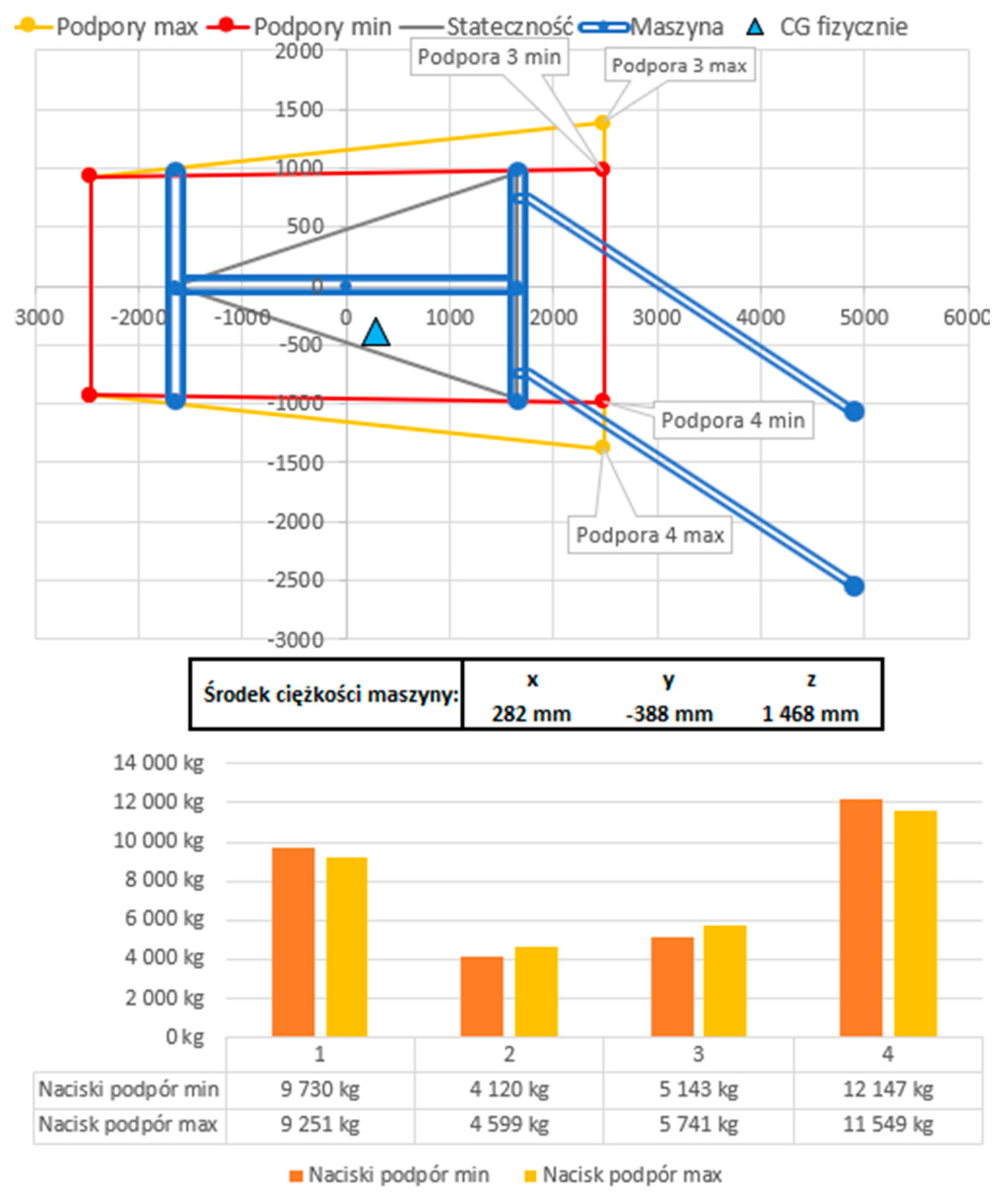
). However, the differences in the results are acceptable for the assessment of the stability of the machine on jacks. Additionally, Figure 18 presents selected results of the stability assessment obtained from the developed spreadsheet. As in the case of Figure 16, the geometry of the machine with booms presented in the graph in Figure 18 is marked in blue. The tipping edges defined by the jacks in the minimum position are marked in red, and in the maximum position in yellow. The bar charts also show the values for jacks in the minimum and maximum positions. The location of the machine’s centre of gravity is marked in the graph with a blue triangle. In the case of an on-site analysis, the machine is placed horizontally.

4.4. Discussion

The presented verification results indicate that the developed model is correct. The values of the coordinates of the centres of gravity and the values of the wheels’ and jacks’ pressure forces change as expected.

A comparison of the calculation and measurement results also confirms the correctness of the model. For the machine straight ahead, the relative error is negligible and slightly exceeds 0.1%. For a twisted machine and tilted booms, the error is greater, reaching nearly 9% and 17%. It is important that the error of 9% and 17% applies to the least loaded wheels, and the absolute error reaches 324 and 327 kg, respectively. The maximum relative error does not exceed 400 kg, which is acceptable for a machine of this mass and for the needs of stability assessment.

It should be clearly emphasized that the error does not result from improper operation of the model, but from inaccurate determination of the mass and the location of the centres of gravity of subassemblies, i.e., the data that affect the calculation results. At the design stage, the mass and the centre of gravity are determined on the basis of the 3D model. However, not all elements are included in the 3D model. For example, the masses of hydraulic oil, lubricant, and fuel are ignored. Moreover, the mass of commercial elements is based on catalogue data, which is sometimes inaccurate.

5. Results of Analytical Tests of the Drilling Rig Stability

Next, qualitative tests were carried out to check whether the model responded correctly to change of the input parameters. In total, several hundred different analyses were conducted for the full computational model with the booms rotating independently in two planes; first, for various combinations of parameters and separate cases, such as horizontal excavation, longitudinally inclined excavation, transversely inclined excavation, braking in a horizontal excavation, drop in a horizontal excavation, and, then, for the listed combinations (

Table 10. Results of selected analyses: wheel pressure-horizontal excavation.

No.	Case	m1 [kg]	m2 [kg]	m3 [kg]	m4 [kg]
1.	Straight ahead, booms straight ahead	6 563	6 545	8 922	8 109
2.	Straight ahead, booms 15° to the left	6 665	6 648	11 503	5 325
3.	Straight ahead, booms 15° to the left, extended	5 638	5 621	13 479	5 402
4.	40° turn to the right, booms straight ahead	6 207	6 190	4 593	13 150
5.	40° turn to the left, booms 15° to the left	6 046	6 028	16 678	1 388
6.	40° turn to the left, 15° to the left, extended	4 883	4 866	20 079	312

,

Table 11. Results of selected analyses: wheel pressure longitudinally inclined excavation.

No.	Case	m1 [kg]	m2 [kg]	m3 [kg]	m4 [kg]
1.	α = 0°, straight ahead, booms straight ahead	6563	6545	8922	8109
2.	α = 12°, straight ahead, booms straight ahead	7781	7764	7365	6570
3.	α = −12°, straight ahead, booms straight ahead	5057	5040	10,089	9294
4.	α = 12°, 40° turn to the left, booms straight ahead	7343	7326	10,677	4136
5.	α = −12°, 40° turn to the right, booms straight ahead	4529	4512	4325	16,115
6.	α = 12°, 40° turn to the right, booms 15° to the right	7728	77,710	2048	11,995

,

Table 12. Results of selected analyses: wheel pressure transversely inclined excavation.

No.	Case	m1 [kg]	m2 [kg]	m3 [kg]	m4 [kg]
1.	β = 0°, straight ahead, booms straight ahead	6563	6545	8922	8109
2.	β = 6°, straight ahead, booms straight ahead	5979	7057	10,288	6651
3.	β = −6°, straight ahead, booms straight ahead	7075	5961	7459	9479
4.	β = 6°, 40° turn to the right, booms straight ahead	5498	6831	6041	11,605
5.	β = −6°, 40° to the right, booms straight ahead	6849	5480	3094	14,551
6.	β = −6°, 40° to the right, booms 15° to the right	6977	5583	458	16,957

,

Table 13. Results of selected analyses: wheel pressure longitudinally and transversely inclined excavation.

No.	Case	m1 [kg]	m2 [kg]	m3 [kg]	m4 [kg]
1.	α = 0°, β = 0°, straight ahead, booms straight ahead	6563	6545	8922	8109
2.	α = −12°, β = 6°, straight ahead, booms straight ahead	4473	5552	11,454	7835
3.	α = −12°, β = 6°, 40° turn to the right, booms straight ahead	3581	4852	18,621	2259
4.	α = −12°, β = 6°, 40° turn to the right, booms 15° to the right	3680	4978	20,973	−318

,

Table 14. Results of selected analyses: wheel pressure braking on an inclined plane.

No.	Case	m1 [kg]	m2 [kg]	m3 [kg]	m4 [kg]
1.	Braking 0 m/s2, α = 0°, β = 0°	6563	6545	8922	8109
2.	Braking 3.5 m/s2, α = 0°, β = 0°	4169	4152	12,129	11,274
3.	Braking 3.5 m/s2, α = 12°, β = 0°	5514	5496	10,428	9592
4.	Braking 3.5 m/s2, α = −12°, β = 0°	2643	2626	13,299	12,463
5.	Braking 3.5 m/s2, α = −12°, β = −6°	2962	2260	11,292	14,339

and

Table 15. Results of selected analyses: wheel pressure–drop, braking on an inclined plane.

No.	Case	m1 [kg]	m2 [kg]	m3 [kg]	m4 [kg]
1.	Drop 0 mm, braking 0 m/s2, α = 0°	6563	6545	8922	8109
2.	Drop 150 mm, braking 0 m/s2, α = 0°	4155	4137	12,242	11,200
3.	Drop 150 mm, braking 0 m/s2, α = 12°	5500	5483	10,539	9519
4.	Drop 150 mm, braking 3.5 m/s2, α = 0°	1761	1744	15,448	14,364
5.	Drop 150 mm, braking 3.5 m/s2, α = 12°	3232	3215	13,602	12,541
6.	Drop 150 mm, braking 3.5 m/s2, α = −12°	214	197	16,620	15,559

). The wheel loads are marked in red when their value had dropped below 1000 kg.

In the first stage of the research, calculations were made for a horizontal excavation (Table 10). In subsequent variants of calculations, different positions of the rig and the booms were taken into account. Only in one case, a pressure below 1000 kg was obtained. However, the setting of the machine in this case, i.e., tilted and extended booms, is not used in practice.

In the next stage, the longitudinal (Table 11) and transverse (Table 12) slopes of the excavation as well as the combinations of both slopes simultaneously (Table 13) were taken into account. Various combinations of parameters were analysed. In the case of longitudinal inclination, the machine was fully stable, regardless of whether it was straight or twisted to the maximum. In the case of the transverse slope and the combination of both slopes, a pressure below 1000 kg was obtained. This occurred when the machine was fully twisted, and the rotation of the booms reached 15°. It is therefore recommended not to exceed the value of 10°.

The last stage of the analyses involved taking into account the inertia force resulting from braking (Table 14) as well as simultaneous braking and driving over a drop (Table 15). The drilling rig does not lose its stability in the event of braking to the deceleration value of 3.5 m/s², even for the longitudinal and transverse slopes of the excavation. However, simultaneous braking and driving over a drop in an inclined excavation causes the pressure of the rear wheels to decrease significantly below 1000 kg. It is therefore advisable to be careful on a road with bumps and drops and to avoid sudden braking under such conditions.

The above simulation test results prove the correct behaviour of the model. With respect to the analysis of driving over a drop, the model needs to be further verified and validated so as to take into account the actual stiffness of wheels.

First, verification of the pressure of jacks on the ground involved assessment of the load of each of the jacks in relation to the load of individual wheels. For the same machine position, the distribution of gravity on the jacks must be identical with that on the wheels. Next, similarly to the verification of pressure on the wheels, typical cases were analysed, i.e., different arrangements of booms (

Table 16. Results of selected analyses: jack pressure.

No.	Case	m1 [kg]	m2 [kg]	m3 [kg]	m4 [kg]
1.	Booms straight ahead, retracted	6721	7087	8382	7950
2.	Booms straight ahead, extended	6030	6358	9111	8641
3.	Booms 15° to the left, retracted	5544	8400	9756	6439
4.	Booms 15° to the left, extended	4602	7971	11,137	6430
5.	Booms 15° to the left, extended	6041	8580	9108	6412
6.	Booms 15° to the left and 30° upward, extended	5182	8250	10,261	6446
7.	Left boom 15° to the left and 30° upward, Right boom 15° to the right and 30° upward, extended	6539	6894	8575	8133

).

The results of the pressure on jacks are predictable. Appropriate rotation or extension of the booms changes the pressure of individual jacks by changing the position of the centre of gravity.

6. Conclusions

The stability of working machines, especially articulated ones, is a serious problem that requires an appropriate approach from the very beginning of the design process. In the case of drilling rigs, we deal not only with an articulated structure, but also with long booms that extend far beyond the undercarriage. Due to the way of manoeuvring in excavations and the arrangement of the booms, the machine may move or work on the verge of stability. The developed methodology for assessing the stability of self-propelled drilling rigs and the spreadsheet created on its basis enable quick and precise analytical tests to be carried out. The methodology was verified in parallel with the developed 3D virtual model in the Autodesk Inventor Professional environment and model tests carried out in the Dynamic Simulation module. Moreover, the results were compared with the results of stability analysis performed on the basis of the full dynamic model and with the results of empirical tests on truck scales. All the obtained results indicate the correctness of the developed computational model. Owing to the elimination of differential equations, the model in question allows a quick assessment of the machine stability as a function of many input parameters to be carried out.

It should be emphasized that the discussed methodology enabled the creation of a spreadsheet with great possibilities in terms of analysing the influence of not only the geometry and mass of the machine components, but also the impact of braking, driving on an uneven floor, the longitudinal and transverse slope of the excavation, as well as analysis of the jack pressure.

The accuracy of the obtained calculation results depends on the accuracy of the entered data. It is therefore necessary to precisely estimate and update the machine geometry, mass values, and the location of the centres of gravity.

One of the basic goals was to develop a universal parametric model that would allow the use of an Excel spreadsheet to obtain results. The calculations made in Excel were compared with those performed in the MathCad spreadsheet in order to eliminate errors. Moreover, the calculation results in Excel were compared with the simulation results in the specialized Autodesk Inventor Professional programme and with the results obtained by independent reports. It was confirmed that the developed model allows use of an Excel spreadsheet instead of specialised software.

The use of the developed spreadsheet does not require specialized software or skills in the field of modelling. The sheet enables determination of the load of wheels and jacks as a function of many important parameters and variables. Additionally, the distances of the centre of gravity from the tipping edge are calculated. The spreadsheet, in addition to numerical values, also shows a graphical representation of the machine, the location of the centre of gravity, the tipping edges, as well as graphs of wheel and jack loads. This information is sufficient to clearly assess whether the machine is stable. Moreover, the sheet enables a quick assessment of how the introduced structural changes affect the stability of the machine. One of the Polish companies producing mining machines, including drilling rigs, uses this calculation methodology and the calculation spreadsheet to assess the stability of the manufactured machines. After several months of use, some changes and improvements were made, enabling development of the second version of the methodology discussed in this article. Currently, work is underway to create a similar methodology and spreadsheet for self-propelled mining machines whose structure of the rear body differs from that in classic drilling rigs.