
A New Prediction Method for the Complete Characteristic Curves of Centrifugal Pumps


Abstract
:1. Introduction
2. Materials and Methods
3. Suter Transformation and COP Analysis of Complete Characteristic Curves
3.1. Suter Transformation
3.2. COPs Analysis

| Serial Number | Specific Speed | Data Source | |
|---|---|---|---|
| US Units | Metric Units (Used in This Paper) | ||
| 1 | 1032 | 20.00 | Ayder [40] |
| 2 | 1089 | 21.10 | Chen [41] |
| 3 | 1320 | 25.60 | Brown [42] |
| 4 | 1496 | 29.00 | Kittredge [43] |
| 5 | 1555 | 30.14 | Chen [41] |
| 6 | 1935 | 37.50 | Kittredge [43] |
| 7 | 3676 | 71.23 | Liu [44] |
| 8 | 4199 | 81.37 | Chen [41] |
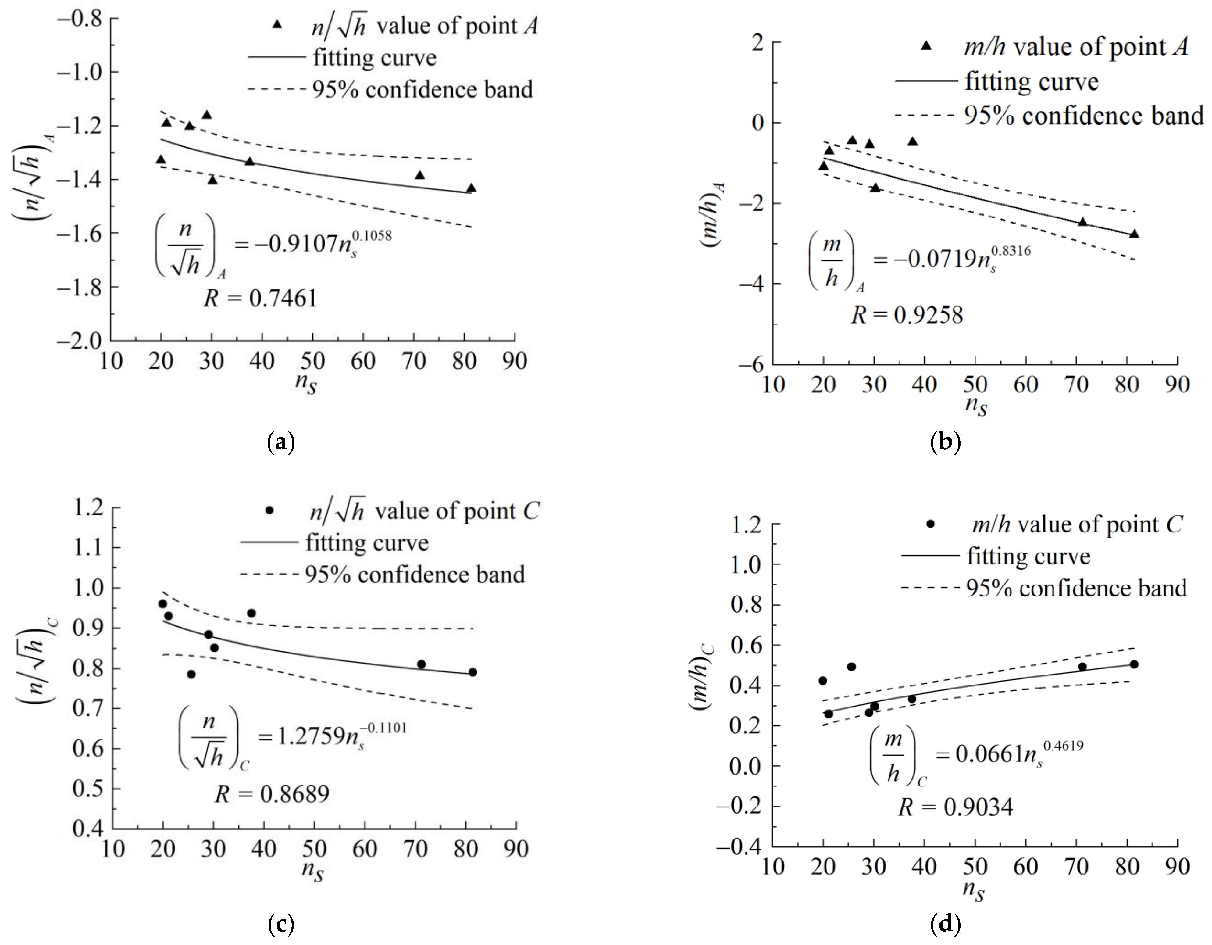
3.2.1. Characteristic Parameters of Points A and C
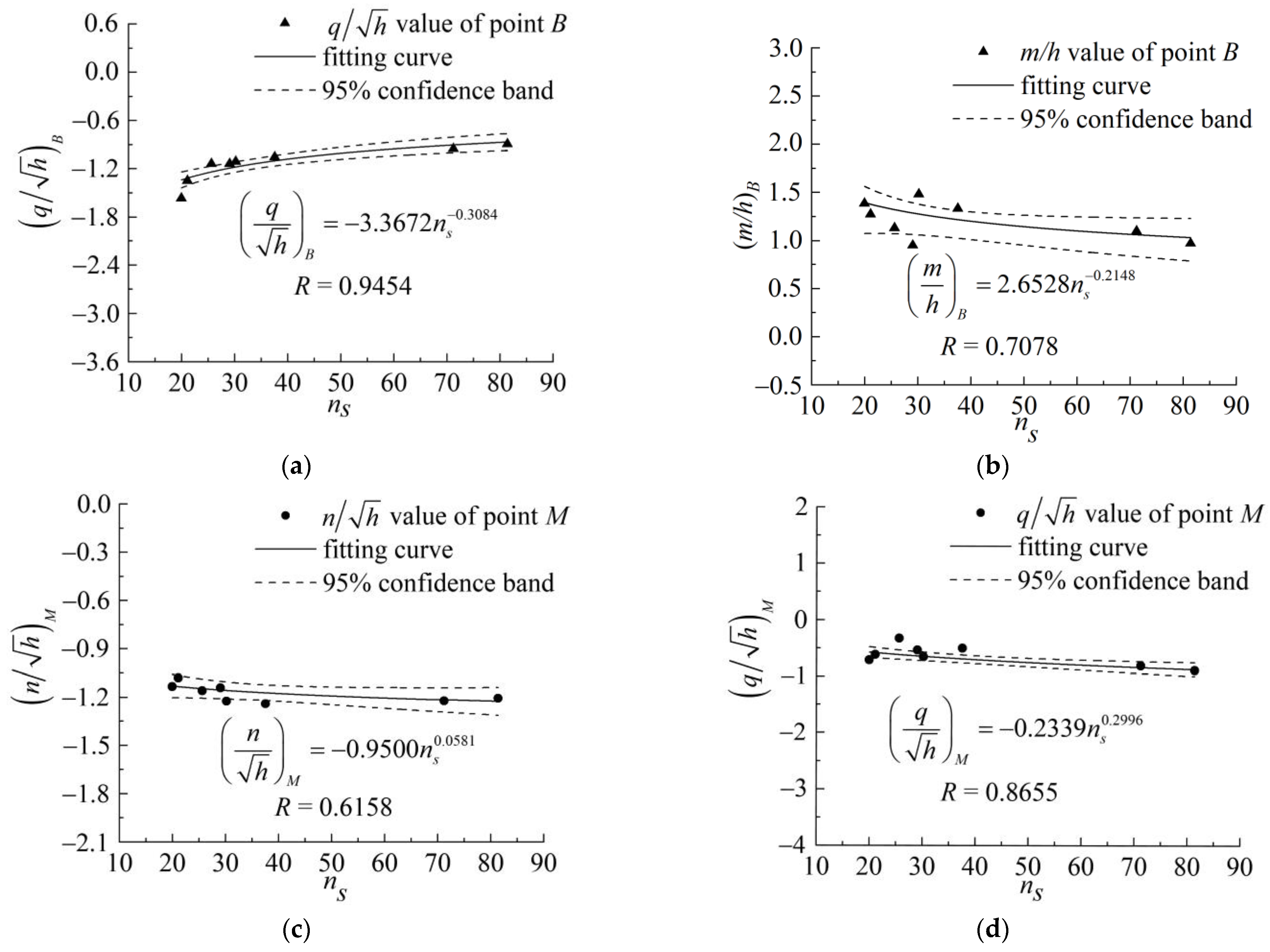
3.2.2. Characteristic Parameters of Points B and M
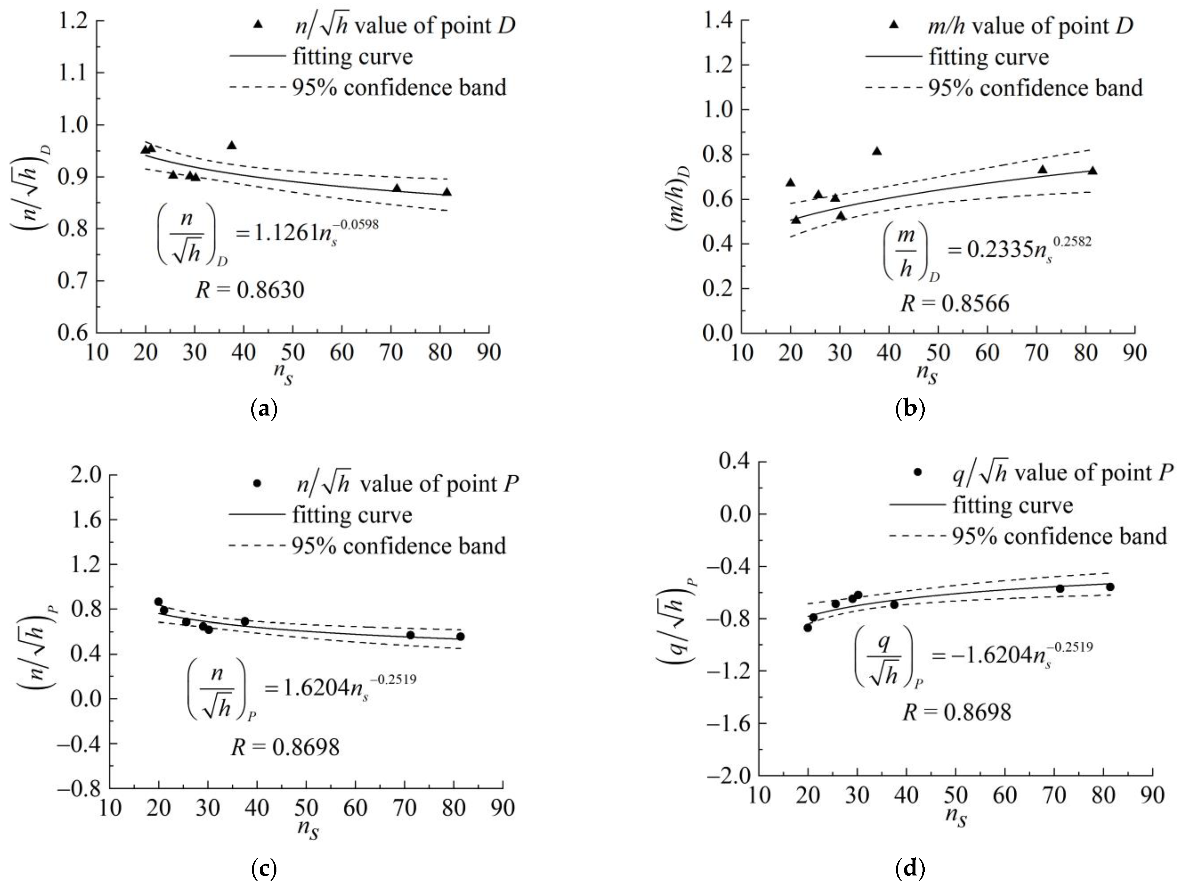
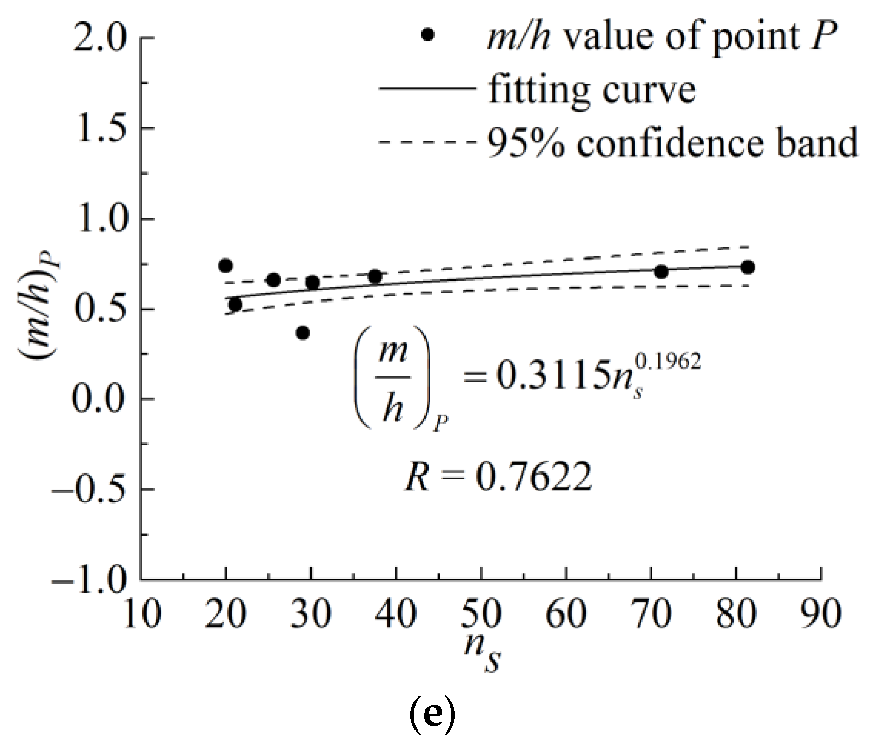
3.2.3. Characteristic Parameters of Points D and P
4. Model Verification and CPCs Prediction
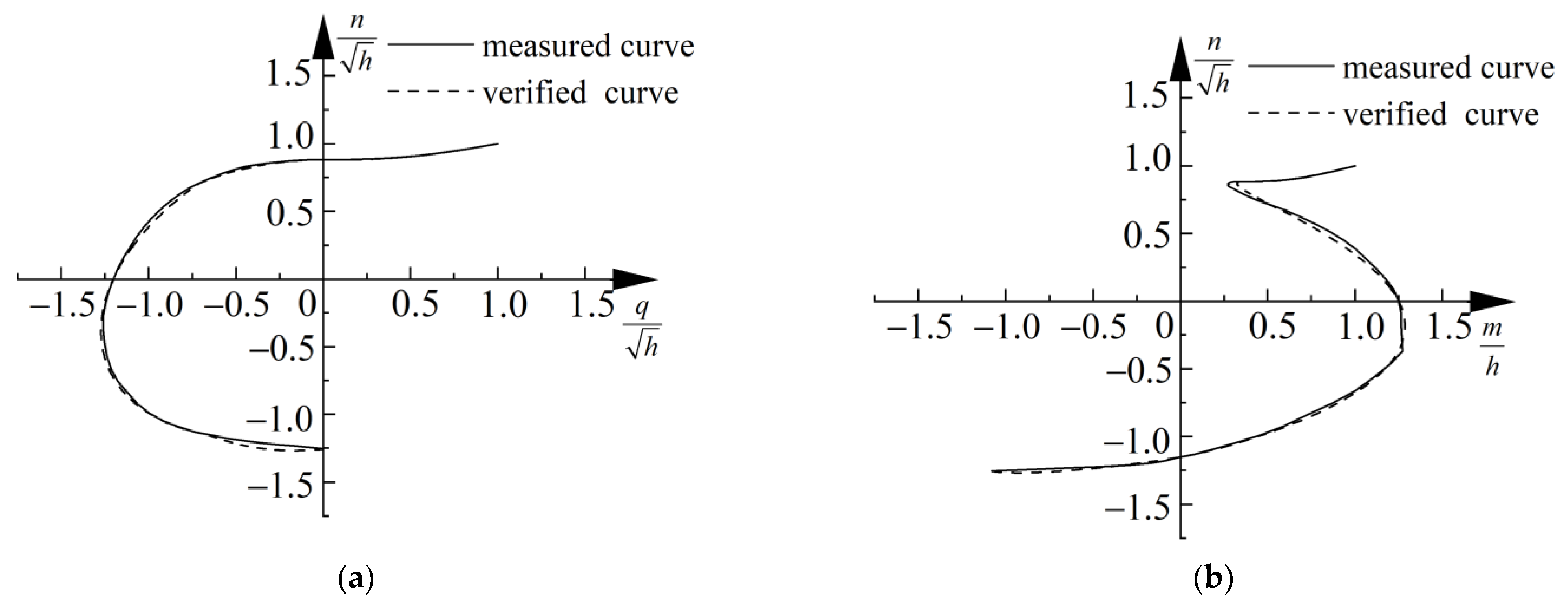
4.1. Model Verification
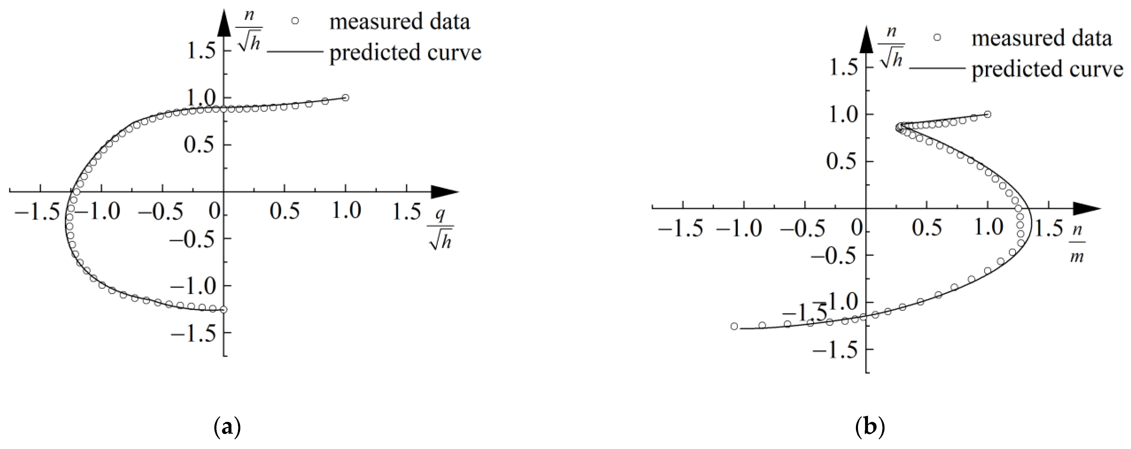
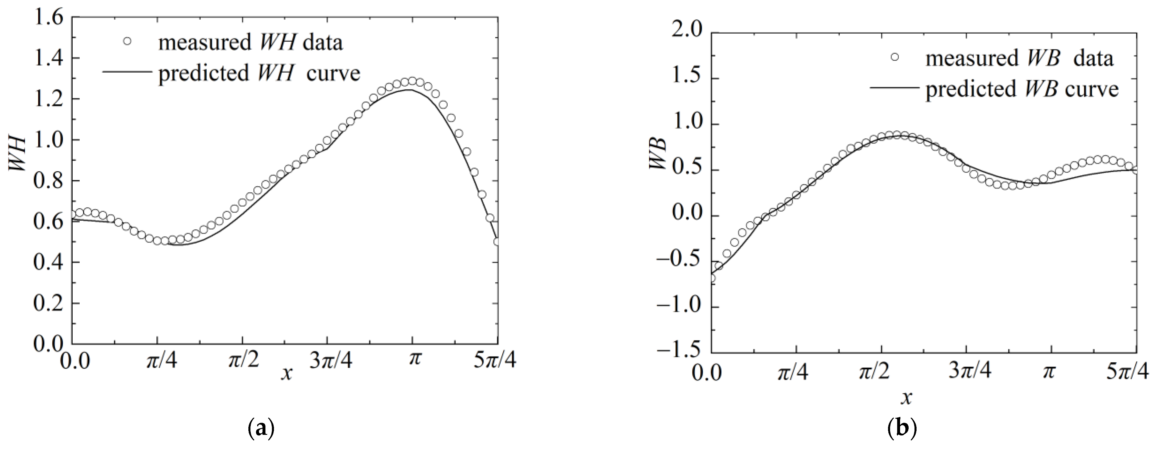
4.2. Prediction Comparison
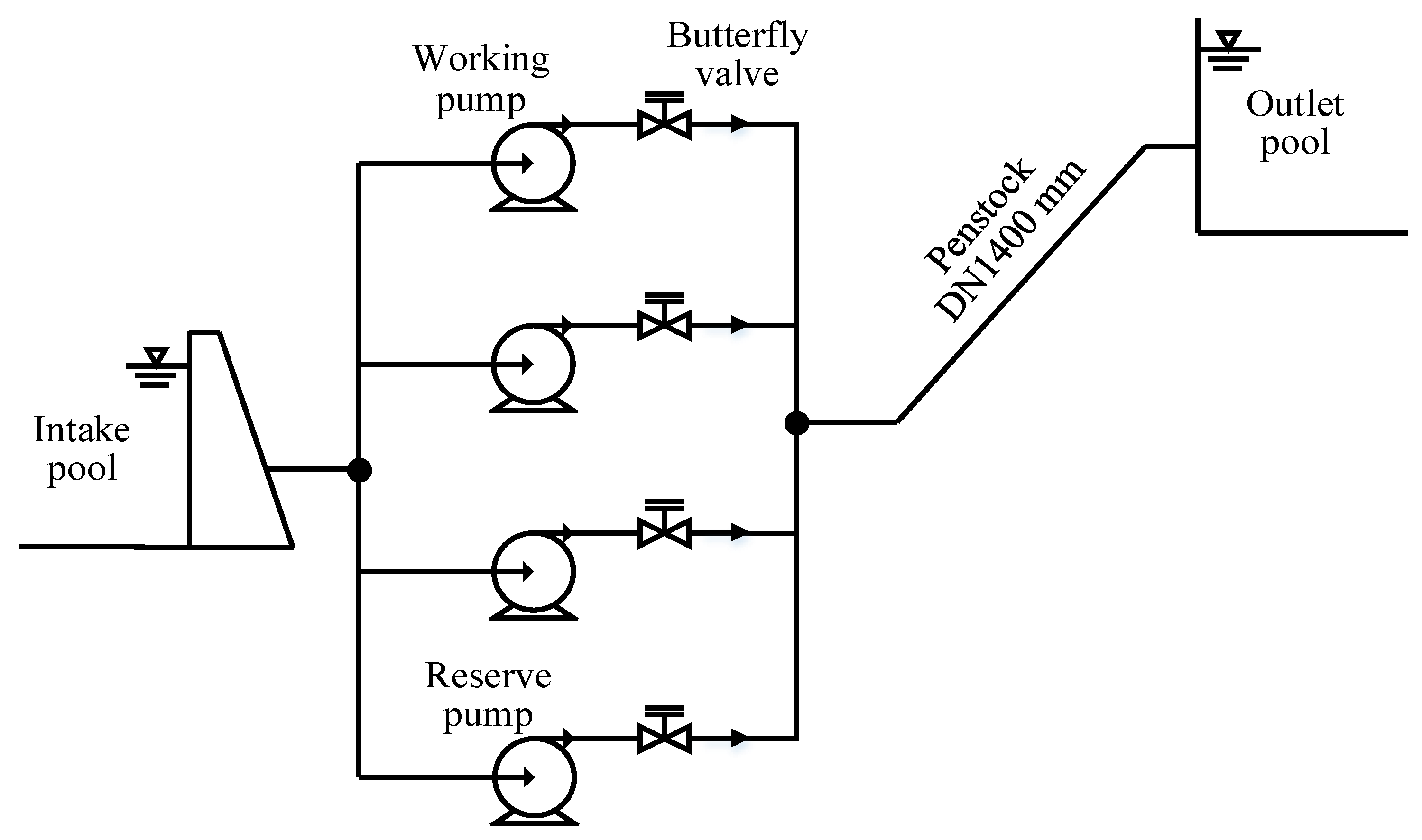
5. Case Study and Discussion
6. Conclusions
- (1)
- Under the condition that the characteristic parameters corresponding to all COPs on the and curves are known, the CPCs constructed by the mathematical model derived in this paper are in good agreement with the measured CPCs. This proves that the prediction model of the CPCs proposed in this paper is effective. When the characteristic parameters are unknown, by substituting the regression model of the characteristic parameters into the mathematical model describing the CPCs, the CPCs for a given specific speed can be predicted successfully, and the error of WH and WB values is within the acceptable range. Theoretically, the higher the statistical accuracy of characteristic parameters of COPs, the higher the prediction accuracy of the method proposed in this paper.
- (2)
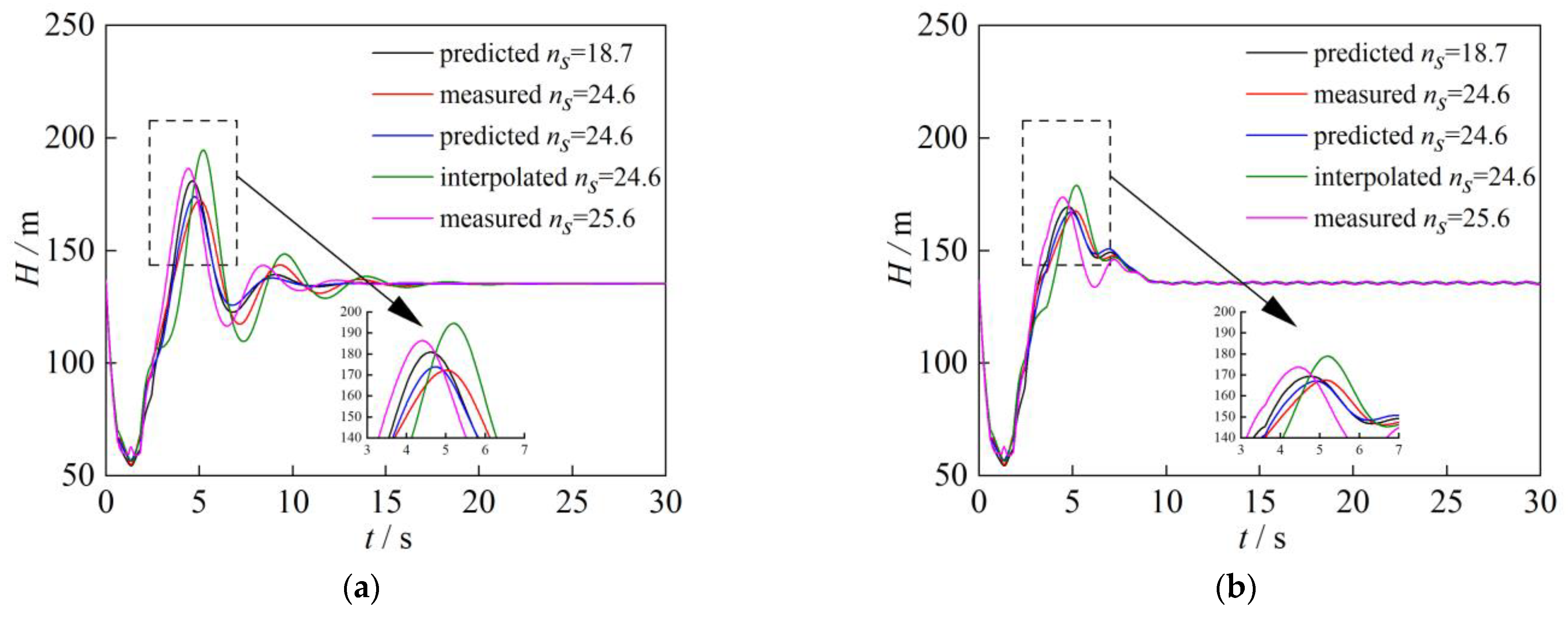
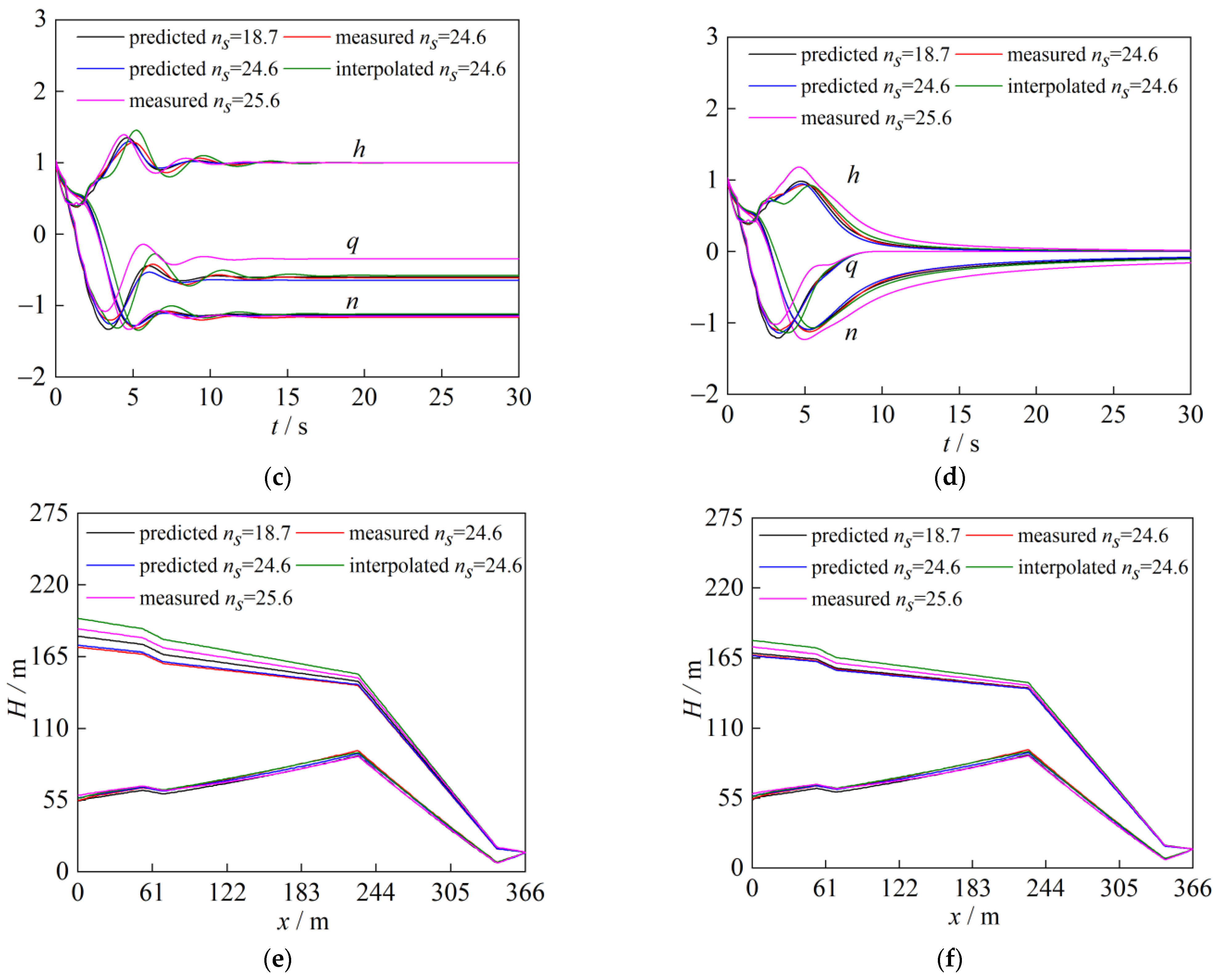
- The CPCs prediction method proposed in this paper can simulate the common transient processes of pump stations, and the error is smaller than the traditional method of using linear interpolation and using the CPCs with an approximate specific speed. The simulation accuracy of the prediction method can meet the requirements for the hydraulic transient simulation in the preliminary design, and provide important data support for the design and safe operation of the project.
Author Contributions
Funding
Institutional Review Board Statement
Informed Consent Statement
Data Availability Statement
Acknowledgments
Conflicts of Interest
Nomenclature
| CPC | complete pump characteristic |
| COP | characteristic operating point |
| M | shaft torque, N∙m |
| He | theoretical head, m |
| H | practical head, m |
| Q | discharge, m3/s |
| K | hydraulic loss coefficient |
| ω | angular velocity of rotation, rad/s |
| Vu | peripheral components of the absolute velocity, m/s |
| r | impeller radius, m |
| ρ | flow density, kg/m3 |
| g | gravitational acceleration, m/s2 |
| Vm | meridional flow velocity, m/s |
| A | section area, m2 |
| b | section width, m |
| U | peripheral velocity, m/s |
| absolute flow angle, ° | |
| relative flow angle, ° | |
| q | relative discharge |
| h | relative head |
| n | relative rotational speed |
| m | relative torque |
| N | rotational speed, rpm |
| ns | specific speed |
| WH | head characteristics of pump |
| WB | torque characteristics of pump |
| Subscripts | |
| r | rated condition |
| max. | maximum value |
| min. | maximum value |
| 1 | impeller inlet |
| 2 | impeller outlet |
References
- Wang, F.J.; Tang, X.L.; Chen, X.; Xiao, R.F.; Yao, Z.F.; Yang, W. A review on flow analysis method for pumping stations. J. Hydraul. Eng. 2018, 49, 47–61. [Google Scholar]
- Dai, C.; Dong, L.; Lin, H.; Zhao, F. A Hydraulic Performance Comparison of Centrifugal Pump Operating in Pump and Turbine Modes. J. Therm. Sci. 2020, 29, 1594–1605. [Google Scholar] [CrossRef]
- Li, D.; Fu, X.; Zuo, Z.; Wang, H.; Li, Z.; Liu, S.; Wei, X. Investigation methods for analysis of transient phenomena concerning design and operation of hydraulic-machine systems—A review. Renew. Sustain. Energy Rev. 2019, 101, 26–46. [Google Scholar] [CrossRef]
- Huang, W.; Yang, K.; Guo, X.; Ma, J.; Wang, J.; Li, J. Prediction Method for the Complete Characteristic Curves of a Francis Pump-Turbine. Water 2018, 10, 205. [Google Scholar] [CrossRef] [Green Version]
- Knapp, R.T. Complete characteristics of centrifugal pumps and their use in the prediction of transient behavior. Trans. ASME 1937, 59, 683–689. [Google Scholar]
- Huang, B.; Wu, P.; Liu, X.S.; Feng, X.D.; Yang, S.; Wu, D.Z. Four-quadrant Full Characteristic Model Test of the ACP100 Reactor Coolant Pump. Fluid Mach. 2020, 48, 8–11. [Google Scholar]
- Shukla, S.N.; Kshirsagar, J.T. Numerical Experiments on a Centrifugal Pump. In Proceedings of the ASME 2002 Joint U.S.-European Fluids Engineering Division Conference, Montreal, QC, Canada, 14–18 July 2002; pp. 709–719. [Google Scholar]
- Donsky, B. Complete Pump Characteristics and the Effects of Specific Speeds on Hydraulic Transients. J. Fluids Eng. 1961, 83, 685. [Google Scholar] [CrossRef]
- Yang, Y.S.; Dong, R.; Jing, T. Influence of Full Characteristic Curve on Pump-off Water Hammer and Its Protection. China Water Wastewater 2010, 26, 63–66. [Google Scholar]
- Marchal, M.; Flesch, G.; Suter, P. The calculation of waterhammer problems by means of the digital computer. In Proceedings of the International Symposium on Waterhammer in Pumped Storage Projects ASME, Chicago, IL, USA, 7–11 November 1965; pp. 168–180. [Google Scholar]
- Zhang, C.; Peng, T.; Zhou, J.; Ji, J.; Wang, X. An improved autoencoder and partial least squares regression-based extreme learning machine model for pump turbine characteristics. Appl. Sci. 2019, 9, 3987. [Google Scholar] [CrossRef] [Green Version]
- Izquierdo, J.; Montalvo, I.; Pérez-García, R.; Ayala-Cabrera, D. Multi-agent simulation of hydraulic transient equations in pressurized systems. J. Comput. Civ. Eng. 2016, 30, 04015071. [Google Scholar] [CrossRef] [Green Version]
- Zhu, M.L.; Zhang, X.H.; Zhang, Y.H.; Wang, T. Study on prediction model of complete characteristic curves of centrifugal pumps. J. Northwest Sci-Tech Univ. Agric. For. Nat. Sci. Ed. 2006, 4, 143–146. [Google Scholar]
- Hu, X.Y.; Yu, B.; Guo, J.; Wang, S.K. Visualization for predictable model of complete characteristic curve of pump. Fluid Mach. 2012, 3, 37–39. [Google Scholar]
- Lima, G.M.; Luvizotto Júnior, E. Method to estimate complete curves of hydraulic pumps through the polymorphism of existing curves. J. Hydraul. Eng. 2017, 143, 04017017. [Google Scholar] [CrossRef]
- Wan, W.; Huang, W. Investigation on complete characteristics and hydraulic transient of centrifugal pump. J. Mech. Sci. Technol. 2011, 25, 2583–2590. [Google Scholar] [CrossRef]
- Liu, G.L.; Jiang, J.; Fu, X.Q. Predicting complete characteristics of pumps by using BP neural network. J. Wuhan Univ. Hydraul. Electr. Eng. 2000, 2, 37–39. [Google Scholar]
- Lu, W.; Li, L.G. Drawing the all-character curve of water pump on BP neural network. Ind. Control. Comput. 2001, 14, 18–20. [Google Scholar]
- Liu, Z.F. GARBF Network Method to Predict the Complete Characteristic Curve of Pump. Master’s Thesis, Chang’an University, Xi’an, China, 2011. [Google Scholar]
- Han, W.; Nan, L.; Su, M.; Chen, Y.; Li, R.; Zhang, X. Research on the prediction method of centrifugal pump performance based on a double hidden layer BP neural network. Energies 2019, 12, 2709. [Google Scholar] [CrossRef] [Green Version]
- Huang, S.; Qiu, G.; Su, X.; Chen, J.; Zou, W. Performance prediction of a centrifugal pump as turbine using rotor-volute matching principle. Renew. Energy 2017, 108, 64–71. [Google Scholar] [CrossRef]
- Wu, Q.; Wang, X.; Shen, Q. Research on dynamic modeling and simulation of axial-flow pumping system based on RBF neural network. Neurocomputing 2016, 186, 200–206. [Google Scholar] [CrossRef]
- Höller, S.; Benigni, H.; Jaberg, H. Investigation of the 4-Quadrant behaviour of a mixed flow diffuser pump with CFD-methods and test rig evaluation. IOP Conf. Ser. Earth Environ. Sci. 2016, 49, 032018. [Google Scholar] [CrossRef]
- Gros, L.; Couzinet, A.; Pierrat, D.; Landry, L. Complete pump characteristics and 4-quadrant representation investigated by experimental and numerical approaches. In Proceedings of the ASME-JSME-KSME 2011 Joint Fluids Engineering Conference, Hamamatsu, Japan, 24–29 July 2011; pp. 359–368. [Google Scholar]
- Wang, L.; Li, M.; Wang, F.J.; Wang, J.B.; Yao, C.G.; Yu, Y.S. Study on three-dimensional internal characteristics method of Suter curves for double-suction centrifugal pump. J. Hydraul. Eng. 2017, 48, 113–122. [Google Scholar]
- Muttalli, R.S.; Agrawal, S.; Warudkar, H. CFD simulation of centrifugal pump impeller using ANSYS-CFX. Intern. J. Innov. Res. Sci. Eng. Technol. 2014, 3, 15553–15561. [Google Scholar] [CrossRef]
- Frosina, E.; Buono, D.; Senatore, A. A performance prediction method for pumps as turbines (PAT) using a computational fluid dynamics (CFD) modeling approach. Energies 2017, 10, 103. [Google Scholar] [CrossRef] [Green Version]
- Chang, J.S. Transients of Hydraulic Machine Installations; Higher Education Press: Beijing, China, 2005. [Google Scholar]
- Zhang, Y.L.; Zhu, Z.C.; Dou, H.S.; Cui, B.L. A Generalized Euler Equation to Predict Theoretical Head of Turbomachinery. Int. J. Rotating Mach. 2015, 42, 26–38. [Google Scholar] [CrossRef]
- El-Naggar, M.A. A one-dimensional flow analysis for the prediction of centrifugal pump performance characteristics. Int. J. Rotating Mach. 2013, 2013, 473512. [Google Scholar] [CrossRef] [Green Version]
- Olimstad, G.; Nielsen, T.; Børresen, B. Dependency on runner geometry for reversible-pump turbine characteristics in turbine mode of operation. J. Fluids Eng. 2012, 134, 121102. [Google Scholar] [CrossRef]
- Tanaka, T.; Liu, C. An Investigation on Velocity Triangle Applied to Fluid Particle at Rotating Flow Passage of Impeller Blade in Centrifugal Pump. In Proceedings of the ASME 7th Biennial Conference on Engineering Systems Design and Analysis, Manchester, UK, 19–22 July 2004; pp. 433–442. [Google Scholar]
- Nicolet, C. Hydroacoustic Modelling and Numerical Simulation of Unsteady Operation of Hydroelectric Systems. Ph.D. Thesis, École Polytechnique Fédérale de Lausanne (EPFL), Lausanne, Switzerland, 2007. [Google Scholar]
- Xu, H.Q.; Lu, L.; Tan, D.Q.; Li, T.Y. Specific speed of pump and unit parameter selection. In Proceedings of the 20th China Hydropower Equipment Symposium, Chengdu, China, 15–17 October 2015. [Google Scholar]
- Yang, K.L. Hydraulic Transients and Regulation in Power Station and Pump Station; China Water Conservancy and Hydropower Press: Beijing, China, 2000. [Google Scholar]
- Matteo, L.; Cerru, F.; Dazin, A.; Tauveron, N. Investigation of the pump, dissipation and inverse turbine operating modes using the CATHARE-3 one-dimensional rotodynamic pump model. In Proceedings of the ASME-JSME-KSME 2019 8th Joint Fluids Engineering Conference, San Francisco, CA, USA, 28 July–1 August 2019. [Google Scholar]
- Wu, D.Z.; Xu, B.J.; Li, Z.F.; Wang, L.Q. Numerical Simulation On Internal Flow Of Centrifugal Pump During Transient Operation. J. Eng. Thermophys. 2009, 781–783. [Google Scholar]
- Chang, J.S. Analysis of Whole Characteristic Curve and Their Special Condition Points in Mixed-flow Pump-turbine. J. Beijing Agric. Eng. Univ. 1995, 015, 77–83. [Google Scholar]
- Huang, W.; Kang, Q.; Li, S.S.; Zhu, Y.X.; Yan, F.; Li, J.Z. Analysis of the effect of valve characteristics on hydraulic transition process of pumping station. South-to-North Water Transf. Water Sci. Technol. 2019, 17, 6. [Google Scholar]
- Ayder, E.; Ilikan, A.N.; Sen, M.; Ozgur, C.; Kavurmacıoglu, L.; Kirkkopru, K. Experimental investigation of the complete characteristics of rotodynamic pumps. In Proceedings of the ASME 2009 Fluids Engineering Division Summer Meeting, Vail, CO, USA, 2–6 August 2009; pp. 35–40. [Google Scholar]
- Chen, N.X. Simulation and Control of Hydraulic Transients in Hydropower Projects; China Water Power Press: Beijing, China, 2005. [Google Scholar]
- Brown, R.J.; Rogers, D.C. Development of Pump Characteristics from Field Tests. J. Mech. Des. 1980, 102, 807–817. [Google Scholar] [CrossRef]
- Kittredge, C.; Princeton, N. Hydraulic transients in centrifugal pump systems. Trans. ASME 1956, 78, 1307–1321. [Google Scholar]
- Liu, G.L.; Guo, M.H. Computer simulation of universal complete pump characteristics. J. Hydraul. Eng. 1998, 8, 2–8. [Google Scholar] [CrossRef]
- Xie, A.; Li, D.H. Probability and Statistics; Tsinghua University Press: Beijing, China, 2012. [Google Scholar]
- Wylie, E.B.; Streeter, V.L. Fluid Transients; McGraw-Hill International Book Co.: New York, NY, USA, 1978. [Google Scholar]


| COPs | |||
|---|---|---|---|
| A | 0.0000 | −1.2559 | −1.0789 |
| M | −0.6526 | −1.1520 | 0.0000 |
| B | −1.2021 | 0.0000 | 1.2500 |
| P | −0.7085 | 0.7085 | 0.5221 |
| C | 0.0000 | 0.8811 | 0.3494 |
| D | 0.5000 | 0.9051 | 0.6592 |
| O | 1.0000 | 1.0000 | 1.0000 |
| Adopted CPCs | Condition One | Condition Two | ||||
|---|---|---|---|---|---|---|
| Max./Min. Head at Control Valve Outlet (m) | Max. Relative Reverse Speed | Max./Min. Head Along Pipeline (m) | Max./Min. Head at Control Valve Outlet (m) | Max. Relative Reverse Speed | Max./Min. Head Along Pipeline (m) | |
| Predicted ns = 18.7 | 180.87/54.42 | −1.29 | 180.87/6.66 | 169.33/54.42 | −1.10 | 169.33/6.64 |
| Measured ns = 24.6 | 172.26/54.95 | −1.32 | 172.26/7.54 | 167.59/54.95 | −1.12 | 167.59/7.67 |
| Predicted ns = 24.6 | 173.89/56.81 | −1.28 | 173.89/6.80 | 167.10/56.81 | −1.09 | 167.10/6.84 |
| Interpolated ns = 24.6 | 194.58/56.42 | −1.34 | 194.58/7.31 | 178.94/56.43 | −1.07 | 178.94/7.64 |
| Measured ns = 25.6 | 186.40/58.82 | −1.33 | 186.40/6.70 | 173.70/58.86 | −1.23 | 173.70/6.45 |
Publisher’s Note: MDPI stays neutral with regard to jurisdictional claims in published maps and institutional affiliations. |
© 2021 by the authors. Licensee MDPI, Basel, Switzerland. This article is an open access article distributed under the terms and conditions of the Creative Commons Attribution (CC BY) license (https://creativecommons.org/licenses/by/4.0/).
Share and Cite
Li, H.; Lin, H.; Huang, W.; Li, J.; Zeng, M.; Ma, J.; Hu, X. A New Prediction Method for the Complete Characteristic Curves of Centrifugal Pumps. Energies 2021, 14, 8580. https://doi.org/10.3390/en14248580
Li H, Lin H, Huang W, Li J, Zeng M, Ma J, Hu X. A New Prediction Method for the Complete Characteristic Curves of Centrifugal Pumps. Energies. 2021; 14(24):8580. https://doi.org/10.3390/en14248580
Chicago/Turabian StyleLi, Huokun, Hongkang Lin, Wei Huang, Jiazhen Li, Min Zeng, Jiming Ma, and Xin Hu. 2021. "A New Prediction Method for the Complete Characteristic Curves of Centrifugal Pumps" Energies 14, no. 24: 8580. https://doi.org/10.3390/en14248580