Improving Thermoeconomic and Environmental Performance of District Heating via Demand Pooling and Upscaling

Abstract

This study evaluates the effects of pooling heat demands in a district for the purpose of upscaling heat production units by means of energy, exergy, economic, exergoeconomic, and environmental indicators, as well as the sensitivity to investment and fuel costs. The following production systems to satisfy the heat demands (domestic hot water production and space heating) of a mixed district composed of office (80%), residential (15%), and commercial (5%) buildings are considered: gas- and biomass-fired boilers, electric boilers and heat pumps (grid-powered or photovoltaic -powered), and solar thermal collectors. For comparison, three system sizing approaches are examined: at building scale, at sector scale (residential, office, and commerce), or at district scale. For the configurations studied, the upscaling benefits were up to 5% higher efficiency (energy and exergy), there was lower levelized cost of heat for all systems (between 20% and 54%), up to 55% lower exergy destruction costs, and up to 5% greater CO₂ mitigations. In conclusion, upscaling and demand pooling tend to improve specific efficiencies, reduce specific costs, reduce total investment through the peak power sizing method, and mitigate temporal mismatch in solar-driven systems. Possible drawbacks are additional heat losses due to the distribution network and reduced performance in heat pumps due to the higher temperatures required. Nevertheless, the advantages outweigh the drawbacks in most cases.

1. Introduction

Renewable energy sources are emerging as an attractive alternative to fossil fuels owing to better availability and fewer environmental implications. Global CO₂ emissions have increased considerably since 1900, with a rise of approximately 90% from 1970 to 2011, wherein the combustion of fossil fuels and industrial processes accounted for 78% of the total greenhouse gas emissions [1]. As a result, several countries have established objectives to reduce greenhouse gas emissions and have introduced policies to promote the implementation of low-carbon technologies such as renewable energy [2,3,4]. Zappa et al. [5] examined the feasibility of a 100% renewable energy-based European power system and compared the economic gains with respect to a non-renewable energy-driven system. The results from their study indicate that a 100% renewable European power system could potentially provide similar system sufficiency to the present power system, even when utilizing the European sources alone. However, the total annual cost of a 100% renewable system was found to be at least 30% higher than for a system including nuclear technologies or carbon fuels. In France, space heating and water heating accounted for a major share (about 77%) of the energy consumption in the building sector in 2017 [6]. Therefore, the energy practices and strategies pertaining to space heating and hot water production play a significant role in controlling environmental impacts.

District-scale heating systems for space heating and hot water production may lead to better productivity of units, reduced carbon emissions, and lower lifetime costs when compared to decentralized heating systems [7]. Ghafghazi et al. [8] examined four energy sources, namely, natural gas, biomass, sewer heat, and geothermal heat, for hot water production in a newly developed district in Vancouver, Canada. These energy sources were ranked based on their cost, greenhouse gas emissions, particulate matter emission, maturity of technology, whether the source is locally available or not, and traffic burden from using the source. They found that biomass and sewer heat were the most promising solutions, although the final selection would depend on the scenario. Wang et al. [9] performed modeling and optimization of a combined heating and power-based district heating system including renewable energy sources (solar thermal power plant) and thermal energy storage. A comparison of distributed and centralized solar collectors assisting an existing district heating system [10] revealed cost savings between 7% and 21% for centralized collector systems. Renaldi and Friedrich [11] investigated the installation of a solar district heating system (the Drake Landing Solar Community in Okotoks, Canada) at two locations in the UK. The district heating system studied was found to have a higher levelized cost of energy, although it had an improved solar fraction, compared to the typical systems in Europe. Alsagri et al. [12] concluded that district heating systems with decentralized heat storage and triple pipes in the distribution and service pipeline network exhibit a better thermodynamic and economic performance when compared with conventional district heating systems. Balić et al. [13] examined the operational strategy of a combined heating and power plant coupled with a district heating system. The district heating system was identified as a possible dynamic storage, with thermal energy stored in the pipeline network, for excess energy generated by combined heating and power plants. Jonynas et al. [14] provided a comprehensive review of the use of renewable energy in district heating systems in Lithuania. Biomass and biofuels were reported to be one of the most important renewable energy sources for district heating in Lithuania.

There are several studies in the literature that demonstrate and justify the relevance of exergy analysis [15] and exergoeconomic analysis [16] at district scales. On the basis of the analysis criteria, it is possible to suggest system designs and architectures that are distinct from those proposed by other classic indicators. Our previous investigations included 5E analyses of heat production systems for one dwelling [17] and preliminary explorations of larger-scale systems [18].

The current state of the art includes some studies that compare centralized and decentralized solutions, thus addressing the notion of upscaling, at least implicitly. However, few studies use second-law or environmental indicators to evaluate the effects of upscaling. Our study contributes to this research gap by including exergy, exergy destruction costs, and carbon dioxide emissions in the assessment. In addition, the authors assess whether upscaling alters the economic sensitivity of the systems. More precisely, the sensitivity of the levelized cost of energy (LCOE) and of the costs of exergy destruction was scrutinized.

In the present study, different systems (based on both renewable and non-renewable energy sources) for heating needs are investigated, including space heating (SH) and domestic hot water (DHW) production, and compared at three scales: building, sector, and district. The heat production systems examined include biomass boilers, natural gas boilers, electric boilers driven by grid or photovoltaic (PV) panels, heat pumps (HP) driven by grid or PV panels, and solar thermal (ST) panels. The heat production systems were evaluated in terms of energy, exergy, economic, environmental, and exergoeconomic indicators for the Cassine district in Chambéry (France). Further, the performance of the systems was assessed according to the different sectors (residential, office, and commercial) in the district. The results from this study generate several discussions and insights into the implementation of different district heating technologies and the future scope of research.

2. Materials and Methods

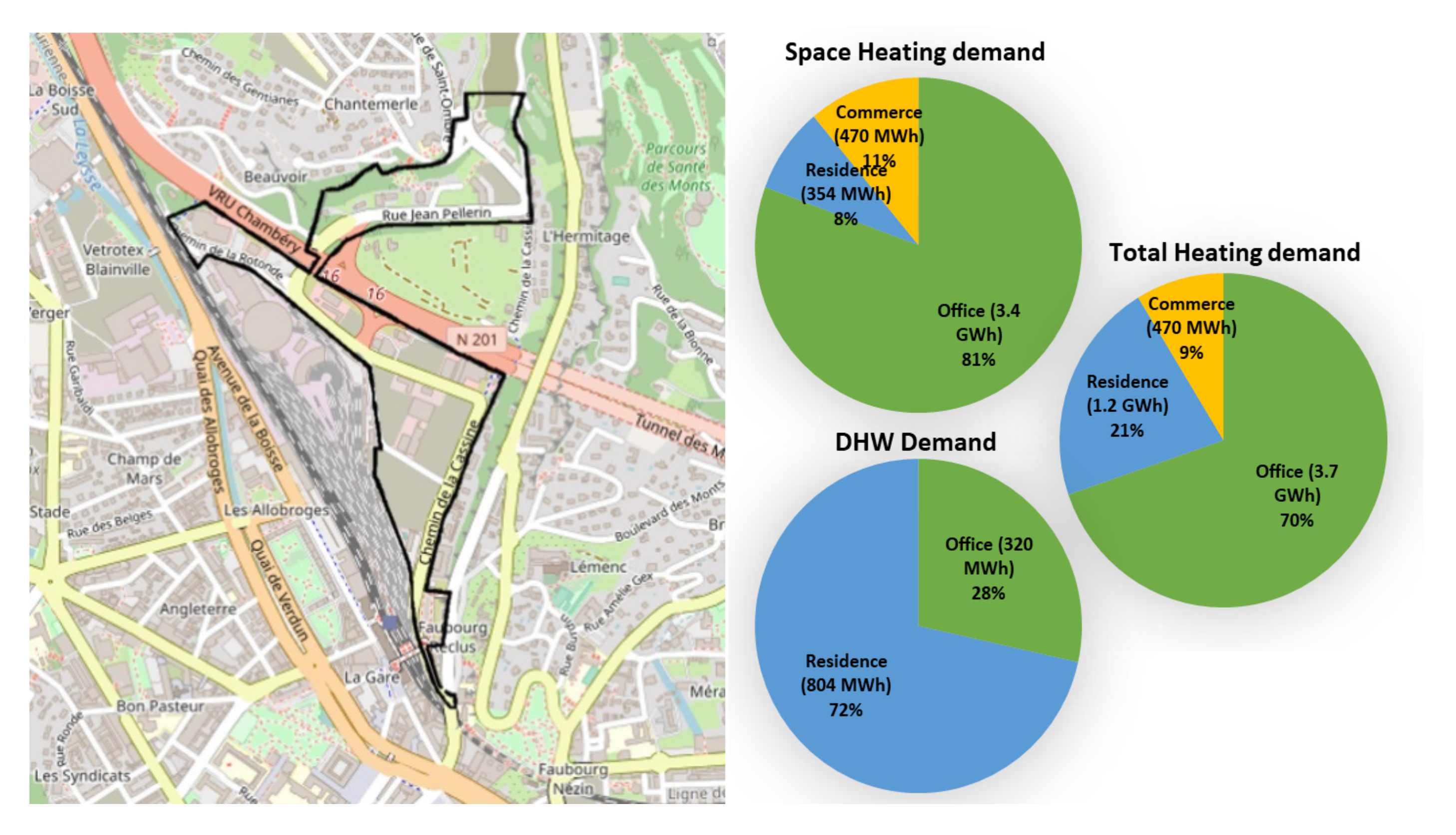
In order to evaluate the effects of pooling heat demands in the mixed district of the Cassine, France, three system sizing approaches for several heat production systems are examined: at building scale, at sector scale (residential, office, and commerce), or at district scale. The case study is first detailed, followed by the considered heat production systems’ description. Next, the energy, exergy, and cash flow balances are set, introducing the energy, exergy, economic, exergoeconomic, and environmental indicators assessment.

2.1. Case Study

The Cassine district in Chambéry, France (Figure 1), was chosen for the investigation of different heat production systems to meet the needs of space heating (source at 35 °C) and hot water production (at 65 °C). The Cassine district is primarily an office district (about 80% offices), with office buildings occupying a total surface area of 100,000 m² [19]. The collective residential and commercial sectors are spread over surface areas of 17,580 m² and 5200 m², respectively. The surface areas of the different types of buildings (belonging to each sector) are listed in

Table A1. Annual consumption of buildings constructed after 2012 in H1 zone (Chambéry, France).

Sector	Building Surface Area	Total Surface Area [m2]	Space Heating Consumption [kWh/m2]	DHW Consumption [kWh/m2]
Residential	70 m2 or less	8064	20.0	28.0
	Between 70–100 m2	5757	19.9	16.1
	Between 100–150 m2	1584	20.8	11.1
	Greater than 150 m2	2173	20.6	6.9
Office	1000 m2 or less	0 m2	35.7	3.2
	Between 1000–5000 m2	31,000 m2	34.9	3.2
	Greater than 5000 m2	69,000 m2	34.1	3.2
Commerce	125 m2 or less	2600 m2	82.5	–
	Greater than 125 m2	2600 m2	98.3

(Appendix A).

The annual and hourly space heating profiles for the collective residential housing were estimated from the PHEBUS studies [20,21], respectively. The annual space heating profiles for tertiary buildings (office and commerce) were evaluated using the CEREN publications [21,22,23]. The hourly space heating demands were then evaluated using the tool proposed in [24] for offices, whereas the ARENE/ADEME report [25] was used for the commercial buildings. The total annual space heating demands for offices, residences, and commercial buildings in the Cassine district were estimated as 3.4 GWh, 354 MWh, and 470 MWh, respectively (Figure 1).

The domestic hot water (DHW) profiles for the collective residential sector were obtained using the ADEME report [26] with an average of 2.2 persons per household in France [27]. The annual DHW demand for office buildings was evaluated considering an average DHW consumption of 2 L per day per employee [28], an average surface area per employee of 12 m², and 20% additional surface for the bathroom, office equipment, etc. [20] with the temperature difference set at 55 °C (i.e., 65–10 °C). Therefore, the average annual DHW demand per employee was calculated to be 46.6 kWh/employee, and the average annual DHW demand per square meter was estimated as 3.2 kWh/m² for office buildings. In order to obtain the hourly DHW profiles for offices, the annual DHW demand was assumed to be equally distributed between office working hours from 08:00 h to 18:00 h, while the hourly DHW demands from 19:00 h to 07:00 h were assumed to be null. The annual DHW needs for offices and collective residential sectors were evaluated to be 320 MWh and 804 MWh, respectively (Figure 1).

The DHW demand profiles for the commercial sector vary significantly from one type of commerce to another. Thus, the DHW demand of the commercial buildings was not considered in this study.

The total annual heating demands calculated for the buildings constructed after 2012, in Chambéry (i.e., H1 zone as per the RT2012 legislation), are summarized in Table A1 (Appendix A) [20,21,22,23,26,27,28,29]. The annual space heating and DHW demands were then computed for each sector in the Cassine district (Chambéry) from

Table 1. Production systems considered in this study and their main units.

System	Scale of Sizing	Energy Unit(s)	Backup Unit(s)
GBOIL	Building	Gas boiler (GBOIL)	Not needed
	Sector or District	GBOIL + DHN
BBOIL	Building	Biomass boiler (BBOIL)	Not needed
	Sector or District	BBOIL + 80 °C/60 °C network (DHN)
Grid + EBOIL	Building	Grid-driven electric boiler (EBOIL)	Not needed
	Sector or District	EBOIL + DHN
PV + EBOIL	Building	Photovoltaic panels (PV)	Grid + EBOIL
	Sector or District	PV + EBOIL + DHN
ST	Building	Solar thermal collectors (ST)	Grid + EBOIL
	Sector or District	ST + DHN
Grid + HP	Building	Air-source heat pump (ASHP)	Not needed
	Sector or District	Geothermal HP (GHP) + DHN
PV + HP	Building	ASHP (PV-driven)	Grid + HP
	Sector or District	GHP (PV-driven) + DHN

based on the type of building (residential, office, or commercial) and the surface area of the buildings. Figure 1 also illustrates the share of each sector in the annual heating demands. The office sector dominates the space heating demand, as expected. This is the result of the specific mix of buildings in the Cassine district, which comprises primarily offices. In addition, the space heating demand of the commercial sector is higher than the residential sector. Even though the residential sector covers a larger surface area in the district, the consumption of commercial buildings is substantially higher. Moreover, in the case of DHW consumption, the residential sector surpasses the offices, as expected. Furthermore, it is worth noting that the total heating demand of the commercial sector does not include DHW demand and, therefore, corresponds to the lowest share. The total heating demand is the highest for office buildings since the relative magnitude of space heating demand is considerably higher than the DHW demand, thereby influencing the total demand to a greater extent.

Thereafter, the hourly demand profiles were determined using the coefficients indicating the percentage distribution of the annual demand depending on the month, day of the week, and hour of the day. These coefficients were obtained for each type of building based on [21,24,25,26] and on the assumption of uniform DHW consumption (only between 08:00 h and 18:00 h) in office buildings, as stated earlier. The percentage distribution coefficients for office, residential, and commercial buildings for space heating and DHW demands are given in

Table A2. Percentage distribution coefficients for space heating and domestic hot water consumption in residential (R), office (O), and commerce (C) sectors.

Hour	R				O		C	Day	R		O		C
	SH	DHW			SH	DHW	SH		SH	DHW	SH	DHW	SH
		Sat	Sun	Others
00:00	2.2%	1.8%	1.5%	1.7%	2.8%	0%	2.8%	Mon	13.6%	13.7%	17.4%	20%	18.5%
01:00	2.2%	1.0%	1.0%	0.9%	2.8%	0%	3.4%	Tue	13.6%	13.4%	17.5%	20%	16.0%
02:00	2.5%	0.6%	0.6%	0.5%	2.9%	0%	3.1%	Wed	13.6%	14.0%	17.3%	20%	15.0%
03:00	2.5%	0.5%	0.4%	0.4%	3.0%	0%	3.2%	Thu	13.6%	13.7%	17.5%	20%	15.3%
04:00	2.8%	0.5%	0.4%	0.7%	3.1%	0%	3.0%	Fri	13.6%	13.9%	16.0%	20%	15.0%
05:00	4.0%	0.8%	0.6%	1.4%	4.8%	0%	3.2%	Sat	16.0%	14.0%	7.3%	0%	13.2%
06:00	4.9%	1.3%	0.8%	2.8%	8.1%	0%	3.3%	Sun	16.0%	17.3%	7.0%	0%	7.0%
07:00	5.0%	2.6%	1.3%	3.9%	7.4%	0%	3.2%
08:00	5.0%	4.1%	2.6%	4.3%	6.5%	9.09%	3.5%
09:00	5.1%	5.9%	4.5%	5.0%	5.5%	9.09%	5.7%
10:00	5.0%	6.4%	6.0%	5.2%	5.1%	9.09%	7.2%	Month	R		O		C
11:00	4.8%	7.1%	7.1%	5.7%	4.5%	9.09%	6.4%		SH	DHW	SH	DHW	SH
12:00	4.5%	7.5%	7.6%	7.0%	4.5%	9.09%	6.4%	Jan	15.5%	8.9%	15.0%	8.33%	15.3%
13:00	4.4%	7.5%	7.4%	6.4%	4.2%	9.09%	6.0%	Feb	14.0%	8.8%	14.0%	8.33%	14.0%
14:00	4.3%	6.6%	6.0%	4.5%	4.0%	9.09%	5.7%	Mar	12.5%	8.9%	12.2%	8.33%	12.3%
15:00	4.2%	5.0%	5.3%	4.0%	4.0%	9.09%	5.1%	Apr	9.5%	8.4%	9.0%	8.33%	8.5%
16:00	4.2%	4.9%	5.0%	4.7%	3.9%	9.09%	4.6%	May	5.0%	8.4%	5.0%	8.33%	5.1%
17:00	4.3%	5.5%	6.0%	5.9%	3.6%	9.09%	4.8%	Jun	2.5%	8.1%	3.0%	8.33%	3.0%
18:00	4.6%	6.2%	7.6%	6.9%	3.7%	9.09%	5.1%	Jul	1.5%	7.2%	2.0%	8.33%	2.0%
19:00	4.8%	6.4%	8.2%	7.7%	4.2%	0%	4.3%	Aug	1.5%	6.5%	2.0%	8.33%	2.0%
20:00	4.8%	6.2%	7.8%	7.6%	3.5%	0%	3.0%	Sep	3.5%	8.0%	3.5%	8.33%	3.5%
21:00	5.0%	4.9%	5.7%	5.7%	2.5%	0%	2.5%	Oct	7.0%	8.6%	7.5%	8.33%	7.5%
22:00	4.8%	3.9%	4.0%	4.1%	2.7%	0%	2.5%	Nov	12.5%	9.0%	12.0%	8.33%	12.0%
23:00	4.3%	2.8%	2.6%	3.0%	2.7%	0%	2.4%	Dec	15.0%	9.2%	14.8%	8.33%	14.8%

(Appendix A).

To obtain the hourly DHW profiles for offices, the annual DHW demand was assumed to be equally distributed during office working hours from 08:00 h to 18:00 h, while the hourly DHW demands from 19:00 h to 07:00 h were assumed to be null. The percentage of hourly consumption over the year could, therefore, be evaluated by multiplying the distribution coefficients for hour, day, and month in order to determine the hourly load profiles. For example, the hourly residential space heating consumption at 08:00 h on Friday in January was calculated as 0.11% (5.0% × 13.6% × 15.5%) of the annual demand.

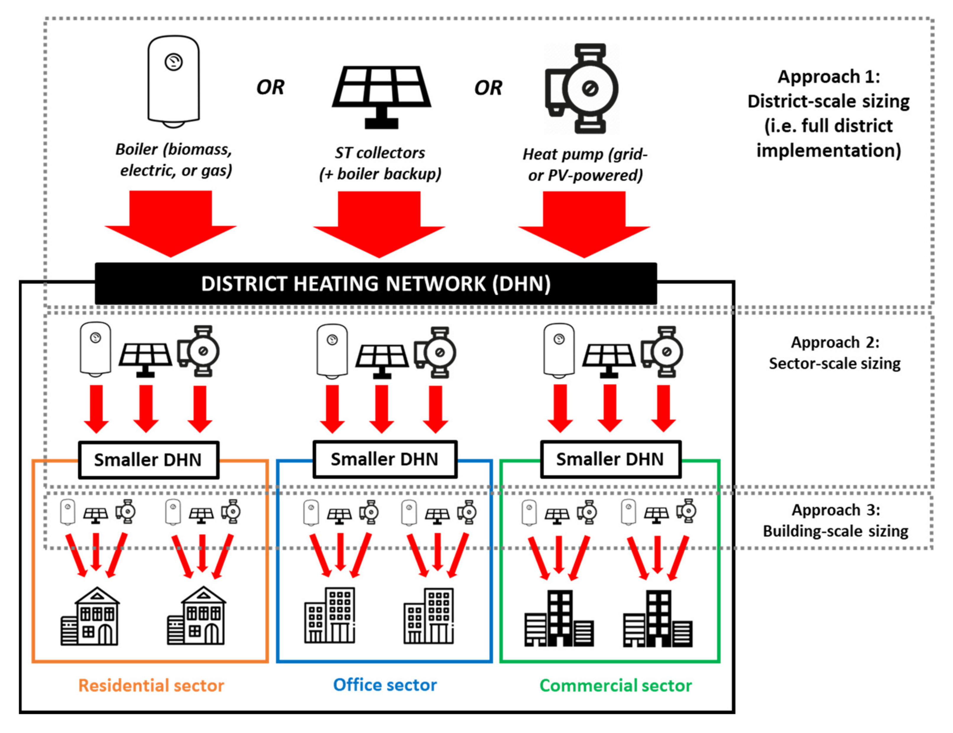
2.2. Systems for Heat Production

This study investigated several types of units that are commonly used for heating, both at building scale and at district scale, as represented in Figure 2. Seven unique solutions were considered, encompassing both renewable and non-renewable sources. Table 1 shows these solutions, the units included, and the backup system, whenever needed. Building scale means that one unit was sized for every building. Sector scale means that a small district heating network (DHN) was sized in order to cover the demands of an entire typology of buildings, i.e., office, residential, or commercial. Sector scale assumes that the same types of buildings are geographically close to each other. District scale means that needs for the whole district are aggregated into one common DHN.

Thermal storage units were considered for solar-driven systems only. This relates to ST collectors, PV-powered boilers, and PV-powered heat pumps. The same scaling approaches of production units were applied to storage units, i.e., one per building, per sector, or for the whole district. As sizing rule, the storage capacity was assumed to be equal to 60% of the highest daily heat demand for the target profile (i.e., per building, per sector, or for the district). In all cases, the day of the year with the highest demand was in December or in January. Optimizations of the storage size were considered to be out of the scope of this study.

The inlet temperature of the heating network was assumed to be 80 °C in all scenarios, which corresponds to a 3rd generation district heating system [30]. Heat losses of 5% of the total energy were assumed for the network, in all scenarios [31]. Essentially, a backup was necessary whenever the main source was subject to temporal mismatch, as is the case with any solar-driven solution. The peak power sizing method was applied to all production units. Note that peak powers are different in each scenario, due to the different scales. This has consequences for specific investment costs, which are detailed in the next subsection.

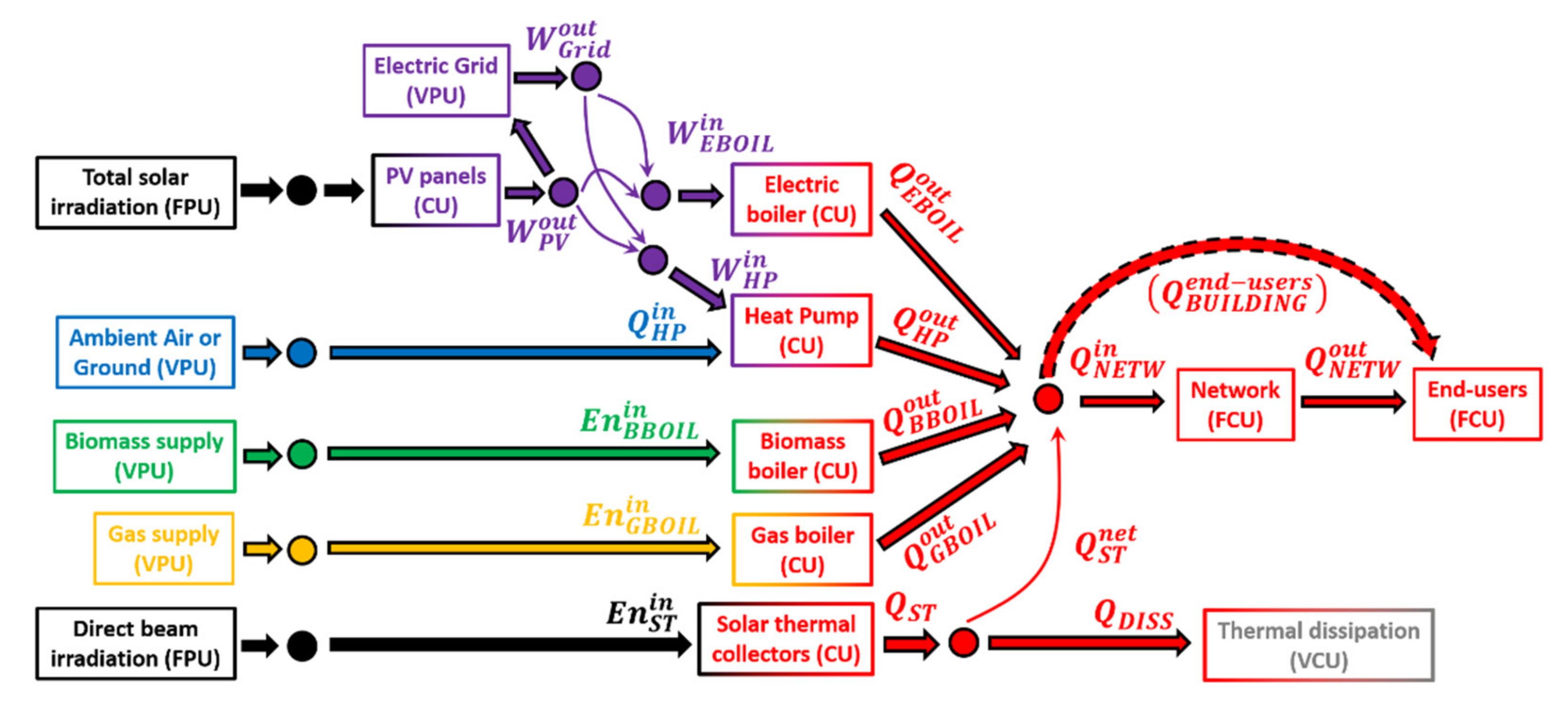
2.3. Simulation Model

The analysis was based on yearly simulations at an hourly time step, assuming a pseudo-steady state at each time step. A nodal model was used (Figure A1, Appendix A), where each node represents either an energy unit or an intersection of energy flows. In each scenario, input parameters were adjusted to ensure that only the targeted production system was used.

Simulations were solved by means of the optimization models generation as linear program for energy system (OMEGAlpes) tool [32,33,34], i.e., an open-source decision support tool conceived to simulate management of energy units. Using mixed-integer linear programming, this tool arranges the use of available energy sources and units to meet users’ objectives. Then, users may apply these results to support their investment decisions. Thus, OMEGAlpes is an optimizer of energy management that supports optimization of equipment size.

A series of assumptions in this study allow linearizing the optimization problem. First, pseudo-steady state was assumed at each time step. Second, equipment off-design was not considered in this study, as temperature levels and equipment performance were assumed constant throughout the year, based on yearly average values. Temperatures were input parameters, so there was no non-linearity of exergy due to temperature variation. Last, the sizes of units were not optimization parameters, but input parameters with fixed values. In each scenario, unit sizes were adjusted to the users’ energy needs, disregarding partial load operation. Consequently, there was no non-linearity on investment costs, as for the operational costs of any downstream energy flow because specific costs of all fuels were assumed constant.

The hypothesis of pseudo-steady state enabled step-by-step balances, understanding energy flows as instantaneous power flows. Through this hypothesis, energy, exergy, and cost flow balances were applied for each node, at every time step. The general energy balance accounts for all inlets/outlets of heat, electric power, or other forms of energy (chemical potential, solar irradiation), including energy losses:

$$\sum \dot{E}{n}^{in}=\sum \dot{E}{n}^{out}+\Delta U$$

(1)

The accumulation term applies to the thermal storage unit only.

Similarly, the general exergy balance accounts for all exergy inlets, outlets, and destructions within the unit:

$$\sum \dot{E}{x}^{in}=\sum \dot{E}{x}^{out}+\dot{E}{x}^D+\Delta U^{ex}$$

(2)

The exergy accumulation term applies to the thermal storage unit only.

Unit-by-unit energy and exergy balances as well as the auxiliary equations are given in

Table A3. Specific formulation of unit-by-unit energy and exergy balances and auxiliary equations.

Unit	Energy and Exergy Balances	Auxiliary Equations
GBOIL	$\dot{E}{n}_{GBOIL}^{in}={\dot{Q}}_{GBOIL}^{out}+\dot{E}{n}_{GBOIL}^L$	${\dot{Q}}_{GBOIL}^{out}={\eta }_{GBOIL}·\dot{E}{n}_{GBOIL}^{in}$
	$\dot{E}{x}_{GBOIL}^{in}=\dot{E}{x}_{GBOIL}^{Q,out}+\dot{E}{x}_{GBOIL}^L+\dot{E}{x}_{GBOIL}^D$	$\dot{E}{x}_{GBOIL}^{Q,out}={\dot{Q}}_{GBOIL}^{out}·\left(1-T_0/T_{GBOIL}^{out}\right)$
BBOIL	$\dot{E}{n}_{BBOIL}^{in}={\dot{Q}}_{BBOIL}^{out}+\dot{E}{n}_{BBOIL}^L$	${\dot{Q}}_{BBOIL}^{out}={\eta }_{BBOIL}·\dot{E}{n}_{BBOIL}^{in}$
	$\dot{E}{x}_{BBOIL}^{in}=\dot{E}{x}_{BBOIL}^{out}+\dot{E}{x}_{BBOIL}^L+\dot{E}{x}_{BBOIL}^D$	$\dot{E}{x}_{BBOIL}^{Q,out}={\dot{Q}}_{BBOIL}^{out}·\left(1-T_0/T_{BBOIL}^{out}\right)$
Grid	$\dot{E}{n}_{Grid}^{in}={\dot{W}}_{Grid}^{out}+\dot{E}{n}_{Grid}^L$	${\dot{W}}_{Grid}^{out}={\eta }_{Grid}·\dot{E}{n}_{Grid}^{in}$
	$\dot{E}{x}_{Grid}^{in}={\dot{W}}_{Grid}^{out}+\dot{E}{x}_{Grid}^L+\dot{E}{x}_{Grid}^D$	$\dot{E}{x}_{Grid}^{in}=\dot{E}{n}_{Grid}^{in}; \dot{E}{x}_{Grid}^L=\dot{E}{n}_{Grid}^L$
EBOIL	${\dot{W}}_{EBOIL}^{in}={\dot{Q}}_{EBOIL}^{out}$	${\dot{W}}_{EBOIL}^{in}={\dot{W}}_{Grid}^{out,EBOIL}+{\dot{W}}_{PV}^{out,EBOIL}$
	$\dot{E}{x}_{EBOIL}^{in}=\dot{E}{x}_{EBOIL}^{Q,out}+\dot{E}{x}_{EBOIL}^D$	$\dot{E}{x}_{EBOIL}^{in}={\dot{W}}_{EBOIL}^{in}$; $\dot{E}{x}_{EBOIL}^{Q,out}={\dot{Q}}_{EBOIL}^{out}·\left(1-T_0/T_{EBOIL}^{out}\right)$
ST	$\dot{E}{n}_{ST}^{in}={\dot{Q}}_{ST}^{out}+\dot{E}{n}_{ST}^L$	${\dot{Q}}_{ST}^{out}={\eta }_{ST}·\dot{E}{n}_{ST}^{in}$
	$\dot{E}{x}_{ST}^{in}=\dot{E}{x}_{ST}^{Q,out}+\dot{E}{x}_{ST}^L+\dot{E}{x}_{ST}^D$	$\dot{E}{x}_{ST}^{Q,out}={\dot{Q}}_{ST}^{out}·\left(1-T_0/T_{ST}^{out}\right)$; $\dot{E}{x}_{ST}^{in}=\dot{E}{n}_{ST}^{in}·\left(1-T_0/T_s\right)$
HP	${\dot{Q}}_{HP}^{in}+{\dot{W}}_{HP}^{in}={\dot{Q}}_{HP}^{out}$	${\dot{W}}_{HP}^{in}={\dot{W}}_{Grid}^{out,HP}+{\dot{W}}_{PV}^{out,HP}$; $CO{P}_{HP}={\dot{Q}}_{HP}^{out}/{\dot{W}}_{HP}^{in}$
	$\dot{E}{x}_{HP}^{Q,in}+{\dot{W}}_{HP}^{in}=\dot{E}{x}_{HP}^{Q,out}$	$\dot{E}{x}_{HP}^{Q,out}={\dot{Q}}_{HP}^{out}·\left(1-T_0/T_{HP}^{out}\right)$
PV	$\dot{E}{n}_{PV}^{in}={\dot{W}}_{PV}^{out}+\dot{E}{n}_{PV}^L$	${\dot{W}}_{PV}^{out}={\eta }_{PV}·\dot{E}{n}_{PV}^{in}$
	$\dot{E}{x}_{PV}^{in}={\dot{W}}_{PV}^{out}+\dot{E}{x}_{PV}^L$	$\dot{E}{x}_{PV}^{in}=\dot{E}{n}_{PV}^{in}·\left(1-T_0/T_S\right)$
DHN	${\dot{Q}}_{\mathrm{DHN}}^{in}={\dot{Q}}_{\mathrm{DHN}}^{out}+{\dot{Q}}_{\mathrm{DHN}}^L$	${\dot{Q}}_{\mathrm{DHN}}^L={\varphi }_{\mathrm{DHN}}^L·{\dot{Q}}_{\mathrm{DHN}}^{in}$
	$\dot{E}{x}_{\mathrm{DHN}}^{Q,in}=\dot{E}{x}_{\mathrm{DHN}}^{Q,out}+\dot{E}{x}_{\mathrm{DHN}}^L+\dot{E}{x}_{\mathrm{DHN}}^D$	$\dot{E}{x}_{\mathrm{DHN}}^Q={\dot{Q}}_{\mathrm{DHN}}·\left(1-T_0/T\right)$

(Appendix A). In the case of electricity or mechanical work, energy equals exergy. With transferred heat, exergy depends on temperature (see auxiliary equations in Table A3 in Appendix A). A dead state temperature of T₀ = −11 °C was used, as this is the typical design temperature suggested by the French RT2012 legislation on building energetics in the H1 climatic zone of France [24].

The general cost flow balance accounts for monetary flows attributable to fuel consumption, capital investment recovery, operating and maintenance expenses, and product selling:

$$\sum {\dot{C}}^F+{\dot{Z}}^{CI}+{\dot{Z}}^{OM}=\sum {\dot{C}}^P$$

(3)

When formulated on an energy-specific basis, fuel and product costs become a function of inlet and useful outlet energy flows, respectively. In this study, investment amortization costs were a function of the unit’s peak power. Furthermore, operating and maintenance (OM) costs were a function of investment amortization costs, using the OM factor ${\varphi }^{OM}$. Cost flow balance is thus written as:

$$\sum c^F·\dot{E}{n}^F+z^{CI}·\wp ·CRF+{\varphi }^{OM}·{\dot{Z}}^{CI}=\sum c^P·\dot{E}{n}^P$$

(4)

The capital recovery factor (CRF) was used to estimate investment amortization requirements as a function of the effective rate of return i (assumed to be 5%) and the economic lifespan n (which depends on equipment):

$$CRF=\frac{i·{\left(1+i\right)}^n}{{\left(1+i\right)}^n-1}$$

(5)

When the cost flow balance is formulated on an exergy-specific basis (exergoeconomic balance), fuel and product costs become a function of inlet and useful outlet exergy flows, respectively. Investment amortization and OM costs were approached in the same way as the technoeconomic balance, leading to the following cost flow balance:

$$\sum c^{F,ex}·\dot{E}{x}^F+z^{CI}·\wp ·CRF+{\varphi }^{OM}·{\dot{Z}}^{CI}=\sum c^{P,ex}·\dot{E}{x}^P$$

(6)

The electric boiler and the heat pump may run on electricity from the grid or from the PV panels. Accordingly, in the annual economic balances, the fuel price was assessed as an averaged value from the two inputs. This applies to both energy (Equation (7)) and exergy Equation (8) fuel prices.

$$c_{EBOIL or HP}^F=\frac{\left(c_{Grid}^P·\dot{E}{n}_{EBOIL or HP}^{in, from Grid}+c_{PV}^P·\dot{E}{n}_{EBOIL or HP}^{in, from PV}\right)}{\dot{E}{n}_{EBOIL or HP}^{in, tot}}$$

(7)

$$c_{EBOIL or HP}^{F,ex}=\frac{\left(c_{Grid}^{P,ex}·\dot{E}{x}_{EBOIL or HP}^{in, from Grid}+c_{PV}^{P,ex}·\dot{E}{x}_{EBOIL or HP}^{in, from PV}\right)}{\dot{E}{x}_{EBOIL or HP}^{in, tot}}$$

(8)

In the case of solar PV panels, the product costs result from applying Equations (4) and (6). In the case of the grid, product costs were assumed to be 176 EUR/MWh_el at building scale and 130 EUR/MWh_el at sector or district scales. In the framework of our study, the electric grid was considered to be completely amortized. Its operating expenses are implicit in the price of electricity. Fuel prices of the grid, both energy and exergy, were deduced from the selling price of electricity, via the grid energy and exergy efficiencies, respectively:

$$c_{Grid}^P=c_{Grid}^F/{\eta }_{Grid}$$

(9)

$$c_{Grid}^{P,ex}=c_{Grid}^{F,ex}/{\eta }_{Grid}^{ex}$$

(10)

Following the same logic as that applied to the electric boiler and heat pump, the fuel price of the network is a weighted average of product prices of all units that deliver heat to the network:

$$c_{DHN}^F=\sum c_{ProdSyst}^P·{\dot{Q}}_{ProdSyst}^{out}/{\dot{Q}}_{DHN}^{in}$$

(11)

$$c_{DHN}^{F,ex}=\sum c_{ProdSyst}^{P,ex}·\dot{E}{x}_{ProdSyst}^{out}/\dot{E}{x}_{DHN}^{in}$$

(12)

See

Table A4. Unit-by-unit formulation of technoeconomic and exergoeconomic balances and auxiliary equations.

Unit	Techno- and Exergoeconomic Balances	Auxiliary Equations
GBOIL	$c_{GBOIL}^F·\dot{E}{n}_{GBOIL}^{in}+{\dot{Z}}_{GBOIL}^{CI}+{\dot{Z}}_{GBOIL}^{OM}=c_{GBOIL}^P·\dot{E}{n}_{GBOIL}^{out}$	${\dot{Z}}_{GBOIL}^{CI}=z_{GBOIL}^{CI}·{\wp }_{GBOIL}·CR{F}_{GBOIL}$
	$c_{GBOIL}^{F,ex}·\dot{E}{x}_{GBOIL}^{in}+{\dot{Z}}_{GBOIL}^{CI}+{\dot{Z}}_{GBOIL}^{OM}=c_{GBOIL}^{P,ex}·\dot{E}{x}_{GBOIL}^{out}$	${\dot{Z}}_{GBOIL}^{OM}={\varphi }_{GBOIL}^{OM}·{\dot{Z}}_{GBOIL}^{CI}$
BBOIL	$c_{BBOIL}^F·\dot{E}{n}_{BBOIL}^{in}+{\dot{Z}}_{BBOIL}^{CI}+{\dot{Z}}_{BBOIL}^{OM}=c_{BBOIL}^P·\dot{E}{n}_{BBOIL}^{out}$	${\dot{Z}}_{BBOIL}^{CI}=z_{BBOIL}^{CI}·{\wp }_{BBOIL}·CR{F}_{BBOIL}$
	$c_{BBOIL}^{F,ex}·\dot{E}{x}_{BBOIL}^{in}+{\dot{Z}}_{BBOIL}^{CI}+{\dot{Z}}_{BBOIL}^{OM}=c_{BBOIL}^{P,ex}·\dot{E}{x}_{BBOIL}^{out}$	${\dot{Z}}_{BBOIL}^{OM}={\varphi }_{BBOIL}^{OM}·{\dot{Z}}_{BBOIL}^{CI}$
Grid	$c_{Grid}^P=c_{Grid}^F/{\eta }_{Grid}$	${\dot{Z}}_{Grid}^{CI}=0$  ${\dot{Z}}_{Grid}^{OM}=Implicit in electricity price$
	$c_{Grid}^{P,ex}=c_{Grid}^{F,ex}/{\eta }_{Grid}^{ex}$
EBOIL	$c_{EBOIL}^F·\dot{E}{n}_{EBOIL}^{in}+{\dot{Z}}_{EBOIL}^{CI}+{\dot{Z}}_{EBOIL}^{OM}=c_{EBOIL}^P·\dot{E}{n}_{EBOIL}^{out}$  $c_{EBOIL}^{F,ex}·\dot{E}{x}_{EBOIL}^{in}+{\dot{Z}}_{EBOIL}^{CI}+{\dot{Z}}_{EBOIL}^{OM}=c_{EBOIL}^{P,ex}·\dot{E}{x}_{EBOIL}^{out}$	$c_{EBOIL}^F=\frac{\left(c_{Grid}^P·\dot{E}{n}_{Grid}^{out,EBOIL}+c_{PV}^P·\dot{E}{n}_{PV}^{out,EBOIL}\right)}{\dot{E}{n}_{EBOIL}^{in}}$
	$\left({\dot{Z}}_{EBOIL}^{CI}=z_{EBOIL}^{CI}·{\wp }_{EBOIL}·CR{F}_{EBOIL}\right)$  $\left({\dot{Z}}_{EBOIL}^{OM}={\varphi }_{EBOIL}^{OM}·{\dot{Z}}_{EBOIL}^{CI}\right)$	$c_{EBOIL}^{F,ex}=\frac{\left(c_{Grid}^{P,ex}·\dot{E}{x}_{Grid}^{out,EBOIL}+c_{PV}^{P,ex}·\dot{E}{x}_{PV}^{out,EBOIL}\right)}{\dot{E}{x}_{EBOIL}^{in}}$
ST	$c_{ST}^F·\dot{E}{n}_{ST}^{in}+{\dot{Z}}_{ST}^{CI}+{\dot{Z}}_{ST}^{OM}=c_{ST}^P·\dot{E}{n}_{ST}^{out}$	${\dot{Z}}_{ST}^{CI}=z_{ST}^{CI}·{\wp }_{ST}·CR{F}_{ST}$
	$c_{ST}^{F,ex}·\dot{E}{x}_{ST}^{in}+{\dot{Z}}_{ST}^{CI}+{\dot{Z}}_{ST}^{OM}=c_{ST}^{P,ex}·\dot{E}{x}_{ST}^{out}$	${\dot{Z}}_{ST}^{OM}={\varphi }_{ST}^{OM}·{\dot{Z}}_{ST}^{CI}$
HP	$c_{HP}^F·\dot{E}{n}_{HP}^{in}+{\dot{Z}}_{HP}^{CI}+{\dot{Z}}_{HP}^{OM}=c_{HP}^P·\dot{E}{n}_{HP}^{out}$  $c_{HP}^{F,ex}·\dot{E}{x}_{HP}^{in}+{\dot{Z}}_{HP}^{CI}+{\dot{Z}}_{HP}^{OM}=c_{HP}^{P,ex}·\dot{E}{x}_{HP}^{out}$	$c_{HP}^F=\frac{\left(c_{Grid}^P·\dot{E}{n}_{Grid}^{out,HP}+c_{PV}^P·\dot{E}{n}_{PV}^{out,HP}\right)}{\dot{E}{n}_{HP}^{in}}$
	$\left({\dot{Z}}_{HP}^{CI}=z_{HP}^{CI}·{\wp }_{HP}·CR{F}_{HP}\right)$  $\left({\dot{Z}}_{HP}^{OM}={\varphi }_{HP}^{OM}·{\dot{Z}}_{HP}^{CI}\right)$	$c_{HP}^{F,ex}=\frac{\left(c_{Grid}^{P,ex}·\dot{E}{x}_{Grid}^{out,EBOIL}+c_{PV}^{P,ex}·\dot{E}{x}_{PV}^{out,EBOIL}\right)}{\dot{E}{x}_{EBOIL}^{in}}$
PV	$c_{PV}^F·\dot{E}{n}_{PV}^{in}+{\dot{Z}}_{PV}^{CI}+{\dot{Z}}_{PV}^{OM}=c_{PV}^P·\dot{E}{n}_{PV}^{out}$	${\dot{Z}}_{PV}^{CI}=z_{PV}^{CI}·{\wp }_{PV}·CR{F}_{PV}$
	$c_{PV}^{F,ex}·\dot{E}{x}_{PV}^{in}+{\dot{Z}}_{PV}^{CI}+{\dot{Z}}_{PV}^{OM}=c_{PV}^{P,ex}·\dot{E}{x}_{PV}^{out}$	${\dot{Z}}_{PV}^{OM}={\varphi }_{PV}^{OM}·{\dot{Z}}_{PV}^{CI}$
DHN	$c_{\mathrm{DHN}}^F·\dot{E}{n}_{\mathrm{DHN}}^{in}+{\dot{Z}}_{\mathrm{DHN}}^{CI}+{\dot{Z}}_{\mathrm{DHN}}^{OM}=c_{\mathrm{DHN}}^P·\dot{E}{n}_{\mathrm{DHN}}^{out}$  $c_{\mathrm{DHN}}^{F,ex}·\dot{E}{x}_{\mathrm{DHN}}^{in}+{\dot{Z}}_{\mathrm{DHN}}^{CI}+{\dot{Z}}_{\mathrm{DHN}}^{OM}=c_{\mathrm{DHN}}^{P,ex}·\dot{E}{x}_{\mathrm{DHN}}^{out}$	$c_{\mathrm{DHN}}^F=\sum c_{ProdSyst}^P·{\dot{Q}}_{ProdSyst}^{out}/{\dot{Q}}_{\mathrm{DHN}}^{in}$
	$\left({\dot{Z}}_{\mathrm{DHN}}^{CI}=z_{\mathrm{DHN}}^{CI}·{\wp }_{\mathrm{DHN}}·CR{F}_{\mathrm{DHN}}\right)$  $\left({\dot{Z}}_{\mathrm{DHN}}^{OM}={\varphi }_{\mathrm{DHN}}^{OM}·{\dot{Z}}_{\mathrm{DHN}}^{CI}\right)$	$c_{\mathrm{DHN}}^{F,ex}=\sum c_{ProdSyst}^{P,ex}·\dot{E}{x}_{ProdSyst}^{out}/\dot{E}{x}_{\mathrm{DHN}}^{in}$

(in Appendix A) for the concretized formulations of technoeconomic and exergoeconomic balances for all units.

The environmental assessment aims to evaluate CO₂ emissions (${\phi }_{{\mathrm{CO}}_2}$), in kilograms, from each of the heat production systems. The CO₂ emissions from ST and PV panels were assumed to be zero (disregarding the embodied energy). Further, the CO₂ emissions from the heat pump (HP) and electric boiler (EBOIL) depend on the source of electrical energy used to drive each of the systems. Thus, in the case of the HP driven by PV (or PV-driven EBOIL), there are no CO₂ emissions from the system. However, whenever the grid is used to drive the HP or EBOIL, CO₂ is released:

$${\phi }_{{\mathrm{CO}}_2}=\left\{\begin{array}{cc}\left[\frac{1}{1-L_{td}}\right]\left[\frac{1}{1-L_a}\right]x_{{\mathrm{CO}}_2}·\dot{E}{n}_{Grid}^{in}& \left(\mathrm{grid}, \mathrm{including} \mathrm{backup} \mathrm{requirements}\right)\\ x_{{\mathrm{CO}}_2}·{\dot{Q}}^{out}& \left(\mathrm{GBOIL}/\mathrm{BBOIL}\right)\end{array}\right.$$

(13)

where L_td and L_a denote the transmission and distribution losses and the appliance losses, respectively. The losses L_td and L_a are assumed to be 40% and 20%, respectively [35]. The term $x_{{\mathrm{CO}}_2}$ (in kg/kWh) represents the amount of CO₂ emitted per kWh of energy produced [36].

Table 2. Unit-by-unit performance, economic and environmental parameters, at each scale size. Whenever a range of values is shown, the nominal case refers to the arithmetic average. Lower and upper bounds were used for sensitivity analyses.

		η	Tout	θout	θin	ηex	zCI	cF	φOM	n	xCO2
Unit	Scale	[%]	[°C]	[-]	[-]	[%]	[EUR/kW]	[EUR/MWh]	[%CAPEX]	[yr]	[kg/kWh]
GBOIL	D	95	80	0.26	1.00	27.0	60–120	30.0	3.5	20	0.380
	S	95	80	0.26	1.00	27.0	60–120	40.0	3.5	20	0.380
	B	85	65	0.22	1.00	22.7	344	73.7	3.5	15	0.380
BBOIL	D	95	80	0.26	1.00	29.6	470–645	24.0	1.8	25	0.035
	S	95	80	0.26	1.00	29.6	550–665	24.0	1.7	25	0.035
	B	85	65	0.22	1.00	17.5	350–950	63.0	2.7	25	0.035
ST	D	70	80	0.26	0.95	20.3	530–700	0.0	1.0	30	0.000
	S	70	80	0.26	0.95	20.3	530–700	0.0	1.0	30	0.000
	B	60	65	0.22	0.95	14.1	940–1180	0.0	1.4	25	0.000
TES	D	95	80	0.26	0.26	90.3	4–6	=cP,solar-driven	2.0	30	0.000
	S	95	80	0.26	0.26	90.3	10–20	=cP,solar-driven	2.0	30	0.000
	B	90	65	0.22	0.22	90.3	20–40	=cP,solar-driven	2.0	30	0.000
PV	D	21	N/A	1.00	0.95	22.1	1092–1349	0.0	2.4	25	0.000
	S	21	N/A	1.00	0.95	22.1	1092–1349	0.0	2.4	25	0.000
	B	19	N/A	1.00	0.95	20.0	2630–2640	0.0	2.6	25	0.000
EBOIL	D	99	80	0.26	1.00	25.5	60–120	130.0	3.5	20	0.056
	S	99	80	0.26	1.00	25.5	60–120	130.0	3.5	20	0.056
	B	99	65	0.22	1.00	22.5	338	176.5	3.5	20	0.056
HP	D	208	80	0.26	0.52	49.2	600–900	130.0	3.5	30	0.056
	S	208	80	0.26	0.52	49.2	600–900	130.0	3.5	20	0.056
	B	244	65	0.22	0.45	50.3	1100–1400	176.5	2.1	17	0.056
NETW	D	95	65	0.22	0.26	82.9	416–732	(Equations (11) and (12))	7.5	20	0.000
	S	95	65	0.22	0.26	82.9	416–732	(Equations (11) and (12))	7.5	20	0.000

shows the performance, economic, and environmental input parameters used for every system at every scale. Whenever a range of values is shown, the nominal case refers to the arithmetic average. Lower and upper bounds were used for sensitivity analyses only. Some exergy data are provided for the sake of information. Fuel costs indicated for electric boilers and heat pumps correspond to grid electricity (when driven by the grid). The sections that follow elaborate on the most relevant data and hypotheses.

As explained for Table 1, production units must deliver heat at the temperature required for application. For a building-scale unit, that temperature was assumed to be 65 °C, i.e., the typical temperature for DHW production, also acceptable for heating systems. On the other hand, sector-scale or district-scale units must deliver heat at the network’s inlet temperature, assumed as 80 °C in this study.

Yearly temperature and solar irradiation profiles at an hourly time step were obtained for the city of Chambéry (France, H1 zone) from the photovoltaic geographical information system (PV-GIS) database [37]. Maximal, average, and minimal ambient temperatures throughout the year are, respectively, 32.8 °C, 12.3 °C, and −6.7 °C.

Energy efficiencies of the biomass and gas boilers were obtained from the French ADEME’s reports [31,38,39,40]. Correlations from literature were used to estimate energy efficiency of solar thermal collectors [41] and solar photovoltaic panels [42] as function of the fluctuating ambient temperature. Then, yearly weighed average efficiencies were estimated through CASSINE district’s heat demand profile.

Energy performances displayed for the heat pump correspond to its coefficient of performance (COP). At district and sector scales, it was assessed for an inlet and outlet temperature of, respectively, 12 °C and 90 °C. The outlet temperature is a constant requirement for the network. The inlet temperature of 12 °C corresponds to the typical temperature of heat extracted from a depth of 100 m in the ground. This is the maximal depth allowed by the French legislation on geothermal heat pumping plants. Given the depth of extraction, this temperature level remains constant throughout the year, unaltered by climate variations. Conversely, the heat pump COP at building scale varies as a function of ambient temperature. This is due to using air-source heat pumps in the building-scale scenario. The value shown in Table 2 is the yearly weighted average COP, assessed through the method explained for solar panel efficiency.

Most of the economic data were obtained from the ADEME reports focusing on the French energy market [31,38,39,40]. The only exceptions were specific investment costs for gas and electric boilers at district scale, which were obtained from sources focused on the European energy market [43,44]. Typically, specific investment costs are expressed as a function of peak power and within tranches. The ADEME usually estimates these tranches statistically from a database of existing projects. The lower and upper bounds of each tranche correspond, typically, to the 1st and 3rd quartile of the overall data examined.

In general, large differences between building scale and bigger scales can be discerned in terms of investment costs, fuel costs, and equipment lifetime. For solar panels and gas boilers, specific investment seems to decrease when scaling up the units. This tendency is reversed for heat pumps and the biomass boiler, according to data from the ADEME reports. On the other hand, the lifespan of equipment is longer at bigger scales. The most notable case is heat pumps, which go from 17 years at building scale up to 30 years at district scale. Boiler lifespan varies typically from 15 years to 20 years when switching from building scale to district scale. Solar panels can last up to 25 years typically, except for ST collectors, which do not last quite as long at building scale (20 years).

Fuel costs are higher at building scale than at larger scales, for two reasons. First, larger scales allow for negotiated prices with better margins. Second, the building scale usually requires very specific setups. For instance, biomass for single users requires specific treatment and delivery. Similarly, electricity delivered to single users includes infrastructure costs and several margins within the tariffs. On the other hand, biomass usage at a large scale can recycle city waste. Large users of electricity (plants) may negotiate more convenient margins with the producer.

2.4. Performance Criteria

Five performance indicators were considered in this study, related to energy, exergy, technoeconomic, exergoeconomic, and environmental assessments.

Overall energy efficiency is the energy indicator. It is defined as the ratio of heat delivered to end-users to the overall input of energy among all production units:

$$\eta =\frac{{\dot{Q}}^{users}}{{\dot{En}}_{ST}^{in}+{\dot{En}}_{PV}^{in}+{\dot{En}}_{Grid}^{in}+{\dot{En}}_{BBOIL}^{in}+{\dot{En}}_{GBOIL}^{in}}.$$

(14)

The exergy indicator is overall exergy efficiency. It is defined as the ratio of exergy delivered to end-users (in the form of heat) to the overall input of exergy among all production units:

$${\eta }^{ex}=\frac{{\dot{Ex}}^{users}}{{\dot{Ex}}_{ST}^{in}+{\dot{Ex}}_{PV}^{in}+{\dot{Ex}}_{Grid}^{in}+{\dot{Ex}}_{BBOIL}^{in}+{\dot{Ex}}_{GBOIL}^{in}}$$

(15)

The levelized cost of energy (LCOE) was used as a techno-economic indicator. It accounts for all investment amortization requirements, all operating and maintenance expenses, and the fuel costs of production units:

$$LCOE=\frac{\sum {\dot{Z}}_{PV}+\sum {\dot{Z}}_{ST}+\sum {\dot{Z}}_{EBOIL}+\sum {\dot{Z}}_{BBOIL}+\sum {\dot{Z}}_{GBOIL}+\sum {\dot{Z}}_{HP}+\sum {\dot{Z}}_{NETW}+\sum {\dot{C}}_{BBOIL}^F+\sum {\dot{C}}_{GBOIL}^F+\sum {\dot{C}}_{Grid}^F}{{\dot{Q}}^{users}}$$

(16)

The exergoeconomic indicator is the overall cost of exergy destruction. It aggregates the exergy destruction costs of all units:

$${\dot{C}}_{TOT}^D={\dot{C}}_{ST}^D+{\dot{C}}_{PV}^D+{\dot{C}}_{Grid}^D+{\dot{C}}_{EBOIL}^D+{\dot{C}}_{GBOIL}^D+{\dot{C}}_{BBOIL}^D+{\dot{C}}_{NETW}^D$$

(17)

Despite the sums of all production units, only those targeted by each scenario are given a value. The rest become null.

The net CO₂ mitigation ($Ne{t}_{{\mathrm{CO}}_2}$) was used as the environmental indicator to compare the different heat production solutions. Among the heat production systems considered, the gas-fired boiler produces the highest CO₂ emissions. The net CO₂ mitigation, in kilograms, represents the amount of CO₂ emitted by the system in comparison with the gas boiler (GBOIL).

$$Ne{t}_{{\mathrm{CO}}_2}={\phi }_{{\mathrm{CO}}_2}^{GBOIL}-{\phi }_{{\mathrm{CO}}_2},$$

(18)

where ${\phi }_{{\mathrm{CO}}_2}^{GBOIL}$ and ${\phi }_{{\mathrm{CO}}_2}$ are the CO₂ emissions from the natural gas boiler and the system being assessed, respectively.

3. Results and Discussion

Figure 3 shows the overall energy and exergy efficiencies of each technological solution, at each scale size, namely building (B), sector (S), and district (D) scales. From the standpoint of energy efficiency, the biomass boiler (BBOIL) and the gas boiler (GBOIL) are the most promising solutions, at all scales. These technologies benefit from high efficiencies in general, namely, 85% at smaller scales and 95% at larger scales (see Table 2). At the sector and district scales, overall efficiency drops to 90% due to heat losses (5%) throughout the network. Despite this, upscaling still leads to higher efficiencies with respect to a building-by-building implementation. Moreover, these technologies outperform the others by a large margin. Both types of boilers have exactly the same performance because they are based on the same underlying hypotheses: the unitary efficiencies (85% or 95%), output temperatures (65 °C or 80 °C), and exergy factors (θ = 1) of their respective fuels. Nevertheless, one should take into account that situational factors may affect the performance of these technologies. Two important factors are the availability of biomass and the quality of both fuel and biomass. Such factors are demographic and fall out of the scope of this study.

The rest of the solutions encompass a number of issues that the biomass and gas boilers do not. For instance, the electric boiler (EBOIL) has higher unitary efficiency (99%), but when run by the grid (39%) overall efficiency drops to less than 40%. If run by PV, overall efficiency drops to nearly 20%. This is due to the lower unitary efficiency of the panels (19–21%) and to the temporal mismatch between solar production and end-user consumption. The same reasoning applies to the heat pump (HP), which, despite outperforming the boilers (COP = 2.44 or 2.08), leads to lower overall efficiencies, either when grid-powered (55–60%) or PV-powered (35–40%). Note that the overall efficiency of solar-driven solutions accounts for the total input of energy to the panels and not just the fraction being effectively utilized.

Solar thermal (ST) collectors resulted in low overall efficiencies (40%), in spite of having a decent unitary efficiency (60–70%). Here, the cause for the drop is precisely the temporal mismatch. The grid-powered electric boiler is the backup for ST collectors and it has overall efficiencies of 35–38% (see Figure 3). Thus, the low overall efficiency of ST collectors indicates that the mismatch is significant, even with thermal storage. It may also indicate that the storage is undersized with respect to the solar collectors or to the demands. A relatively simple, expert rule was used for sizing thermal storage in this study (i.e., 60% of the heating need on the day with the highest demand). Optimizing storage size would lead to parametric studies and dynamic considerations that, in the authors’ opinion, are out of the scope of this article. Nevertheless, they would be a recommendable perspective.

Comparing the efficiency of the same system at different scales gives additional insight. First, the GRID + EBOIL design is the most appropriate for understanding the effects of the district heating network. Since the electric boiler has the same efficiency at any scale (99%), any variation in efficiency is due to implementing the network. As shown in the graph of Figure 3, switching from building-scale design to sector- or district-scale design causes overall efficiency to drop slightly because of the heat losses (5%) throughout the network. The drop in efficiency is the same at the district and sector scales, as assumed. In practice, one can expect that a district solution requires a longer network, with potentially higher losses and input temperatures, perhaps compensated through better insulation and thus a more expensive design. While such technical–economic considerations are interesting in engineering, they were left out of this research article.

Although the district network introduces a drop in efficiency, this drop is not equally noticeable (if at all) in all designs. On the one hand, overall efficiency increases when upscaling the BBOIL or GBOIL solutions. The reason is that the efficiency of the boilers themselves increases (from 85% to 95%), outweighing any losses introduced by the network. On the other hand, the GRID + HP solution undergoes, upon upscaling, a greater drop in efficiency than the GRID + EBOIL solution. The difference is in the heat pump itself, as the output temperature requirement rises from 65 °C to 80 °C. Accordingly, the COP drops from 2.44 to 2.08. The input temperature remains constant, as the it is a ground-source pump.

The effect of upscaling on solar-driven designs requires a separate discussion. It is noteworthy that, conversely to the GRID + EBOIL design, the overall efficiency of the PV + EBOIL design actually increases upon upscaling. While the rise in panel efficiency (from 19% to 21%) may explain this at sector scale, only demand pooling can explain it at district scale, since panel efficiency does not increase further (cf. Table 2). Indeed, residential and office energy needs follow different profiles, which are oftentimes complementary. Pooling these profiles makes it possible to use the solar resource more extensively, resulting in less need for backup and thus a higher overall efficiency. This is the beneficial effect of demand pooling. Most likely, it results from including office needs, since office heat demand matches the solar irradiation profile better than residential demand. This would also explain how the effect is so noticeable in this study, since around 80% of the needs within this district come from office buildings.

In the case of the PV + HP design, the pooling effect competes with the drawbacks of upscaling a heat pump. As discussed for the GRID + HP design, overall efficiency drops at larger scales due to the decrease in COP. At sector scale, the pooling effect cannot compensate for such a drop (from 40.8% to 37.1%). However, when switching to district scale, efficiency rises again (from 37.1% to 39.6%). This tendency is logical. While demand profiles tend to be similar within the same sector, they can be quite different between sectors. The pooling effect is stronger between sectors than between buildings. Efficiency is still lower at district scale (39.6%) than at building scale (40.8%), but demand pooling almost mitigated the adverse effects. Lastly, in the ST + Backup solution, the pooling effect and the drawbacks of upscaling (network losses in this case) cancel each other, and overall efficiency remains almost constant (approximately 40%).

These results pave the way for further investigations of different types of districts and users. Even within the residential sector, consumption profiles tend to be rather stochastic and potentially complementary. This is especially true if full-time employees are living next to retired people, for instance. The benefits of demand pooling could be noticeable even in a small neighborhood. At larger scales, it would be interesting to determine which type of district maximizes the pooling effect. Does it reach its maximum in an even composition of 50% residential needs and 50% office needs? If not, what is the optimal composition? Which factors does the optimal composition depend on? Does demand pooling synergize or compete with other flexibility measures such as storage?

Exergy efficiencies follow the same tendencies as those observed for energy efficiencies. The major difference is that values are lower than for energy efficiencies. This is common, as exergy accounts for the quality of energies and the thermodynamic effectiveness of conversion processes. Another difference with respect to energy analysis is that the district network introduces another source of irreversibility: a drop between the inlet and outlet temperatures.

From the standpoint of exergy efficiency, the best solution is a grid-powered heat pump, implemented at building scale (21.5% overall efficiency). The heat pump COP (2.44 on yearly weighted average) leads to less consumption of electricity, which is a high-exergy fuel. The biomass boiler and the gas boiler are the second-best options (19.1%), and actually outperform the grid-driven heat pump at larger scales (20.3% efficiency vs. 17.2% for the GRID + HP). The rest of the solutions perform in the range of 5–12% exergy efficiency, due to the drawbacks detailed in the energy analysis.

Figure 4 presents the levelized cost of energy (LCOE) of heat delivered to end-users under each technical solution and each scale size. From the standpoint of economics, the most promising solution is a district heating system driven by a gas boiler (LCOE of 46.5 EUR/MWh_th). This solution benefits from both low prices in investment (90 EUR/kW) and in fuel (30 EUR/MWh_th). In comparison, the biomass boiler has even lower fuel costs (24 EUR/kW) but much higher investment costs (558 EUR/kW), resulting in a higher LCOE (52.2 EUR/MWh_th). Nevertheless, these LCOE may be sensitive to some factors not considered in this study, such as the availability of biomass or environmental regulations on emissions from gas-driven processes. Thus, readers should consider costs in the current French context and re-assess them when considering a very different context.

All solutions that do not involve biomass or gas boilers are less economical, due to different issues. Electric boilers have the same investment costs as gas boilers, but higher fuel costs at large scales (130 EUR/MWh_el) and especially at building scale (176 EUR/MWh_el). Heat pumps are subject to the same fuel costs as electric boilers and to even higher investment costs (750 EUR/kW_th). Yet, they lead to lower LCOE than electric boilers, thanks to their COP (2.08 to 2.44). PV-powered solutions have generally lower LCOE than their grid-driven counterparts, thanks to solar irradiation being cost-free. Still, the investment costs for PV panels are much higher (1092–1349 EUR/kW_el) than for the boilers, preventing them from reaching lower LCOE.

Solar thermal (ST) collectors have investment costs similar to those of biomass boilers (BBOIL, 615 EUR/kW_th), and ideally zero fuel costs. However, temporal mismatch forces the use of the GRID + EBOIL backup (LCOE of 152–190 EUR/MW_th depending on the scale). As a result, the overall LCOE is close to that of the backup system (137–196 EUR/MW_th). In fact, at building scale it is even higher, i.e., running on GRID + EBOIL alone would yield better payoffs. This is coherent with the fact that overall efficiencies are almost as low as those of the GRID + EBOIL backup (see Figure 3). This indicates that a temporal mismatch has a severe impact on the efficiency and especially the LCOE of this solution, even with heat storage. At this point, the reader should recall two hypotheses. First, the sizing of solar panels followed the peak power method, which may not be optimal, especially at building scale. Second, heat storage may be oversized. With cost-optimal sizing on both units, ST collectors should be economically viable at any scale, as demonstrated in [45]. It should also be noted that the calculation of the LCOE for ST collectors does not account for the heat dissipated due to overproduction. Only the useful heat that is actually utilized counts. Consequently, a strong temporal mismatch can increase the LCOE of ST collectors exponentially. The same tendency may occur with PV panels, and by extension with any PV-powered solution, with the difference that the surplus electricity is sold to the grid, leading to additional revenues. Optimization of storage sizes for minimizing the LCOE of solar-driven systems is out of the scope of this study.

Despite the aforementioned issues, at larger scales the ST solution becomes less costly than the backup. This is thanks to the lower specific investment costs for the collectors and the pooling effect. Demand pooling enables more utilization of solar energy and of one peak power, which is comparatively less costly than many separate peak powers.

PV panels are subject to the same temporal mismatch as ST collectors. In addition, their specific investment costs are higher (1220 EUR/kW_el, versus 615 EUR/kW_th). Moreover, they tend to require greater surfaces than ST collectors for the same demand, due to their lower efficiency (19–21% versus 60–70%). This is especially true if they are connected to an electric boiler instead of a heat pump. For all these reasons, one would expect that PV-powered solutions would require higher LCOE than their grid-driven counterparts and even ST collectors. However, this did not occur in the present study, since excess electricity from PV panels can be sold unlimitedly to the grid at a constant price of 100 EUR/MWh_el. As a result, PV-powered solutions have lower LCOE than their grid-driven counterparts. This shows that PV-powered solutions may have better tools to compensate for mismatch, economically speaking. This tendency was already observed and discussed for one dwelling by the authors in a previous study [17].

Figure 4 shows the beneficial effects that unit upscaling has on the LCOE. It was reduced by up to 45% for the BBOIL solution, 54% for the GBOIL solution, 30% for the ST (+ backup) solution, 20% for grid-driven electric boilers, 35% for PV-driven electric boilers, 21% for grid-driven heat pumps, and 31% for PV-driven heat pumps. If the upscaling is performed by sectors only, the effects are less beneficial but of a similar order of magnitude.

The reasons for such reductions are multifold. At larger scales, production units tend to have lower specific investment and fuel costs, as well as longer economic lifespans and, in most cases, lower OM costs too (see Table 2). Moreover, aggregating the demand profiles tends to smooth the investments based on peak power methods, especially if profiles are as complementary as the residential–office pair. Quantifying the weight of each effect is a prospective work envisaged by the authors.

Figure 5 presents the CO₂ mitigation of each solution at each sizing scale. From the standpoint of this indicator, the PV-powered heat pump (PV + HP) is the most promising solution at any scale. It mitigates 1895 tCO₂/year, 1965 tCO₂/year, and 1956 tCO₂/year at the building, sector, and district scales, respectively. Nevertheless, the implementation of biomass boilers (BBOIL) results in an almost equivalent solution at every scale (1856 tCO₂/year, 1955 tCO₂/year, and 1955 tCO₂/year, respectively). The GRID + HP solution loses the advantages of the free CO₂ energy source of solar panels (1790 tCO₂/year, 1835 tCO₂/year, and 1835 tCO₂/year), and the PV + EBOIL solution loses the advantages of the high efficiency of the heat pump (1666, 1757, and 1738 tCO₂/year). The ST (+ backup) solution is close to the PV + EBOIL solution (1595 tCO₂/year, 1682 tCO₂/year, and 1669 tCO₂/year), due to mismatch issues already analyzed for the previous indicators (Figure 4 and Figure 5). Lastly, the GRID + EBOIL solution has the lowest mitigation (1411 tCO₂/year, 1484 tCO₂/year, and 1484 tCO₂/year) but is nevertheless better than gas boilers, which have the highest emissions and were taken as the baseline for this environmental assessment.

Switching from building-scale implementation to larger scales improved CO₂ mitigation by up to 5%. Likely, the beneficial effects of upscaling would be even more noticeable if embodied energy was taken into account. With this statement, the authors assumed that the specific CO₂ emissions of constructing a unit tend to decrease with size, just as specific costs decrease.

With the current hypotheses, the environmental analysis shows that the PV + HP solution has the most CO₂ mitigation overall. However, a life cycle analysis might change this conclusion in favor of biomass-fired boilers, for two reasons. First, embodied energy: A PV-powered heat pump involves the installation of two units, while a biomass boiler requires only one. Second, if biomass comes from trees, some sources, such as the French ADEME, consider that trees capture and neutralize, during their life, nearly as much CO₂ as their biomass releases upon combustion. This hypothesis assumes that the specific operating emissions of a biomass boiler would be null, instead of the 0.035 kg CO₂/kWh_th that we considered in this study. Nevertheless, biomass boilers may have the operational limitations that we mentioned in the energy analysis (Figure 3), which would necessitate a backup. On the other hand, both the PV panels and the ground-source heat pumps may have practical limitations such as the space available or the ability to exploit ground-source heat. It was concluded that biomass boilers and PV-powered heat pumps are theoretically almost equivalent here, but selecting one of the two is a very context-specific decision [17].

Figure 6 displays the exergy destruction for each solution at every scale size. A unit-by-unit stacked bar chart was used for the sake of analysis. As already observed in the exergy efficiency charts (Figure 3), the overall best solution consists of grid-powered heat pumps implemented building by building (4.65 GWh_ex/year). Both the biomass- and the gas-fired boilers are the best solutions at the sector and district scales (4.75 GWh_ex/year) and the second-best solutions at building scale (5.12 GWh_ex/year). These three technologies distinguish themselves from the rest by a considerable margin. The main reason that the GRID + HP system is outperformed at larger scales is the drop in COP (refer to the analysis in Figure 3).

PV panels introduce the highest unitary exergy destructions, due to their relatively low efficiency (around 20%), even if their output is a high-exergy vector (electricity). Their exergy destruction is aggravated if the conversion unit is an electric boiler, which requires a comparatively greater input of electricity than a heat pump. This effect is also visible on the grid, whose exergy destruction increases whenever an electric boiler is used. In fact, any solution involving electric boilers should be discouraged.

Lastly, it is noteworthy that solar thermal collectors (ST) have the second-lowest unitary exergy destruction. Only the heat pump (HP) has less destruction, but it should be noted that a heat pump requires an input of heat, more so as its COP increases. The solution based on thermal collectors (ST+Backup) is far from promising solely due to temporal mismatch. Mismatch forces the use of a Grid+EBOIL backup, i.e., the second-worst solution. In a utopian scenario with perfect solar matching, thermal collectors would outperform any other solution. This also illustrates the usefulness of exergy as a criterion and the importance of minimizing the number of energy conversion stages within a process. For instance, biomass and gas boilers deliver heat through only one stage of conversion, a very efficient one. Accordingly, they are among the most promising solutions. The same would apply to solar thermal collectors if it were not for temporal mismatch. Instead, solutions using the electric vector as intermediary tend to be outperformed, as they involve one more conversion process.

Figure 7 presents the exergy destruction costs for every solution. Biomass-fired boilers are the best solution at every scale (323 kEUR/year, 153 kEUR/year, and 147 kEUR/year). This result is a combination of their high efficiencies (85–95%) and relatively low fuel costs (44 EUR/MWh_th of heat produced). At building scale, PV-powered heat pumps perform almost as well (325 kEUR/year), thanks to the heat pump COP and to solar irradiation being a costless fuel. In fact, with better temporal matching they could outperform biomass boilers. At the larger scales, gas-fired boilers are second best (227 kEUR/year and 168 kEUR/year). Any solution involving the electric grid falls behind, as grid-based electricity is costlier than gas, biomass, and solar irradiation (cf. Table 2). In fact, grid costs have a strong impact downstream, increasing the exergy destruction costs of heat pumps, electric boilers, and even the district network.

Upscaling the systems reduces exergy destruction costs by up to −55% for biomass and gas boilers, −23% for PV-powered electric boilers, −14% for grid-powered electric boilers, and −10% for the ST + Backup solution. On the other hand, it increases exergy destruction costs by up to +13% and +6% for the grid-powered and PV-powered heat pumps, respectively. The causes for both phenomena are the same as those in the previous analyses, namely, the changes in unitary efficiencies, specific investment and fuel costs, and the COP drop of the heat pumps.

Note how there are no exergy destruction costs for PV panels or ST collectors, because solar irradiation is cost-free. This is especially beneficial for PV panels, since their exergy destruction is quite high (Figure 6). Thus, in exergoeconomics, PV-powered boilers outperform grid-powered boilers, while exergetically speaking, the opposite was observed. It should not be forgotten, however, that exergy destruction within solar panels does increase fuel prices for units downstream, thus increasing exergy destruction costs indirectly. This involves electric boilers, heat pumps, thermal storage units, and the heating network. An interesting perspective would be to apply an advanced exergoeconomic analysis of the overall system, so as to distinguish between intrinsic and extrinsic sources of exergy destruction costs.

Figure 8 presents the sensitivity of the LCOE with respect to variations in specific investment and fuel costs. For the variation tranches in investment costs, please see Table 2. Variations of ±10% were assumed for all fuel costs. In this analysis, three groups can be identified wherein solutions may outperform each other depending on the economic context. The first group comprises the biomass and gas boilers, the two most economical solutions. The second group involves the grid-powered and PV-powered heat pumps, whose indicators are relatively close. The third group consists of all solutions involving a grid-powered boiler, be it directly (GRID + EBOIL) or indirectly (PV + EBOIL, ST + Backup).

Note that uncertainty in economic parameters does not neutralize the benefits of upscaling. Likewise, upscaling does not greatly increase the sensitivity of the LCOE. In the particular case of biomass-fired boilers, upscaling even reduces sensitivity. It is also worth mentioning that the six most economical solutions involve large-scale implementation (be it district or sector).

Figure 9 displays the sensitivity of overall exergy destruction costs with respect to variations in specific investment and fuel costs. Variation tranches of the parameters are the same as in Figure 8.

The results confirm the biomass and gas boilers as the two most promising solutions at district and sector scale, even when accounting for sensitivity. At building scale, the BBOIL and PV + HP solutions are very close, both in average values (323 kEUR/year and 325 kEUR/year, respectively) and in sensitivity ranges (290–355 kEUR/year and 299–350 kEUR/year). This confirms, as discussed in the previous figures, that choosing one over another depends strongly on the context. Gas boilers could compete with these designs if the context was very favorable, but such a scenario is not likely because of prospective policies worldwide.

Lastly, it should be noted that upscaling reduces the sensitivity of the BBOIL and GBOIL designs, due to less uncertainty regarding specific investment costs. On the other hand, upscaling seems to increase the sensitivity of the PV + EBOIL and PV + HP designs, but only very slightly. Electricity-based scenarios constitute the longest chains of units in this study: grid (or PV), boiler (or heat pump), and storage. A variation in the upstream costs of such chains may be especially impactful, affecting the fuel costs of all downstream units. Then, large scales introduce an additional component to the chain, i.e., the district network. Despite this, the possible adverse effects of upscaling are almost negligible.

4. Conclusions

This article analyzes the effects of upscaling heat production units to cover the demands of heating and domestic hot water for a real district in France. The district demands are distributed as follows: 80% for office buildings, 15% for residential buildings, and 5% for commercial buildings. The analysis involved energy, exergy, economic, exergoeconomic, and environmental indicators. The systems considered were biomass boilers, gas boilers, electric boilers (grid-powered or PV-powered), heat pumps (grid-powered or PV-powered), and solar thermal collectors. Grid-powered backups and thermal storage were supposed for solar-driven solutions. Three different scales were considered when sizing the systems: (1) building scale, where production units are implemented per building; (2) sector scale, where a common production unit of larger size covers the demands of each sector (residential, office, and commercial); (3) district scale, where one production plant of larger size covers the whole district needs. For the two last solutions, a district heating network was implemented for heat distribution. The study led to the following main conclusions:

• Overall, upscaling has clear economic and environmental benefits, mostly advantageous exergoeconomic effects, and mixed effects on energy efficiency and exergy efficiency. These combined advantages would favor the implementation of centralized units for heat production, especially for mixed residential, commercial, and office districts.
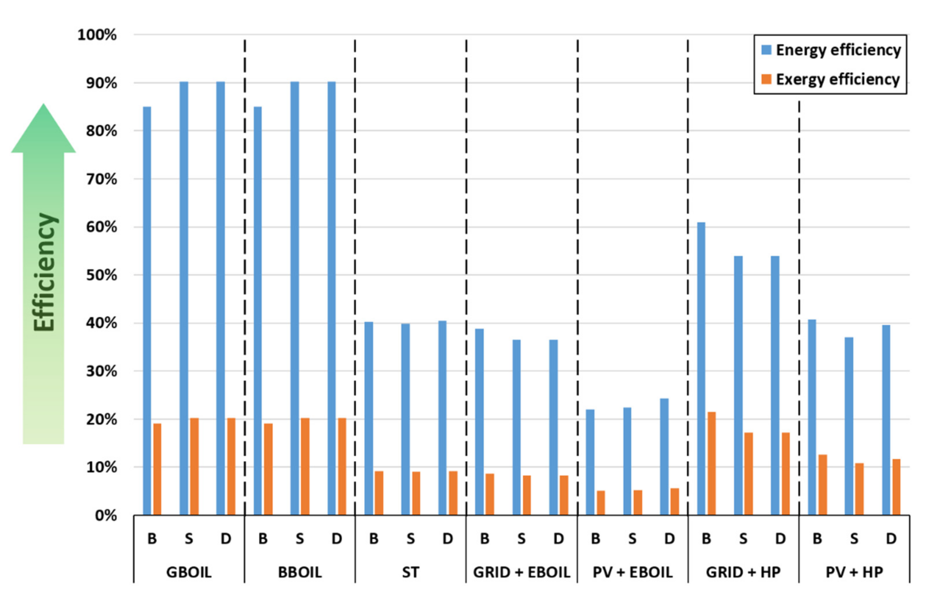
• From the viewpoint of energy efficiency, upscaling has mixed effects. On the one hand, specific efficiency increases for certain units, such as boilers or solar panels. On the other hand, large-scale implementation requires a district network that introduces additional losses, and in the case of heat pumps, a drop in performance due to higher temperature lifts. In solar-driven systems, upscaling enables demand pooling, with beneficial effects on overall performance. This pooling effect compensates for the drawbacks of upscaling at least partially and may even outweigh them in some instances. The pooling effect seems to be stronger between sectors than between buildings, due to the complementarity of residential and office demand profiles. In this specific study, upscaling led to relative increases of up to +11% in overall efficiency for some systems, but relative decreases of up to −11% for other systems, especially those involving a heat pump. The most efficient solutions were the biomass- and gas-fired boilers at large scales, with overall efficiencies of 90% (85% at building scale).
• From the viewpoint of exergy efficiency, the most efficient solution overall does not involve upscaling (grid-powered heat pumps at building scale, for 21.5% exergy efficiency). Biomass and gas boilers are the second-best solutions after upscaling (20.3%). The effects of upscaling on exergy efficiency are less promising than on energy efficiency: up to a +10% relative increase for certain systems, but up to a -20% relative decrease for other systems, especially those involving a heat pump. Nevertheless, maximizing the pooling effect can compensate for these drawbacks.
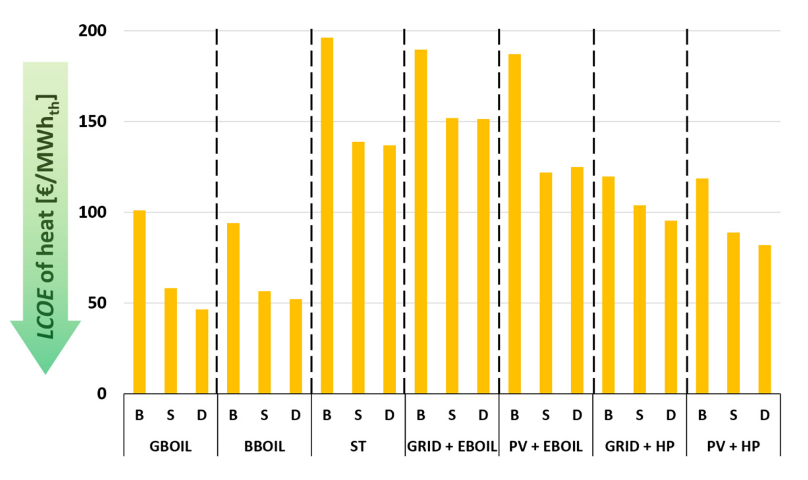
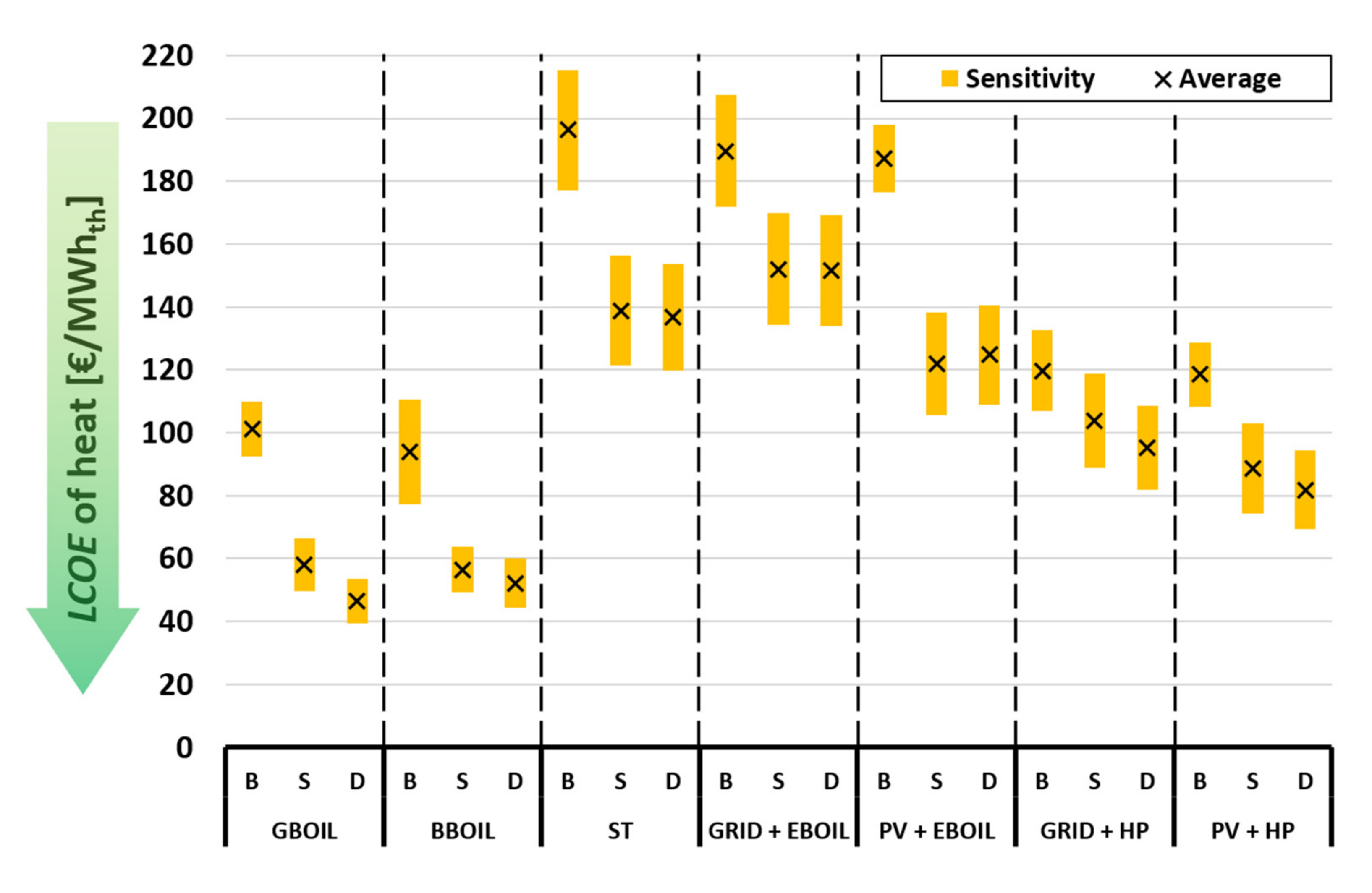
• From an economics viewpoint, upscaling and demand pooling lead to lower specific investment costs and fuel costs, reducing the LCOE of heat. In this study, the reduction was up to –54% with gas-fired boilers, −45% with biomass boilers, −35% with PV-powered electric boilers, −31% with PV-powered heat pumps, −30% with solar thermal collectors, −21% with grid-driven heat pumps, and −20% with grid-powered boilers. Upscaling yields more cost-efficient systems, even when accounting for some uncertainty in investment and fuel costs. Furthermore, upscaling hardly increases the sensitivity of the LCOE, and in some cases it even reduces it. Out of 21 systems evaluated in this study, the six most cost-efficient ones involved upscaling. The most promising system was a gas boiler plant at district scale.
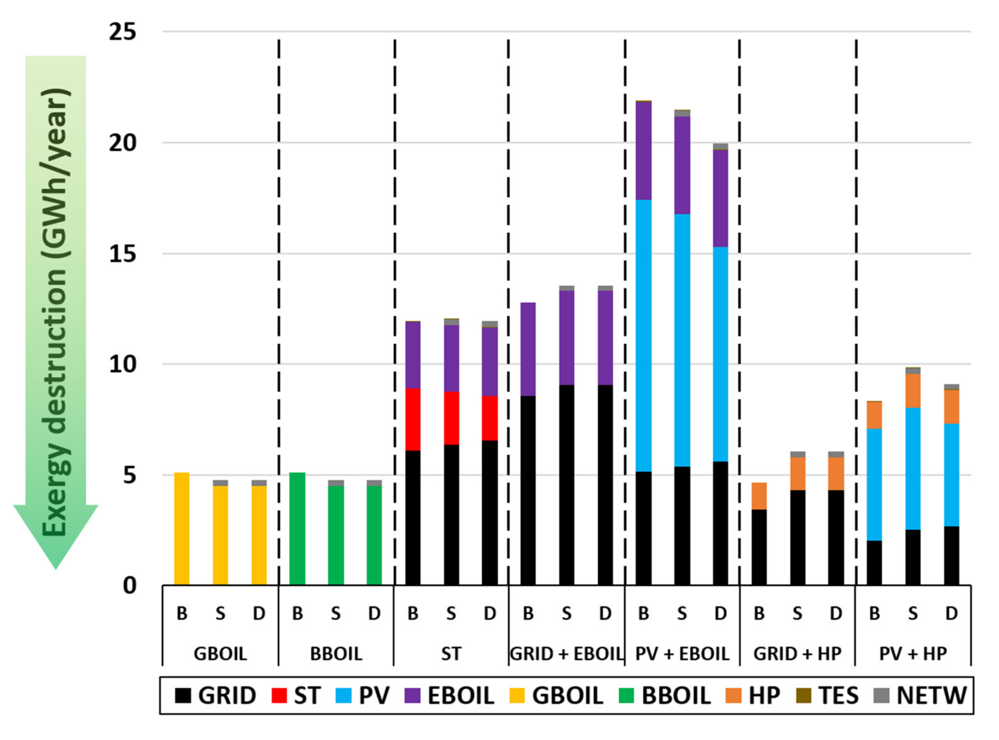
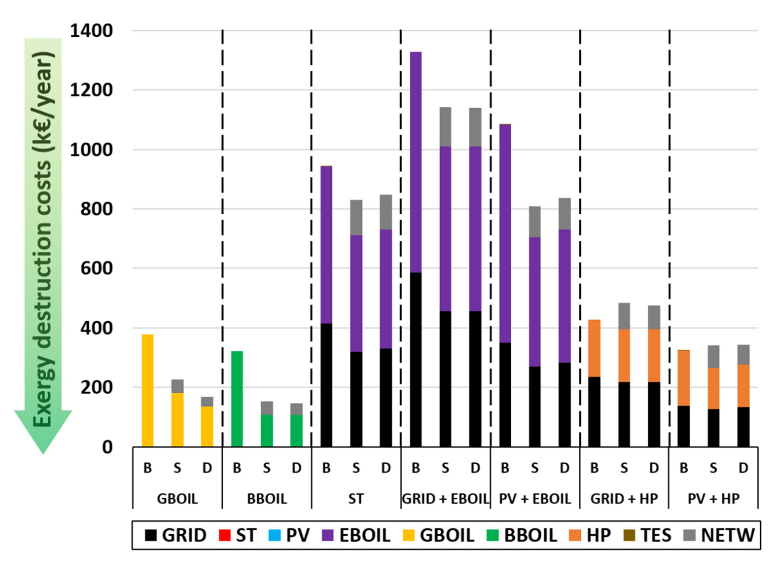
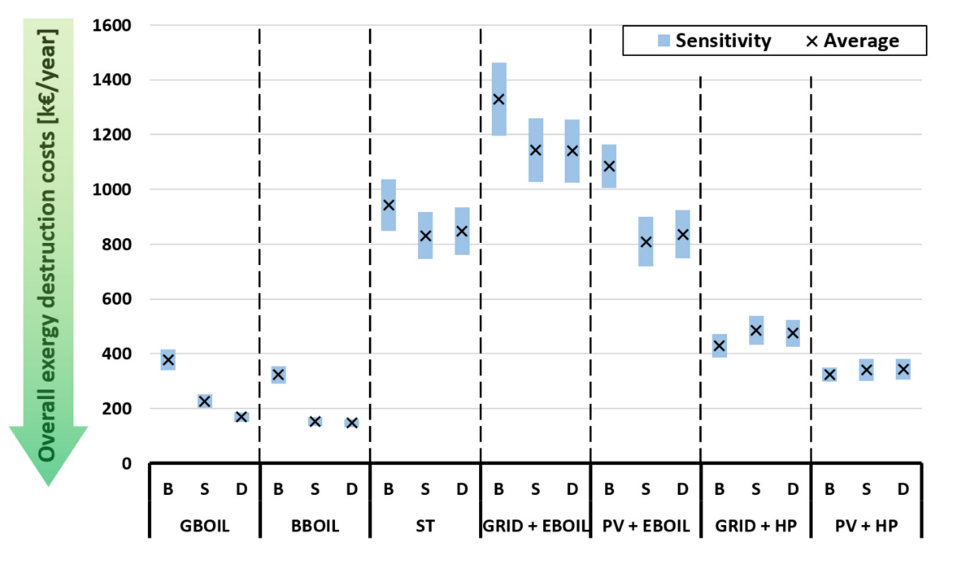
• From an exergoeconomic viewpoint, upscaling reduced exergy destruction costs for most of the systems, except those involving a heat pump. The reduction was up to −55% for biomass and gas boilers, −23% for PV-powered boilers, −14% for grid-powered boilers, and −10% for solar thermal collectors. On the other hand, exergy destruction costs increased by up to +13% and +6% for the grid-powered and PV-powered heat pumps, respectively. Out of 21 solutions, the best four involved upscaling. The most promising approach was a biomass-fueled boiler at district scale. Upscaling did not increase the sensitivity of exergy destruction costs, and in some instances, it even reduced it.
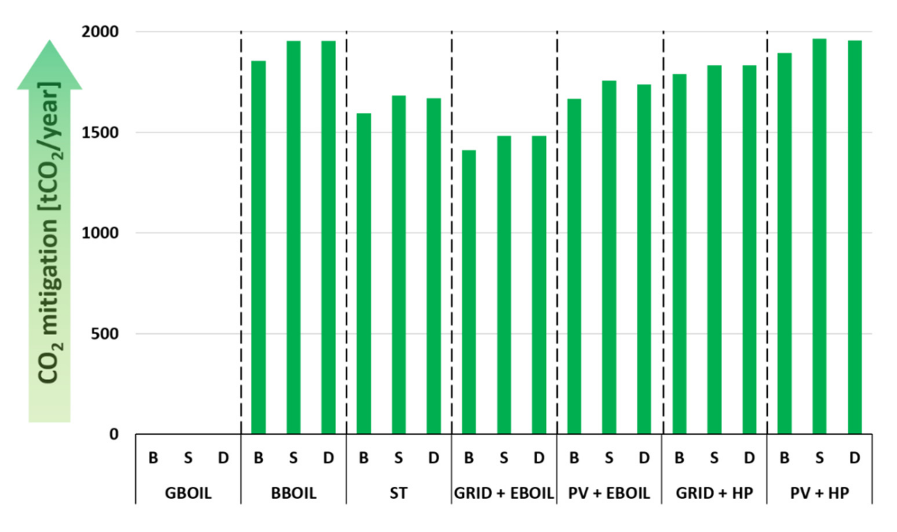
• From an environmental viewpoint, upscaling improved CO₂ mitigation by up to 5% in the current study. The improvement could be more substantial if embodied energy was taken into account. In this study, the systems with fewer emissions were biomass boilers and PV-powered heat pumps, and they were almost equivalent. The most promising approach consisted of PV-powered heat pumps at sector scale. The best four out of 21 solutions involved upscaling.

When comparing the technologies analyzed here, it appears that centralized biomass boilers and centralized PV-powered heat pumps represent the best compromise for efficient, environmental, and affordable heat production, depending on the context.

The authors’ main perspective is to analyze the effects of upscaling in different types of districts and within neighborhoods with different types of users. However, the results presented in this article are representative for an office district. It would be interesting to investigate its effects in an entirely residential district and in an evenly mixed district. In addition, it may be interesting to assess the performance of mixed solutions, combining several production units, as a function of the district composition. Transferring these results to other economic and electricity production scenarios in the grid context could entail revising our conclusions. However, the French energy market, which is highly reliant on nuclear power, may be representative of OECD countries in future conditions with high shares of non-carbon electricity. The effects of the sizing rules for production units and thermal storages could also be further investigated.

Another perspective would be to refine the working hypotheses for more applicable results, especially concerning the biomass boiler, temperature levels, and instantaneous performance of the units at each time step. For now, the study uses economic data by scale sizes, but profiles within the same scale have different peak powers. A more accurate approach would be to apply economic data by power tranches. However, such an approach can be time-consuming, as economic data by power tranches are scattered and need very refined modeling. Moreover, they may be unavailable depending on the building typology.

References

1. US EPA (United States Environmental Protection Agency). Global Greenhouse Gas Emissions Data. 2020. Available online: https://www.epa.gov/ghgemissions/global-greenhouse-gas-emissions-data (accessed on 1 March 2021).
2. European Commission. Climate Strategies & Targets, Climate Action—European Commission. 2016. Available online: https://ec.europa.eu/clima/policies/strategies_en (accessed on 1 March 2021).
3. The Government of Western Australia. Western Australian Climate Policy: A Plan to Position Western Australia for a Prosperous and Resilient Low-Carbon Future. 2020. Available online: https://www.wa.gov.au/sites/default/files/2020-12/Western_Australian_Climate_Policy.pdf (accessed on 1 March 2020).
4. National Conference of State Legislatures. Greenhouse Gas Emissions Reduction Targets and Market-Based Policies. 2019. Available online: https://www.ncsl.org/research/energy/greenhouse-gas-emissions-reduction-targets-and-market-based-policies.aspx#Introduction (accessed on 1 March 2020).
5. Zappa, W.; Junginger, M.; van den Broek, M. Is a 100% renewable European power system feasible by 2050? Appl. Energy 2019, 233–234, 1027–1050. [Google Scholar] [CrossRef]
6. ADEME. France Energy Efficiency & Trends Policies, Odyssee-Mure Project, a Part of EnR (European Energy Network), Co-Funded by H2020 Programme of the European Commission, Agence de l’Environnement et de la Maîtrise de l’Énergie (ADEME, French Agency for e. Available online: https://www.odyssee-mure.eu/publications/efficiency-trends-policies-profiles/france.html (accessed on 16 December 2021).
7. Harvey, L.D.D. A Handbook on Low-Energy Buildings and District-Energy Systems: Fundamentals, Techniques and Examples; Routledge: London, UK, 2012. [Google Scholar]
8. Ghafghazi, S.; Sowlati, T.; Sokhansanj, S.; Melin, S. A multicriteria approach to evaluate district heating system options. Appl. Energy 2010, 87, 1134–1140. [Google Scholar] [CrossRef]
9. Wang, H.; Yin, W.; Abdollahi, E.; Lahdelma, R.; Jiao, W. Modelling and optimization of CHP based district heating system with renewable energy production and energy storage. Appl. Energy 2015, 159, 401–421. [Google Scholar] [CrossRef]
10. Rämä, M.; Mohammadi, S. Comparison of distributed and centralised integration of solar heat in a district heating system. Energy 2017, 137, 649–660. [Google Scholar] [CrossRef]
11. Renaldi, R.; Friedrich, D. Techno-economic analysis of a solar district heating system with seasonal thermal storage in the UK. Appl. Energy 2019, 236, 388–400. [Google Scholar] [CrossRef] [Green Version]
12. Alsagri, A.S.; Arabkoohsar, A.; Khosravi, M.; Alrobaian, A.A. Efficient and cost-effective district heating system with decentralized heat storage units, and triple-pipes. Energy 2019, 188, 116035. [Google Scholar] [CrossRef]
13. Balić, D.; Maljković, D.; Lončar, D. Multi-criteria analysis of district heating system operation strategy. Energy Convers. Manag. 2017, 144, 414–428. [Google Scholar] [CrossRef]
14. Jonynas, R.; Puida, E.; Poškas, R.; Paukštaitis, L.; Jouhara, H.; Gudzinskas, J.; Miliauskas, G.; Lukoševičius, V. Renewables for district heating: The case of Lithuania. Energy 2020, 211, 119064. [Google Scholar] [CrossRef]
15. Fito, J.; Hodencq, S.; Ramousse, J.; Wurtz, F.; Stutz, B.; Debray, F.; Vincent, B. Energy- and exergy-based optimal designs of a low-temperature industrial waste heat recovery system in district heating. Energy Convers. Manag. 2020, 211, 112753. [Google Scholar] [CrossRef]
16. Fitó, J.; Russe, J.; Hodencq, S.; Wurtz, F. Energy, exergy, economic and exergoeconomic (4E) multicriteria analysis of an industrial waste heat valorization system through district heating. Sustain. Energy Technol. Assess. 2020, 42, 100894. [Google Scholar] [CrossRef]
17. Fitó, J.; Dimri, N.; Ramousse, J. Competitiveness of renewable energies for heat production in individual housing: A multicriteria assessment in a low-carbon energy market. Energy Build. 2021, 242, 110971. [Google Scholar] [CrossRef]
18. Fitó, J.; Dimri, N.; Ramousse, J. Effects of the sizing scale on the thermoeconomic and environmental performances of heat production systems for a mixed district in France. In Proceedings of the ECOS 2021 Conference, Taormina, Italy, 27 June–2 July 2021. [Google Scholar]
19. S Grand Chambéry. District of the Cassine, Yesterday, Today and Tomorrow, Consultation File Made Available to the Public. 2016. Available online: https://www.grandchambery.fr/epublication/104/23-dossier-de-concertation-quartier-cassine.htm?TELECHARGER=1 (accessed on 16 December 2021).
20. DES. Enquête Performance de l’Habitat, Équipements, Besoins et Usages de l’énergie (Phébus). SDES. 2013. Available online: https://www.statistiques.developpement-durable.gouv.fr/enquete-performance-de-lhabitat-equipements-besoins-et-usages-de-lenergie-phebus (accessed on 16 December 2021).
21. Profils Types de Demande de Chaleur et Monotone, Energie Plus Le Site. 2016. Available online: https://energieplus-lesite.be/donnees/cogeneration4/profils-types-de-demande-de-chaleur-et-monotone/ (accessed on 18 February 2021).
22. CEREN. Données Énergie 1990–2016 du Secteur Tertiaire; CEREN (The French Center for Economic Studies and Research on Energy): Paris, France, 2018. [Google Scholar]
23. CEREN. Précisions sur les Données du Tertiaire; CEREN (The French Center for Economic Studies and Research on Energy): Paris, France, 2018. [Google Scholar]
24. BEbio Construction, Détermination du Bbiomax et Cepmax—RT2012—Neuf. Available online: https://www.bebioconstruction.fr/wp-content/uploads/2015/09/Outil-de-calculs-du-Bbio-et-Cep.xls (accessed on 16 December 2021).
25. ADEME. Caractérisation des Consommations Energétiques des Bâtiments du Secteur Tertiaire Accueillant des Activités de Bureau et de Commerce. ADEME (The French Agency for Ecological Transition). 2008. Available online: https://librairie.ademe.fr/urbanisme-et-batiment/2036-caracterisation-des-consommations-energetiques-des-batiments-du-secteur-tertiaire-accueillant-des-activites-de-bureau-et-de-commerce.html (accessed on 16 December 2021).
26. ADEME; COSTIC. Les Besoins d’eau Chaude Sanitaire en Habitat Individuel et Collectif. ADEME (The French Agency for Ecological Transition). Available online: https://www.ademe.fr/sites/default/files/assets/documents/besoin-eau-chaude-sanitaire-habitat-individuel-et-collectif-8809.pdf (accessed on 16 December 2021).
27. INSEE. Taille des Ménages dans l’Union Européenne, Annual Data from 2004 to 2018. INSEE (The French National Institute of Statistics and Economic Studies). 2020. Available online: https://www.insee.fr/fr/statistiques/2381488 (accessed on 16 December 2021).
28. Energie Plus. Consommation d’eau Chaude Sanitaire. 2007. Available online: https://energieplus-lesite.be/donnees/consommations2/consommation-d-eau-chaude-sanitaire/ (accessed on 1 March 2021).
29. Centre Scientifique et Technique du Bâtiment (CSTB): ANNEXE—Méthode de calcul Th-BCE 2012 [Annex to the calculation method Th-BCE2012]. J. Off. 2011, 77, 1377. Available online: https://www.e-rt2012.fr/wp-content/uploads/fichiers/methode-calcul-thbce-rt-2012-cstb.pdf (accessed on 16 December 2021).
30. Lund, H.; Werner, S.; Wiltshire, R.; Svendsen, S.; Thorsen, J.E.; Hvelplund, F.; Mathiesen, B.V. 4th Generation District Heating (4GDH). Energy 2014, 68, 1–11. [Google Scholar] [CrossRef]
31. ADEME. Les Réseaux de Chaleur et de Froid—État des Lieux de la Filière. Technical Report, Agence de l’Environnement et de la Maîtrise de l’Énergie. ADEME (The French Agency for Ecological Transition). 2019. Available online: https://librairie.ademe.fr/energies-renouvelables-reseaux-et-stockage/818-reseaux-de-chaleur-et-de-froid-etat-des-lieux-de-la-filiere-marches-emplois-couts.html (accessed on 16 December 2021).
32. Hodencq, S.; Brugeron, M.; Fitó, J.; Morriet, L.; Delinchant, B.; Wurtz, F. OMEGAlpes, an open-source optimisation model generation tool to support energy stakeholders at district scale. Energies 2021, 14, 5928. [Google Scholar] [CrossRef]
33. Pajot, C.; Morriet, L.; Hodencq, S.; Delinchant, B.; Maréchal, Y.; Wurtz, F.; Reinbold, V. OMEGAlpes: An optimization modeler as an efficient tool for design and operation for city energy stakeholders and decision makers. Build. Simul. Conf. Proc. 2019, 4, 2683–2690. [Google Scholar] [CrossRef]
34. Delinchant, B.; Hodencq, S.; Marechal, Y.; Morriet, L.; Pajot, C.; Wurtz, F. OMEGAlpes Documentation. Available online: https://omegalpes.readthedocs.io/en/latest/ (accessed on 16 December 2021).
35. Rajoria, C.S.; Agrawal, S.; Tiwari, G.N. Exergetic and enviroeconomic analysis of novel hybrid PVT array. Sol. Energy 2013, 88, 110–119. [Google Scholar] [CrossRef]
36. UK Parliament. Carbon Footprint of Heat Generation. 2016. Available online: https://post.parliament.uk/research-briefings/post-pn-0523/ (accessed on 23 July 2020).
37. Huld, T.; Müller, R.; Gambardella, A. A new solar radiation database for estimating PV performance in Europe and Africa. Sol. Energy 2012, 86, 1803–1815. [Google Scholar] [CrossRef]
38. Guillerminet, M.-L.; Marchal, D.; Gerson, R.; Berrou, Y. Coûts des Energies Renouvelables en France. ADEME (The French Agency for Ecology Transition). 2016. Available online: https://www.ademe.fr/sites/default/files/assets/documents/couts_energies_renouvelables_en_france_edition2016v1.pdf (accessed on 16 December 2021).
39. ADEME. Rénovation: Se Chauffer Mieux et Moins cher. ADEME (The French Agency for Ecology Transition). 2019. Available online: https://librairie.ademe.fr/urbanisme-et-batiment/2215-se-chauffer-mieux-et-moins-cher-9791029707582.html (accessed on 16 December 2021).
40. ADEME. Modes de Chauffage dans l’habitat Individuel. ADEME (The French Agency for Ecology Transition). 2014. Available online: https://librairie.ademe.fr/urbanisme-et-batiment/2973-modes-de-chauffage-dans-l-habitat-individuel.html (accessed on 16 December 2021).
41. Kalogirou, S.A. Solar Thermal Collectors and Applications. Prog. Energy Combust. Sci. 2004, 30, 231–295. [Google Scholar] [CrossRef]
42. Bayrak, F.; Abu-Hamdeh, N.; Alnefaie, K.A.; Öztop, H.F. A review on exergy analysis of solar electricity production. Renew. Sustain. Energy Rev. 2017, 74, 755–770. [Google Scholar] [CrossRef]
43. Fleiter, T.; Jan, S.; Mario, R.; Andreas, M. Mapping and Analyses of the Current and Future (2020–2030) Heating/Cooling Fuel Deployment (Fossil/Renewables), Work Package 2: Assessment of the Technologies for the Year 2012; European Commission: Brussels, Belgium, 2016. [Google Scholar] [CrossRef]
44. Gudmundsson, O.; Thorsen, J.E.; Zhang, L. Cost analysis of district heating compared to its competing technologies. WIT Trans. Ecol. Environ. 2013, 176, 107–118. [Google Scholar] [CrossRef] [Green Version]
45. Dimri, N.; Ramousse, J. Thermoeconomic optimization and performance analysis of solar combined heating and power systems: A comparative study. Energy Convers. Manag. 2021, 244, 114478. [Google Scholar] [CrossRef]
Figure 1. Boundary mapping (© OpenStreetMap contributors - licensed under the Open Data Commons Open Database License–OdbL-by the OpenStreetMap Foundation-OSMF)and distribution of annual space heating and DHW demands of the Cassine district located in Chambéry, France.
Energies 14 08546 g001
Figure 2. Schematic representation of the three approaches considered for sizing the heat production units.
Energies 14 08546 g002
Figure 3. Overall energy and exergy efficiencies for each solution, at each scale size. D = District-scale sizing; S = Sector-scale sizing; B = Building-scale sizing.
Energies 14 08546 g003
Figure 4. Overall LCOE of heat for every solution at every scale. D = district-scale sizing; S = sector-scale sizing; B = building-scale sizing.
Energies 14 08546 g004
Figure 5. Overall CO2 mitigation for every solution at every scale.
Energies 14 08546 g005
Figure 6. Exergy destruction, overall and unit-by-unit, for every solution at every scale.
Energies 14 08546 g006
Figure 7. Exergy destruction costs, overall and unit by unit, for each solution at each scale.
Energies 14 08546 g007
Figure 8. Sensitivity of LCOE to variations in investment and fuel costs.
Energies 14 08546 g008
Figure 9. Sensitivity of exergy destruction costs to variations in investment and fuel costs.
Energies 14 08546 g009