Article

Experimental and Numerical Study of Multiple Jets Impinging a Step Surface

by
Flavia V. Barbosa
1,*,
Senhorinha F. C. F. Teixeira
2 and
José C. F. Teixeira
1
1
MEtRICs I&D Centre, School of Engineering, University of Minho, 4800-058 Guimarães, Portugal
2
ALGORITMI I&D Centre, School of Engineering, University of Minho, 4800-058 Guimarães, Portugal
*
Author to whom correspondence should be addressed.
Energies 2021, 14(20), 6659; https://doi.org/10.3390/en14206659
Submission received: 18 September 2021 / Revised: 7 October 2021 / Accepted: 12 October 2021 / Published: 14 October 2021

Abstract

:
Multiple jet impingement is a widely implemented convective process for enhancing heat transfer over target surfaces. Depending on the engineering application, the impinging plate can have different configurations. However, the increased complexity of the surface induces complicated thermal behaviors that must be analyzed. In that sense, this study consisted of the experimental and numerical analysis of multiple jets impinging on a step surface. A particle image velocimetry technique was applied to measure velocity fields, while a heat flux sensor was mounted on the surface to determine the heat transfer. Numerical simulations, for both flat and non-flat plates, were conducted in ANSYS FLUENT applying the SST k-ω model, and experimental results were used to validate the model. Three surface configurations were analyzed, flat, 1 D, and 2 D steps, and the results show an increase in the average Nusselt number compared with the flat plate, 9% and 20%, respectively. This increase was mainly due to the intensification of the flow turbulence induced by the step. Numerical results were in good agreement with the experiments, but the heat transfer was slightly underpredicted for the 2 D step case due to the difficulty of predicting with accuracy the velocity field near the step.

Graphical Abstract

1. Introduction

The consumption growth of electronic products has increased the demand for printed circuit boards (PCBs) [1]. In addition, the expansion of the electronic products market has led to an increase in the complexity of PCBs, which causes a more complex thermal response when a PCB passes through a reflow oven [2]. Inside this equipment occurs a process known as reflow soldering, which is achieved by forced convection using multiple air jet impingement technologies [3]. This process is currently the primary manufacturing technology used for the attachment of electronic components to the PCB by melting the solder paste, allowing the connection between the board and the components. However, it is observed that inhomogeneous thermal distribution emerges during the reflow soldering around and within the components, essentially due to the variability of their dimensions and the high thermal capacity, leading to soldering failures [4]. In practice, defective products require repairs and reworking that can cause a loss of productivity and an increase in the total manufacturing costs of 30% to 50% [5]. In that sense, it is evident that target plate geometry plays an important role in the heat transfer efficiency of the reflow soldering process. To enhance the convective heat transfer and minimize the defects, studies have been conducted to understand the effect of complex surfaces on multiple jet impingement flow dynamics and heat transfer.
Caliskan and Baskaya [6] investigated heat transfer in an inline jet array (2000 < Re < 10,000) on smooth and rib-roughened surfaces according to two configurations: V-shaped ribs (V-SR) and convergent-divergent shaped ribs (CD-SR). Through their analysis, they concluded that both configurations increase the heat transfer coefficient over the surface from 4% to 26.6% when compared with a flat plate. Their results show that a V-SR configuration presented a higher average heat transfer than CD-SR since this structure generated vortices that increased the flow mixing, enhancing the heat transfer. V-SR disturbs the boundary layer induced by the jet impingement inside the rib cavity, which creates higher turbulence, especially for a nozzle-to-plate distance of 2 (H/D = 2). Chauhan and Thakur [7] studied the heat transfer and friction factor correlations for impinging jets (3800 < Re < 16,000) and observed that the streamwise and spanwise jet-to-jet spacing that enhanced the heat transfer rates and friction factors were Sx/D = 1.74 and Sy/D = 0.87. These results highlight the effect of this variable on the formation of the impingement boundary layer generated in the vicinity of the target surface. Nayak and Singh [8] analyzed the effect of geometrical aspects on the performance of impinging jets (2700 < Re < 6900) for different crossflow configurations, jet-to-plate spacing, and mass flow rate, and they found that the heat transfer increased for large H and high mass flow rates. Buzzard et al. [9] evaluated the combination of small rectangular shape roughness with a larger rectangular pin (900 < Re < 11,000) and concluded that the heat transfer was enhanced by small rectangle roughness since the local vorticity and the mixing between ambient air and the jet flow was increased by these structures. Alenezi et al. [10] and Tepe et al. [11] highlighted the importance of rib height since ribs that were too high could induce a lower heat transfer rate when compared with flat plates. In this case, the flow must travel a longer distance between the wall and the upper edge of the rib before re-attachment. In that sense, it seems that a rib height that matches with the boundary layer thickness and is located between the stagnation region and the wall jet region enhances the local heat transfer mainly due to the increased turbulence due to the flow recirculation before and after the rib [10]. Yuan-Hsiang and Yao-Hsien [12] experimentally investigated the heat transfer distribution from multiple jets impinging on target plates with different roughness, for 2500 < Re < 7700. The authors found that the change in surface geometry broke the flow development and enhanced the flow mixing. Their study showed that surfaces with partial roughness increased the heat transfer by 50% for the case of longitudinal grooves. Nadda et al. [13] compared different surface geometries and verified that multiple arc protrusion rib geometry generated the best heat transfer performance in impingement jets. A recent research study conducted by Ren et al. [14] (1000 < Re < 15,000) mentioned that a surface with square pin fins could increase the heat transfer by 20% to 300% compared with a flat plate, mainly due to the thermal transport and near-wall mixing. The increased wetted area and the increased turbulence intensity caused by the breaking of the viscous sublayer were additional factors that enhance the heat transfer. Nagesha et al. [15], for 10,000 < Re < 27,500, demonstrated that the heat transfer enhancement in rough target surfaces was due to the area increase and to turbulence enhancement. However, this enhancement depended on the target shape. For example, while multi-protrusions increased the turbulence generation, this increase was not observed in V-grooves due essentially to the air trapped inside the cavities. These studies allow the conclusion that non-flat plates increase the complexity of the flow field and that in some cases the heat transfer is enhanced, while in others both heat transfer and surface coverage can be reduced.
Considering the complexity of the multiple jets impinging on non-flat plates, numerical models have been developed in order to predict the physical phenomena, reducing the number of experiments. Modelling turbulent flows is very challenging and most of the numerical codes are Eulerian based. However, there have been interesting developments on Lagrangian methods [16,17]. According to [17], this method presents advantages in terms of being much less dissipative than Eulerian counterparts on the advection term of the Navier–Stokes equations. Even though the Lagrangian method presents promising results for the modeling of turbulent flows and heat transfer, Eulerian methods have been extensively applied over recent years, and several models have been implemented on the jet impingement field [10,18,19,20,21,22,23,24]. From the different numerical methods—direct numerical simulation (DNS), large eddy simulation (LES), and Reynolds-averaged Navier–Stokes (RANS)—RANS is the most used method since it provides fairly accurate results at low computational costs. From the different turbulence models presented in the literature, the SST k-ω model, developed by Menter [25], was revealed to be both accurate and computing time-saving in engineering applications; therefore, it was implemented in this work.
Even if different plate geometries have been analyzed both experimentally and numerically, no work has focused on step surfaces. To complement the research on multiple air jets impinging on complex target surfaces, this work focused on the characterization of the jets’ flow dynamics and heat transfer over surfaces with a step and compared the results obtained with a flat plate. To perform the study, experiments using a particle image velocimetry (PIV) technique were conducted for a Reynolds number of 5000, a nozzle-to-plate distance (H/D) equal to 2, and a jet-to-jet spacing (S/D) equal to 3. From the experiments, the flow was characterized and the influence of the step configuration on heat transfer performance and surface coverage was determined. Experiments were used to validate the model that was developed, with analysis using ANSYS FLUENT software.

2. Experimental Method

This section describes the experimental setup used to conduct the experiments as well as the methodologies implemented to characterize the flow field and heat transfer of multiple air jets impinging on different target surface configurations.

2.1. Experimental Apparatus

The experimental apparatus was specially designed and constructed to perform a detailed study of multiple air jets impinging on flat and non-flat target surfaces. Two methodologies were applied in this study: the measurement of velocity fields using the PIV technique to determine the jets’ flow dynamics, providing detailed information on the overall flow, and the measurement of the average heat transfer using a heat flux sensor. Both measurement techniques are detailed in the following sections.
As depicted in Figure 1a,b, the experimental apparatus consisted of a centrifugal fan that blew the ambient air into the test rig. An acrylic settling chamber was linked to the fan to reduce the turbulence of the flow and a honeycomb structure was implemented to direct the flow towards the measurement chamber. A long, square section, acrylic tube allowed the uniformization of the flow in order to ensure that the same flow rate fed the orifice nozzles. The configuration of the nozzle plate, which was located at the bottom of the tube, could be adapted in function of the jet-to-jet spacing in analysis. As the air flowed through the nozzles, turbulent jets were produced. The Reynolds number and the turbulence intensity measured at the nozzles exit were approximately equal to 5000 and 6%, respectively. As the jets approached the target plate and, after the impingement, the flow developed over the wall. Depending on the configuration of the impinging plate, the complexity of the flow increased. Two configurations were analyzed in this work: flat and non-flat plates, as depicted in Figure 2. The last one consisted of a step surface with a height equal to 1 D and 2 D. The impingement section was open, meaning that free outflow of the air was allowed in all directions. A mica heater plate was used to heat the target plate, and its temperature control was ensured by a Selec TC544 temperature controller.

2.2. PIV Measurements

The measurement of the velocity field was conducted using a non-intrusive method—the PIV technique—schematically presented in Figure 3. Seeding particles of olive oil with a diameter varying between 1 and 3 μm were mixed with the air in order to provide accurate flow tracking and a good light scattering from a two-dimensional laser sheet induced by a Nd:YAG laser. The tracking particles diameter was optimized in order to ensure an accurate flow tracking as well as an optimum light scattering, minimizing the influence of the olive oil on the air, following the recommendation presented by [26]. The seeding was generated by an Aerotech Smoke Generator that delivered particles to the system at a mass flow rate of approximately 5 g/h. A CCD camera captured the motion of the particles by the acquisition of two consecutive images recorded at a short time between pulses [27]. The images were divided into interrogation areas and mathematical correlations were applied on the cluster of the tracking particles within each area between the two frames, yielding a signal peak that represented the particle displacement [28]. The velocity vectors were generated using the adaptative correlation method. This method iteratively adjusted the size and shape of the interrogation area (IA), applying refinement steps, and used the information of the intermediary results between a larger and a smaller IA until the final size was obtained [29]. In this study, the interrogation area size was varied from 128 × 128 pixels to 32 × 32 pixels, with 3 refinement steps and an overlap of 50% in both horizontal and vertical directions. According to Cao et al. [30], these values lay between the typical range implemented for indoor airflow PIV applications.

2.3. Heat Transfer Measurements

The heat flux was measured using an OMEGA® HFS-4 thin film heat flux sensor, which was mounted at the center of the target plate (Figure 4). The heat flux sensor was based on a thermopile formed around an electrically insulating layer. A large number of thermocouple pairs were connected in series measuring the temperature difference across the thermal barrier which was proportional to the heat flow through the sensor [31]. This sensor followed Fourier’s law of thermal conduction to determine the heat flux, as expressed in Equation (1). The average heat flux, q ¯ , was determined across a known thickness, Δx, of material whose thermal conductivity, k, was provided by the manufacturer [32].
q ¯ = k d T d x k d T d x
where ΔT is the temperature difference measured by the thermocouples across a known thickness of Kapton® material, Δx = 0.18 mm, whose thermal conductivity was considered equal to k = 0.045 W/m·K, according to the manufacturer information. Moreover, the information provided indicated that the heat flux sensor output for a temperature close to 120 °C, which represents the operating temperature achieved by the target plate, was equal to 1.8 µV/W/m2. The heat flux and temperature measurements were recorded by a NI 9213 data acquisition system. An algorithm was written using the LabVIEW-based software to process the data and values of temperature and heat flux in function on time were obtained and analyzed.
The scheme presented in Figure 5 shows the position of the heat flux sensor in relation to the nozzles. As can be observed, only a portion of the total jets impinged the sensor. The average heat transfer was obtained by averaging the contribution of seven nozzles within its footprint which was representative of the whole target plate. Therefore, the heat flux measured was a representative value of the mean over the target plate. Furthermore, as depicted in Figure 5a, the sensor was placed in the vicinity of the step to ensure that the influence of the step on the heat transfer was captured.

2.4. Experimental Method

The experiments were carried out at an ambient temperature, 25 °C, and a relative humidity varying between 40% and 60%. The Reynolds number, calculated at the nozzle, was equal to 5000, a fully turbulent regime. The heater worked on an on–off basis, being operated by a Selec TC544 temperature controller with an accuracy of 0.25% of full-scale. The input temperature was provided by a thermocouple attached to the plate which was mounted at a specific distance from the impinging region to avoid interference from that the jets’ flow, ensuring an operating temperature of 120 °C. The measured variables, the heat flux, air jets, and plate temperatures, were recorded over a time span of 30 min. It was observed that the plate temperature stabilized at 120 °C after 10 min of experiment. Therefore, the stabilization period started from this moment until the end of the test. The temperature difference used to determine the heat transfer over the target plate was provided by the plate temperature and the temperature of the jets, which was measured at the stabilization chamber to ensure that the temperature of the plate did not interfere with the air jets’ temperature.
To conduct the PIV measurements, the central row of the nozzle plate was analyzed. In order to ensure accurate flow field measurements, the CCD camera was focused on the central jet and two adjacent jets. Since the jets’ pattern was staggered, the interactions between the flow of the jets located on the back and front rows and the central jets were also captured. The target plate was cleaned between each experiment to ensure that no seeding particles interfered with the heat transfer measurements.

2.5. Data Reduction and Uncertainty Estimation

The average Nusselt number was determined as a function of the average convective heat transfer coefficient, h ¯ , the nozzle diameter, D, and thermal conductivity of the air, k, according to Equation (2). While the nozzle’s diameter was a constant geometrical parameter and k was temperature-dependent and obtained directly from the literature [33], h ¯ had to be calculated by applying Equation (3).
Nu ¯ = h ¯ · D k
h ¯ = q ¯ T w ¯ T j ¯
where q ¯ is the average heat flux measured by the heat flux sensor, T w ¯ represents the average plate temperature, and T ¯ j is the average jet’s temperature.

2.5.1. PIV Measurements

The velocity, U , measured by the PIV system was composed of two components, in x and y directions, being the uncertainty related to both components expressed by u Ux and u Vy , respectively. Since the uncertainty quantification method was the same for both velocity components, u Ux = u Vy = u U was considered. According to [34], the velocity uncertainty depends on the time between pulses, Δt, the magnification factor, ΔS, and the particles displacement, Δxp. Therefore, the PIV uncertainty can be quantified as Equation (4):
u U = U Δ S u Δ S 2 + U Δ x p u Δ x p 2 + U Δ t u Δ t 2
Since the time between pulses Δt, can be considered infinitely small, for a certain range of flow turbulence, its contribution to the velocity uncertainty can be neglected. Moreover, [35] referred that, if the calibration is conducted properly, the magnification and calibration uncertainties are considered negligible when compared with the total uncertainty. Therefore, the total uncertainty is dominated by the displacement term and Equation (4) can be simplified, becoming Equation (5):
u U = U Δ x p u Δ x p 2
Systematic errors in PIV are difficult to determine since they can be caused by several sources, such as out-of-plane motion, scattering of tracer particles, and background, among others [36]. In contrast, random errors can be estimated by repeating an experiment a number of times and then evaluating how the result fluctuates. As mentioned by [37], PIV has matured enough to be considered bias-free if used properly. Therefore, only the random errors are considered for uncertainty quantification. The random errors in PIV measurements are due to horizontal and vertical displacement, u Ux , and   u Vy , respectively. These errors are assumed to be independent and normally distributed with zero mean and standard deviation σ. The resultant random error, u U , follows a Rayleigh distribution and is given by the square root of the squared random errors, u Ux and   u Vy , as expressed in Equation (6) [37]. For this analysis, u U was determined considering a level of confidence of 95%. A total sample number, N, equal to 300 was considered, being the 95% confidence achieved with an expansion factor equal to kp = 1.96 [38], according to Equation (7). This equation was used for u Ux and   u Uy considering a standard deviation σ Ux and σ Vy , respectively.
u U   = u Ux 2 + u Vy 2 .
u Ux , Vy   = k p · σ Ux , Vy N
The maximum uncertainty was obtained where maximum velocities were recorded as being close to 10%. The uncertainty of the measurement was expected to decrease with an increase in the sample size. According to [39], 2000 samples were a good size for reducing the uncertainty of the time-averaged velocities, u and v.

2.5.2. Heat Transfer Measurements

The uncertainty associated with the heat transfer measurements, and estimated for 95% of confidence level, was obtained using the ASME 98 methodology [38], also applied by [36].
Considering that the Nusselt number is a dependent variable obtained by h ¯ , D, and k , its uncertainty was determined by Equation (8). In turn, h ¯ depends on q ¯ , T w ¯ and T j ¯ , and so it was estimated by Equation (9).
u N u = N u h ¯ · u h 2 + N u D · u D 2 + N u k · u k 2
u h = h   q ¯ · u q ¯ 2 + h Δ T · u Δ T 2
while q ¯ , T w ¯ , and T j ¯ were measured directly by the heat flux sensor and thermocouples, D resulted from the diameter measurement of 10 circular nozzles, while k was directly obtained from the literature [33]. This parameter varies linearly with temperature (20 °C < Tj < 35 °C); therefore, it could be calculated for each air jet’s temperatures through Equation (10). This equation was obtained from a linear regression of the tabled thermal conductivity values data in function of air temperature (Tj).
k = 7.00 × 10 5 · T j + 2.37 × 10 2
u   q ¯ ,   u Δ T ,   u h ,   u D ,   u k   (Equations (8) and (9)) represent the uncertainty of the heat flux, temperature, heat transfer coefficient, nozzle diameter, and thermal conductivity, respectively. Since the total uncertainty was obtained by random and systematic errors, the random component of the uncertainty, ε , associated with u   q ¯ ,   u Δ T ,   u D , was calculated using Equation (11) [40], while the systematic part assumed the values presented in Table 1. These values were obtained by a rectangular distribution of the specifications provided by the manufacturers, according to [40].
ε = k p · σ N
where σ is the standard deviation of the measured data, and kp is the expansion factor obtained by means of a t-Student distribution for 95% and using the degrees of freedom (DOF) (i.e., DOF = N − 1), in which N represents the samples number.

3. Numerical Method

The numerical simulations were conducted using the commercial software, ANSYS FLUENT [41]. This section describes the governing equations, physical domain, and boundary conditions implemented in the numerical model as well as the numerical techniques applied.

3.1. Governing Equations

The Reynolds-averaged Navier–Stokes (RANS) equations were solved using ANSYS FLUENT 2020 R1 software. Since the flow was incompressible (a Mach number below 0.3 was ensured in all simulations), the equations of continuity (12), momentum (13), and energy (14) can be written using vectors notation as follows:
· u = 0
u t + u · u = 1 ρ p + μ 2 u
T t + u · T = κ 2 T
where u is the velocity vector, p is the fluid pressure field, and T the temperature. ρ, µ, and κ are constant physical properties of the fluid and represent the density, kinematic viscosity, and thermal diffusivity, respectively. These variables were defined for air at ambient temperature, 25 °C, according to [33].

3.2. Physical Domain and Boundary Conditions

As expressed in Figure 6a, the physical domain consisted of 17 confined air jets, H/D = 2, and S/D = 3, impinging on a flat and non-flat plate; more details regarding the non-flat surface are presented in Figure 6b. The air flowed through circular nozzles at a constant velocity (15 m/s) and temperature (25 °C), leading to a Reynolds number of approximately 5000, while the nozzle plate was defined by no-slip and adiabatic boundary conditions. The jets cooled the target plate, which was characterized by a constant temperature of 120 °C and a no-slip boundary condition. Since the jets array that was modelled corresponded to a portion of the experimental setup, as mentioned in Section 2.4, a symmetry condition was applied to the side walls of the domain, as shown in Figure 6.

3.3. Turbulence Modelling

Several authors agree that the RANS type SST k-ω model is both accurate and computing time-saving for the modeling of multiple jet impingement systems [42,43,44,45,46]. In that sense, this turbulence model was implemented in this work.
The SST k-ω model, developed by Menter [25], applied the k-ω model in the near-wall region and switched to the k-ε model in the far field, combining the advantages of both models. The combination between the SST and the k-ω models improved the near wall treatment since it gradually switched from a classical low-Reynolds formulation on fine meshes to a log-wall function formulation on coarser grids [47]. To describe the flow near a wall, the SST k-ω model used a low-Reynolds number approach allowing a detailed description of the viscous sublayer [18,47]. This low-Re approach is relevant for flows that lie in the transition regime or flows with low turbulence, such as the flow applied in this study. However, the SST k-ω model presents accurate results for highly turbulent flow (Re > 10,000), as presented by [11,44,46]. Equations (15) and (16) express the turbulence kinetic energy, k, and the specific dissipation rate, ω, respectively.
t ρ k + x i ρ k u i = x j Γ k k x j + G k Y k + S k
t ρ ω + x i ρ ω u i = x j Γ ω ω x j + G ω Y ω + S ω + D ω
where Γ represents the effective diffusivity, G is the generation, and Y is the dissipation of the corresponding variables; S is the user-defined source terms, while Dω is the cross-diffusion term [48].

3.4. Discretization

A second-order upwind scheme was used for the spatial discretization of all diffusion and convective terms. To compute the face values of pressure from the cell values, a second-order interpolation scheme was implemented using a central differencing scheme. The spatial discretization of the convection and diffusion terms was ensured by a least squares cell-based gradient evaluation. Pressure-velocity coupling was applied to derive an additional condition for pressure, and a procedure similar to that outlined by Rhie and Chow [49] was used to prevent checkerboarding [50]. The pressure-based solver applied the SIMPLE method to couple the pressure and velocity. The simulation was transient, so the governing equations were discretized in time through a first-order implicit integration. To perform the transient calculations, an adaptative time step was used. This method adjusted the time step size in function of the truncation error. If the truncation error was smaller than 0.01, the size of the time step was increased, while if the truncation error was greater, the time step size was decreased. The truncation error-based method was selected instead of the CFL method since it presented a suitable accuracy and lower computational time. Moreover, the constant truncation error value was defined based on preliminary studies, which compared different values and the simulation time, finding that an error equal to 0.01 presented good predictions at a lower simulation time.

3.5. Grid Independency

An analysis of the grid independence on the numerical calculations is analyzed in this section. The simulations were conducted on three consecutively refined grids, presented in Table 2. All grids consisted of square elements with refinement applied near the nozzle plate and the target surface to ensure that the shear layer generated at the exit of the jets and the development of the boundary layer over the surface were accurately predicted. Moreover, considering that the SST k-ω model was applied, the near-wall grid quality had to be ensured. Therefore, the value of the dimensionless distance between the first node and the wall, known as the y+ factor, had to be lower than 2 [48]. As can be observed in Table 2, only the medium and fine grids complied with this requirement.
The variable considered for the grid independence test was the average Nusselt number over the plate, and the results are presented in Figure 7. The heat transfer area considered for this analysis corresponded to half the surface impinged by the central jet, in which x/D = 0 represented the central jet axis. The results reveal a typical heat transfer behavior of a jet impingement in a highly confined space [51]. Furthermore, as the grid was refined, the variation of Nu ¯ became less pronounced. The higher deviation between the medium and the fine mesh was identified near the stagnation point (x/D = 0), with a maximum difference equal to 7%. Considering this slight difference between the predictions of the medium and fine mesh, and since the number of elements was about 30% higher in the fine mesh, the medium mesh was selected to conduct the numerical simulations. The complexity of the flow was expected to increase with the non-flat plate. However, since a near wall grid quality was ensured (y+ < 2)—and considering that the number of elements applied in previous studies, which modeled roughened surfaces with the SST k-ω [10,44,46], was close to the one applied in this study—the mesh used for the flat plate case was also implemented for the non-flat plate.

3.6. Numerical Algorithm

ANSYS Fluent® solved the Navier–Stokes and energy equations using the finite volume method and the discrete values of any variable were stored at the cell centers. Since the governing equations were non-linear and coupled to one another, the solution process involved iterations wherein the entire set of governing equations was solved repeatedly until the solution converged. To solve these equations, a pressure-based coupled algorithm was implemented. Since in coupled algorithm the momentum and continuity equations are solved in a closely coupled manner, the rate of solution convergence significantly improved compared with other algorithms, such as pressure-based segregated [41].

4. Results and Discussion

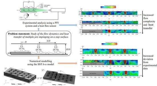
In this section, the jets’ flow dynamics and velocity profiles obtained for the three plate configurations are analyzed and discussed. The heat transfer measurements are also presented and support the main conclusions obtained from the PIV measurements.

4.1. Multiple Jet Impingement Flow Dynamics

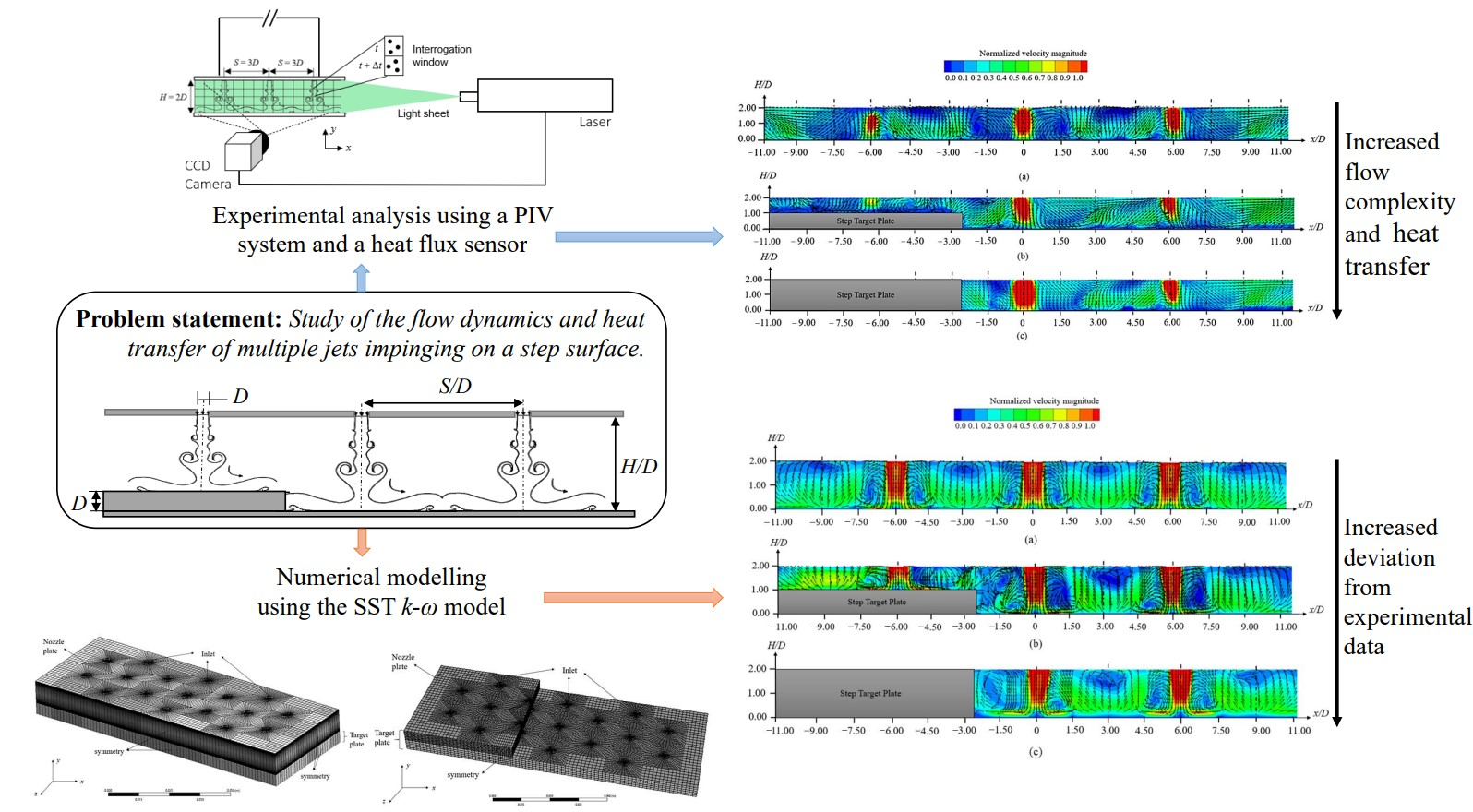
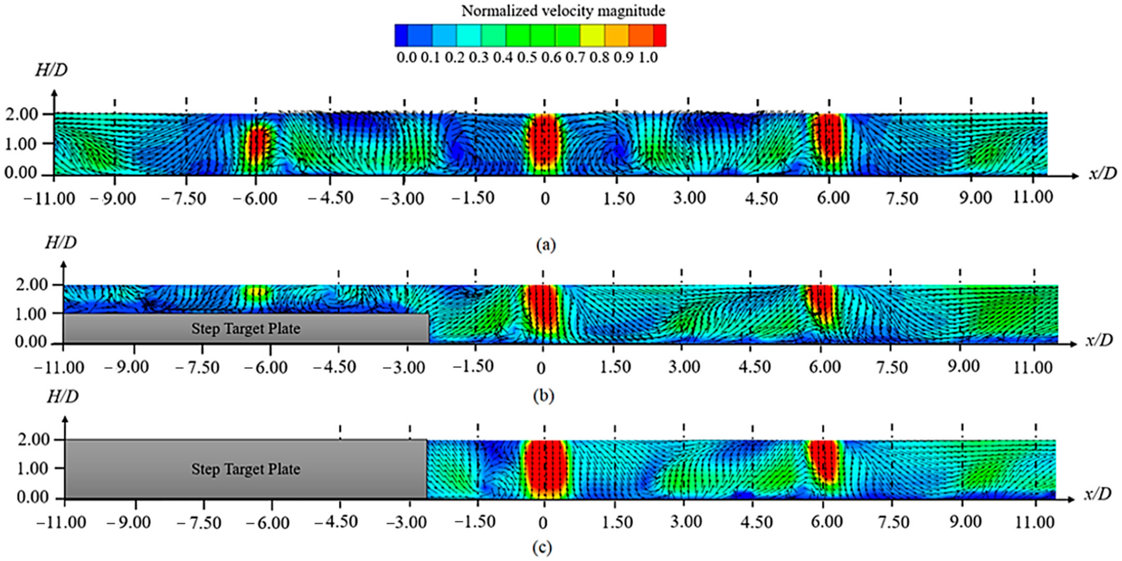
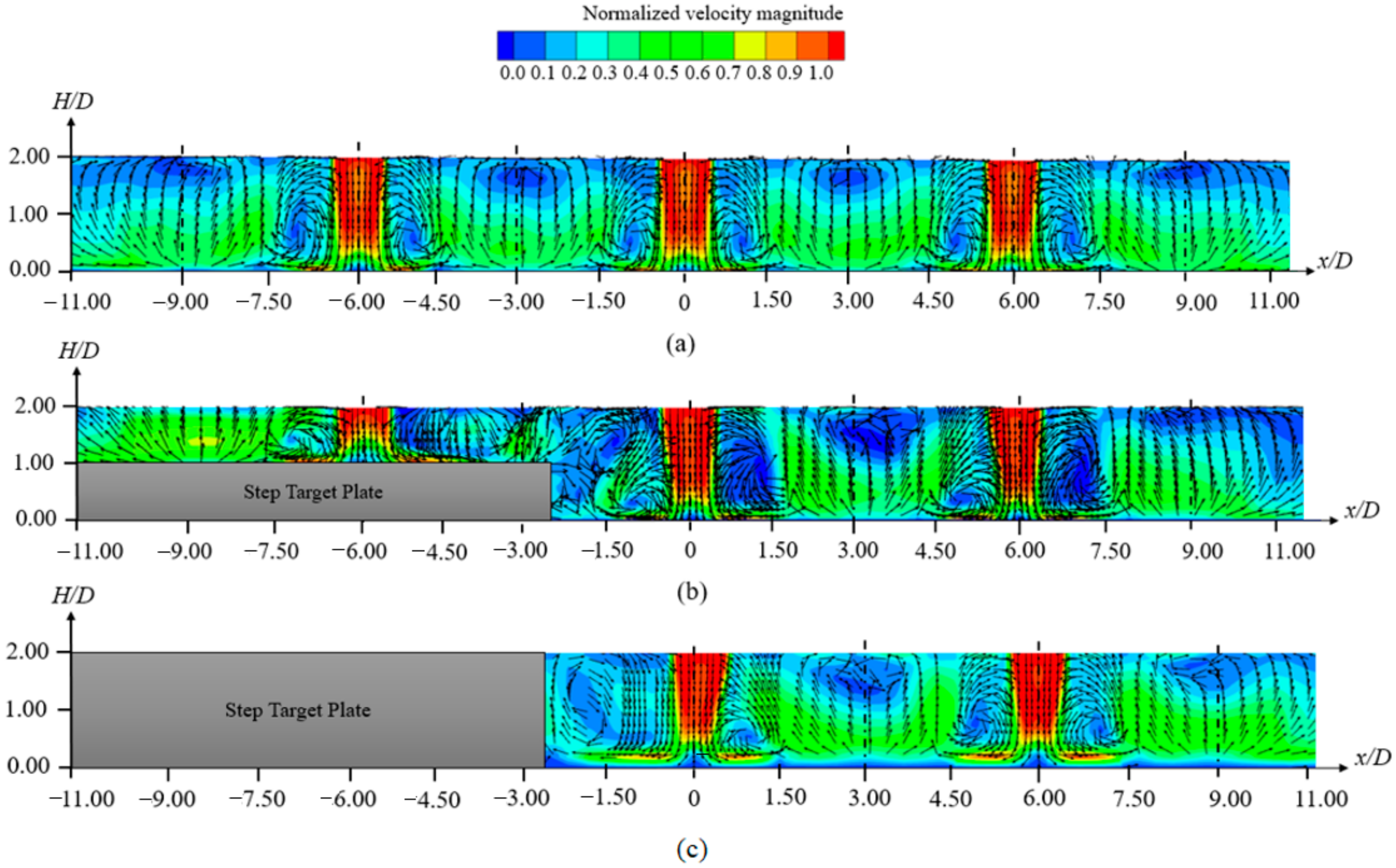
The averaged velocity field of multiple jets impinging on target plates with different configurations was obtained from PIV measurements, and the results are presented in Figure 8. As previously mentioned, the row illuminated by the laser sheet contained the central jet and two adjacent jets, one on each side. However, the effect of the jets located at the front and back rows also had to be quantified due to the staggered configuration. In summary, the multiple jet flow analysis consisted of seven jets. Even if the measuring zone was totally open, the effect of the outlets on the impingement could only be considered on the right and left end side of the impingement plate since a total of nine rows (four on each side of the central row) were considered.
Starting with an overall analysis of the multiple jets’ flow dynamics depicted in Figure 8, it was observed that the air flowed through the circular nozzles at a maximum velocity and started to mix with the surrounding air, entraining mass, momentum, and energy [52]. This is known as the free jet region. From the mixing between the jet flow and the ambient air, a shear layer was generated leading to high lateral velocity gradients. As mentioned by [53], jet impingements characterized by 0.5 < H/D < 5 are within the length of the potential core. This means that no decaying or fully developed regions were expected to be identified. As the jets approached the wall, the axial velocity decreased and was transformed into an accelerated horizontal component [54]. This was identified as the stagnation region, which was characterized by a higher static pressure and a thin boundary layer [55]. The development of the flow over the target plate induced a wall jet region, in which the flow velocity was accelerated along the plate from zero to a maximum at a specific distance from the stagnation point. The jets’ flow was divided into two streams moving in opposite directions, being characterized by a growing boundary layer [56]. Considering this jet flow structure, higher heat transfer coefficients were expected to be recorded in the vicinity of the stagnation region, but a portion of the wall jet region significantly contributed to the heat exchange [57]. However, as presented in Figure 8, the jets’ flow complexity not only was increased by the jets’ interactions upstream and downstream of the impingement but also was increased by the non-flat plate.
Considering that the ratio H/D was small, a high velocity magnitude was identified from the nozzle exit to the target surface. Observing in detail the central jet, results show that the wall jet developed through the surface until it collided with the wall jet of adjacent jets located in the back and front rows. These interactions induced a fountain flow at x/D ≈ ±3 and recirculation regions, identified by Caliskan et al. [58] as primary vortices. The magnitude and structure of these vortices, located on both sides of the central jet axis, seemed to be symmetric in the flat plate case (Figure 8a). As the flow went through the outlets, an increase in the velocity magnitude was observed in direction of the adjacent jets, located at x/D equal to ±6. The interactions between the wall jets induced by the central jet and the adjacent jets located at the front and back rows led to a deflection of the adjacent jets flow located at x/D = ±6. This deflection was mainly due to the development of primary vortices generated at the right end side of the left jet and at the left end side of the right jet, which resulted from wall-jets development and jet-induced crossflow generated by the upstream jets. As mentioned by [55], the self-induced crossflow causes an asymmetric jet flow field, disturbs other wall jets, moves the stagnation points, and develops thicker boundary layers, reducing the average heat transfer rates. This behavior was clearly observed in the three cases presented in Figure 8. Thus, a reduction in the stagnation region of adjacent jets located at x/D = ±6 was verified and a weaker local heat transfer was expected in this region. The second increase in velocity magnitude was observed at x/D ≈ ±9, which represented the position of adjacent jets located at the front and back rows. The increased flow velocity was clear near the outlets, showing the magnitude of the crossflow generated by the upstream jets flow.
Regarding the non-flat plate case, the jet flow dynamics were slightly different. As identified in Figure 8b, the wall jet development induced by the central jet was blocked by the step, inducing a flow reversal. In addition, the step deflected the flow from the adjacent jets located just above the step. The combination of these two effects increased the flow turbulence and affected the central jet flow. The vortex-induced in the left-hand side of the central jet deflected the central jet flow, and the stagnation point was moved to the right side. Even if the primary structure of the central jet was affected, the vortex promoted the mixing, which may have enhanced the heat transfer at the stagnation point [54]. Comparing the two-step configurations, with 1 D (Figure 8b) and 2 D (Figure 8c) heights, the average velocity field shows that the 2 D step blocked the flow generated by the jets located immediately above step, while in the 1 D case, the small gap enabled the development of a short jet over the surface, ensuring its cooling. In that sense, higher velocities were induced in the vicinity of the 2 D step, increasing the overall turbulence of the flow. The deflection of the central jet was weaker when compared with the 1 D step. Therefore, there was no motion of the stagnation point. It was expected that this increased turbulence would enhance the heat transfer rates compared with the flat plate and the 1 D step.
As in the flat plate case, an increased velocity between the central jet and those adjacent, promoted by the jets located at the front and back rows, was identified. As the wall jet induced by the central jet went through the outlet, colliding with the wall jets from the adjacent jets, the deflection of the adjacent jets located at x/D = −6 was observed. This led to a decrease in the impingement area, and a reduced local heat transfer was expected in this region.
Beyond the influence of the target plate configuration, the PIV measurements show that the confined space played an important role in the velocity magnitude. Since the jets’ flow had a reduced space in which to develop, an increase in the flow vorticity was observed. The increase in velocity led to an overall increase in the flow turbulence. Including a step over the target plate, this space became even smaller, which induced a stronger mixing between the multiple jets flow and the surrounding air. In that sense, higher heat transfer rates were expected over a non-flat plate with the configurations presented in this study.

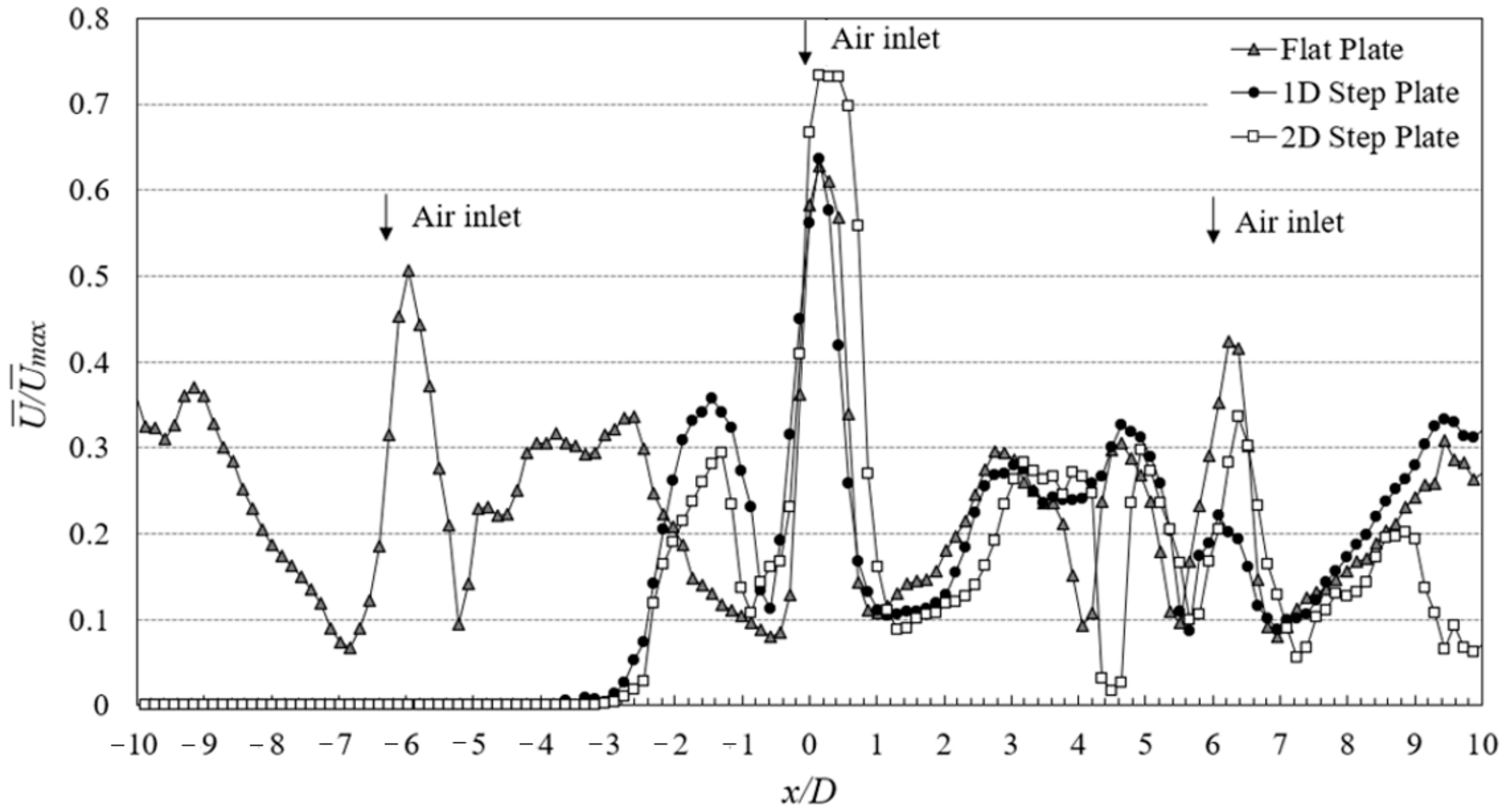
4.2. Velocity Profile over the Target Plate

The velocity profile over the target plate is depicted in Figure 9 for the three plate configurations. To conduct the analysis, the average velocity magnitude was normalized by the maximum velocity (   U ¯ /   U ¯ max), as well as the distance from the central jet axis (x/D).
An overall view of the velocity field over the target plate, depicted in Figure 9, shows that higher velocities were recorded at the beginning of the wall jet development, immediately outward the stagnation region of the central jet in all cases. This flow acceleration was induced after the flow deflection and was characterized by increased shear forces and a thin boundary layer. As previously discussed, the central jet’s flow kept its regular structure while the adjacent jets were affected by the interaction of the upstream jets’ flow. This deflection led to a decrease in the velocity recorded at the adjacent jets’ stagnation zone located at x/D = 6. As expected from the previous analysis, higher velocities were achieved at the acceleration region induced in the vicinity of the stagnation region of the central jet impinging the 2 D step plate. Therefore, higher local heat transfer rates were expected to be recorded. The velocity magnitude over the plate started to decrease as the radial distance (x/D) from the central jet axis increased. This decrease was approximately the same for the three cases, achieving a minimum value at x/D = 1. As the central wall jet developed over the target plate, flow interactions occurred due to the collision with the wall-jet of the adjacent jets. These interactions increased the flow turbulence and consequently an increase in velocity was observed, achieving a secondary peak at x/D ≈ 3. This location corresponds to the vicinity of the stagnation region of adjacent jets located at the front and back rows. As the results demonstrate, the magnitude of the secondary peak was approximately the same for all cases. Near x/D = 4, a decrease in velocity was observed and had to correspond to a stagnation point induced by the collision between the wall jet’s flow. The third velocity peak was identified near the stagnation region of the adjacent jet located at x/D = 6, as expected. Comparing the different cases, it seems that the higher velocity was identified for the flat plate case. This shows that the deflection of the adjacent jet flow was stronger for the non-flat plates, leading to a reduction in the local velocity. As the flow went through the outlet, an increase in flow turbulence was also identified due to the interaction of the upstream jets-induced crossflow with the adjacent jets located at x/D = 9.
Looking at the left-hand side, the velocity profile shows a peak near x/D = −1.5 for the non-flat plate cases. This peak was induced by the increased flow vorticity generated by the collision of the central wall jet with the step surface. This peak is slightly higher for the 1 D step due to the cumulative effect of the deflection of the adjacent jet flow located at x/D = −3 and the step corner with the central wall jet. At the bottom of the step, a stagnation point was identified, recording a velocity near zero. For the case of the flat plate case, a peak was recorded near x/D = −3 due to the strong interactions between the wall jets of the jets positioned in the front and back row with the one located in the central row. Finally, another maximum velocity was observed at x/D = −6, being higher than the one identified at x/D = 6, showing that the magnitude of the vortex that induced the deflection of the adjacent jet (x/D = −6) and that is identified in Figure 8, was lower than the vortex that interfered with the jet located at x/D = 6. These results demonstrate the complexity of the flow field and the difficulty of obtaining uniform development of the flow over the target surface. These effects were stronger when non-flat target plates were applied.

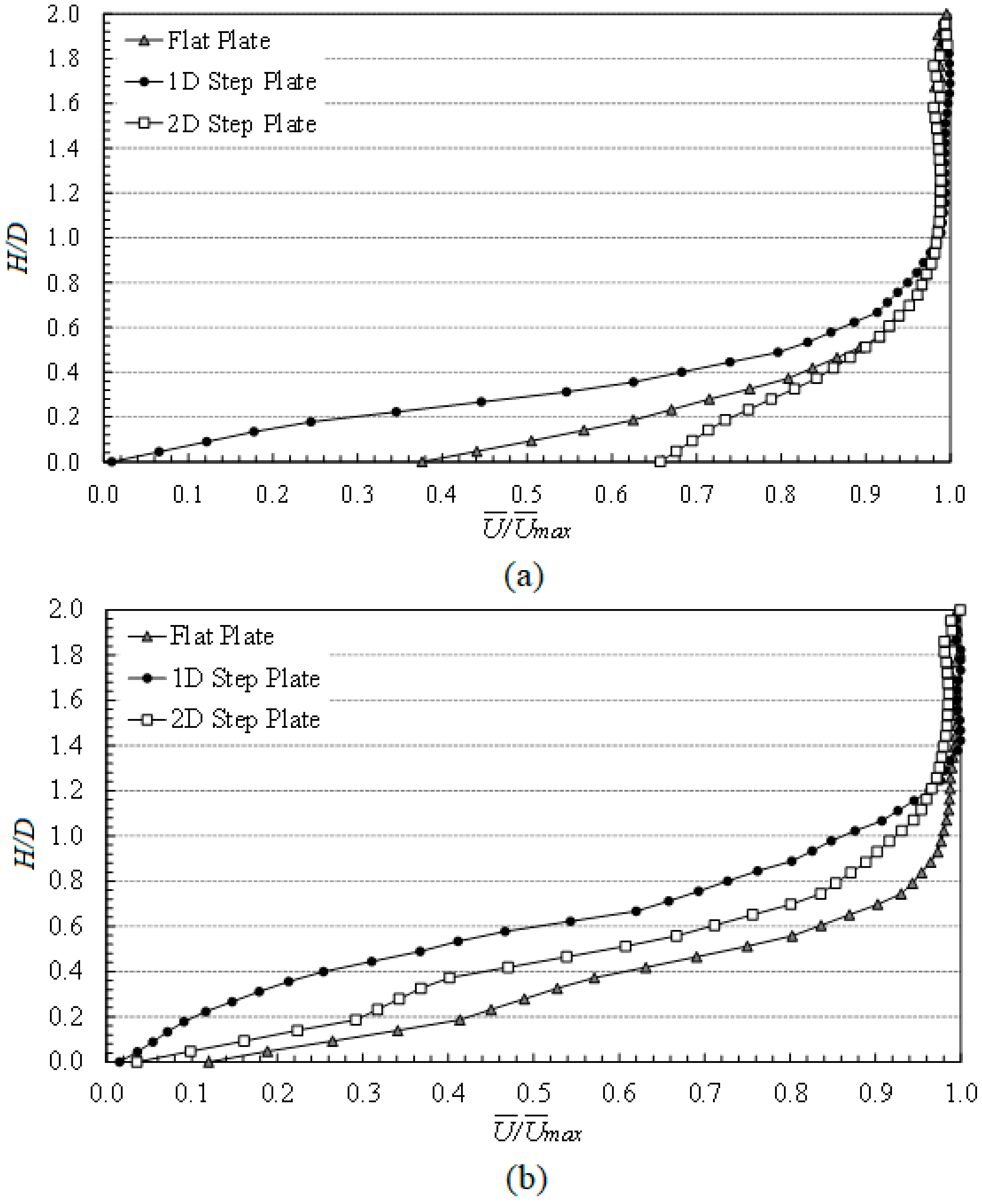
4.3. Velocity Profile over the Central Jet Axis

The velocity profile at the central jet axis and that adjacent on the right are presented in Figure 10a,b, respectively. The velocity profile recorded at the jets’ axis shows the effect of the target plate geometry on the jets’ flow development.
Looking at the central jet, the results demonstrate that near zero velocities at the stagnation point were only identified in the 1 D step plate case, while higher velocities were recorded in the case of the flat plate and 2 D step plate. These results show the limitation of the PIV system to measure, with accuracy, the velocities near the target plate. To improve these measurements and to be able to capture the stagnation points, the CCD camera should focus the flow at the surface transition instead of the overall, from the nozzle to the target plate. While the velocity field recorded by the PIV system and presented in Figure 8 does not allow clear identification of the different jets’ regions, the velocity profile at the jet axis (Figure 10) shows that 95% of the maximum velocity, the end of the potential core, was achieved at H/D near 0.7 for the flat and 2 D step plates and 0.8 for the 1 D step plate. These data demonstrate that the 1 D step induced higher fluctuations of the flow, due to the jets’ flow separation near the step. The vortex previously identified in Figure 8, highly contributed to this reduction in the potential core length compared with the other cases. These interactions were not observed in the 2 D step case since the step height was similar to the nozzle-to-plate separation. Comparing these values with those obtained at the axis of the adjacent jets, the data show a reduction in the actual length of the potential core. A decrease of 20% was identified in the flat plate case, and 40% and 65% for the 2 D step and 1 D step cases, respectively. These results evidence not only that the adjacent jets were strongly affected by the upstream jets but also that the non-flat plate increased the flow turbulence. The higher decrease was identified in the 1 D step configuration, as expected. The end of the potential core indicates the beginning of the stagnation region that extended from H/D near 0.8 to H/D = 0.
Considering that the distance between the nozzle and the target plates was small (H/D = 2), other jet regions identified by [57], such as the decaying and acceleration regions, were not observed in the central jet. However, this was not the case for the adjacent jets. The reduction in the potential core length, as described above, was mainly due to the increased magnitude of the primary vortices. The intensity of the flow turbulence increased with more complex surfaces, and a gradual acceleration between the end of the potential core and the stagnation region was observed. In addition, while velocities near zero at the stagnation point were not detected in all central jets, this was not the case for the adjacent jets.

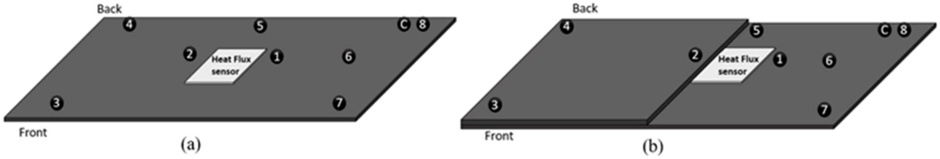
4.4. Average Heat Transfer over a Flat and Non-Flat Plate

The average heat transfer of multiple air jets impinging a flat and non-flat plate is analyzed in this section. The average Nusselt numbers obtained from the heat flux measurements for the flat and non-flat plate cases are summarized in Table 3, as well as the uncertainty of the measurements.
The results demonstrate that the heat transfer was increased by the non-flat plate. These observations are in agreement with the velocity profiles obtained in the previous sections. Compared with the flat plate, the heat transfer increased about 10% for the case of the 1 D step plate and 20% for the 2 D step plate. As mentioned previously, the step surface increased the turbulence inside the confined space between the nozzle and the target plates. As a consequence, higher velocities were measured by the PIV system compared with the flat plate. This increased turbulence promoted the mixing between the jets’ flow and the surrounding air, increasing the heat transfer. In addition to the overall increase in the flow turbulence, the step induced a deflection of the jets that directly impinged over it and blocked the wall jet development coming from the central jet, inducing a flow recirculation. This phenomenon increased the local heat transfer, which was also observed by others [10]. This observation can be explained by the larger stagnation zone of the central jet compared with the other cases, which induced higher heat transfer rates. According to [59], the heat transfer mechanism in the stagnation region is caused by the dynamic behavior of recirculation zones characterized by stagnant heated fluid and the sweeping of the heated fluid. Thus, these circulation zones were expected to be identified with a stronger intensity in the 2 D step plate. To support these conclusions, more analysis with smaller step dimensions is needed.

5. Numerical Model Validation

To evaluate the accuracy of the numerical model for the case of a flat plate, the average Nusselt number obtained numerically was compared with correlations developed by [60,61] and expressed in Equations (17) and (18), respectively.
Nu ¯ = A Re m { 1 B [ ( H / D ) ( U c f / U j ) ] n } Pr 1 / 3
Nu ¯ = 0.328 Re 0.8 ( H / D ) a A f 0.595
where Pr is the Prandtl number, and Af is the free area determined by the ratio between the total nozzle exit area and the total target area. The coefficients A, B, m, and n are defined in [60], while a is described in [61].
The results for Nu ¯ , summarized in Table 4, show that the numerical predictions present a maximum deviation of 12% when compared with the correlations, which seems to be reasonable, according to other studies [44,54,62,63]. When compared with the experimental data, this difference is approximately equal to 5%, which is an acceptable difference, explained by external factors that are not accounted for numerically. Therefore, the numerical model was validated.
Regarding the step plate, numerical and experimental results for the average Nusselt number are presented in Table 5. Compared with the experimental data, a difference of 5% and 15% is observed for the 1 D and 2 D step plate cases, respectively. These results show that, as the complexity of the flow increased, the difference between experimental and numerical data also increased. To analyze the effects that led to this difference, the velocity fields obtained numerically are presented in Figure 11 and compared with the experimental results.
Starting with the analysis of the flat plate case, Figure 11a, the numerical velocity fields present a steady structure, with a symmetric vortex on both sides of the jets; a fountain flow was identified between each jet, located at x/D equal to ±3 and ±9, as expected. However, although this is the profile expected, the experimental results presented in Figure 8 show a more unsteady structure, in which the adjacent jets were more affected by the wall jets and jet-induced crossflow. This led to a deflection of the jets and breakdown of the primary vortices structure. This unpredictability of the flow made it difficult to obtain a velocity profile that matched exactly with those obtained experimentally.
Increasing the complexity of the domain, the results show that the 1 D step highly interfered with the jets’ flow structure compared with the flat and the 2 D step plates. The impingement of the jets located in the front and back rows, and positioned at x/D = ±3, led to a complex flow behavior, clearly identified by the velocity vectors, and the structure of the vortex generated near the step by the central jet was destroyed, as shown in Figure 11b. Due to this effect, the boundary layer located at the left-hand side of the central jet was reduced, compared with the 2 D step plate; therefore, a reduction in the heat transfer was expected compared with this case. The complex flow structure near the step interfered with the global flow development over the domain. Looking at the adjacent jet located on the right-hand side, the results show that, while in the flat and the 2 D plate cases the vortices induced in both sides of the jet were approximately symmetric, this was not the case for the 1 D step. The magnitude of the vortex induced on the left-hand side was stronger, leading to a slight deflection of the jets. These observations are in agreement with the experimental results. Looking at the left-hand side adjacent jet, the numerical results predict with accuracy the jet flow development, a detail that was not captured experimentally. The optical interaction between the laser sheet and the step produced a shadow that decreased the accuracy of the PIV measurements, showing once again the necessity for improving the measurements in the vicinity of the wall. Over the step, due to the reduction in the space between the nozzle and the target plates, an increase in the flow velocity was observed on the left hand-side of the adjacent jet. This can lead to a non-uniform cooling of the step surface.
Focusing on the 2 D step, the numerical results (Figure 11c) are slightly different than the experimental ones (Figure 8c), mainly near the step. The perfect roll up structure induced by the central jet was not captured experimentally. In contrast, it seems that a combination between the staggered configuration and the 2 D step led to an increase in velocity magnitude near the step, which was not identified numerically. This effect induced an increase in the heat transfer, which explains the difference between numerical and experimental results expressed in Table 5. While a typical jet flow structure is presented by the numerical model, the experimental results clearly show that as the complexity of the domain increased, the jets’ flow structure became more unstable, and this was difficult to predict numerically, as previously mentioned. However, this tool is important and provides interesting results for a global analysis of the flow. As stated by several authors [44,54,62,63], a deviation between the numerical and experimental results close to 10% is acceptable. In addition, looking at the stagnation region of the central jet, it seems to have been slightly thinner compared with the experimental results. Looking at the development of the primary vortices on both sides of the jet axis, this difference can be explained by the slight deviation of the central jet flow due to the strong interference of the vortex located on the left-hand side. Therefore, a reduction in the local heat transfer was expected. Moreover, at the bottom of the step, a stagnation point was identified both numerically and experimentally, which could induce a hot spot. The effect of the symmetry boundary conditions was reflected close to the right-hand side of the domain and did not reflect with accuracy the effect of the jet-induced crossflow, which increased from the central jet to the outlets. This observation is also valid for the flat plate case. In that sense, this can be a parameter to improve in future simulations, and a lower divergence between numerical and experimental results is expected to occur.
To conclude, an overall analysis of the numerical results shows that the SST k-ω model provided accurate predictions of the jet flow dynamics of multiple jets impinging on a flat and non-flat surface. The vortices induced in the vicinity of the step plate were captured with high detail, as was the deflection of the flow field due to the step corner. The higher resolution of the numerical results provides a better identification of the stagnation when compared with the experimental data. The PIV setup needs to be improved in the vicinity of the wall. Although the instability of the flow was difficult to predict numerically, leading to a reduced deflection of the jets’ flow and a weaker influence of the jet-induced crossflow compared with the experiments, this difference resulted in a low discrepancy between numerical and experimental average heat transfer values. Therefore, this model can be implemented to predict the jet flow dynamics and heat transfer of multiple jet impingement processes.

6. Conclusions

This work presents the flow dynamics and average heat transfer of multiple jets impinging flat and non-flat surfaces. Through PIV measurements, velocity fields were obtained and compared. The analysis of the overall flow field shows that combining the staggered configuration with the confinement induced stronger interference of upstream jet-induced crossflow on downstream jets, slightly increasing the heat transfer over the impinging surface. This effect was intensified in the non-flat plates due to the reduction in the overall area by the step. The velocity profiles over the jets’ axes were extracted from the post-processed PIV data and allowed detailed analysis of the variation of the velocity magnitude. In that sense, the different jet regions were detected and the influence of the plate geometry and jets interactions on the flow development over the target plate was analyzed. The results demonstrate the complexity of the flow due to adjacent jets interactions, which were intensified by the non-flat plate. The step induced a flow reversal of the central wall jet. This effect, combined with the jets’ interactions, led to an increase in the velocity magnitude in the vicinity of the step. Compared with the flat plate, the average heat transfer increases about 10% for the case of the 1 D step plate and 20% for the 2 D step plate. The higher heat transfer value must be explained by the fact that the central jet of the 2 D step plate presented a larger stagnation region. However, to support these conclusions, more analysis with smaller step dimensions is needed. Regarding the numerical model, results show good accuracy of the average heat transfer for the case of the flat and the 1 D step plate, with a difference of 5% compared with the experimental results. These results show the potential of this turbulence model to predict the influence of the plate roughness effect, which is in agreement with [11], even for higher Reynolds numbers. Even if the velocity field predicted numerically did not correspond exactly with the PIV measurement, it seems that the effects on the average heat transfer were reduced. However, this was not the case for the 2 D step plate since a difference of 15% was identified. Looking at the velocity field obtained numerically, it seems that this higher difference was due to the difficulty of predicting with accuracy the jet flow structure due to the strong unsteadiness of the flow as the complexity of the domain was increased. Therefore, improvements to the model are needed for this more complex case. Overall, the SST k-ω model seems to be a suitable solution for predicting jets’ flow and heat transfer over a non-flat surface.

Author Contributions

Conceptualization, J.C.F.T. and S.F.C.F.T.; methodology, software, validation, formal analysis, and investigation, F.V.B.; resources, J.C.F.T. and S.F.C.F.T.; writing—original draft preparation, F.V.B.; writing—review and editing, J.C.F.T. and S.F.C.F.T.; supervision, J.C.F.T. and S.F.C.F.T.; project administration, J.C.F.T. All authors have read and agreed to the published version of the manuscript.

Funding

This research received no external funding.

Acknowledgments

The first author would like to express her gratitude for the support given by the Portuguese Foundation for Science and Technology (FCT) and the MIT Portugal Program. This work was supported by FCT—Fundação para a Ciência e Tecnologia within the R&D Units Project Scope: UIDB/00319/2020 (ALGORITMI Center) and Project Scope UIDB/00319/2020 (METRICS Center).

Conflicts of Interest

The authors declare no conflict of interest. The funders had no role in the design of the study; in the collection, analyses, or interpretation of data; in the writing of the manuscript; or in the decision to publish the results.

Nomenclature

SymbolQuantitySI Unit
AfNon-dimensional area-
DDiameter(m)
DωCross-diffusion term-
DkGeneration of k(kg/m·s3)
GωGeneration of ω(kg/m3·s2)
hHeat transfer coefficient(W/m2K)
HNozzle-to-plate distance(m)
kTurbulent kinetic energy; Thermal conductivity(m2/s2); (W/mK)
kpExpansion factor-
NSamples number-
Nu ¯ Average Nusselt number-
pPressure(Pa)
  q ¯ Average heat flux(W/m2)
ReReynolds number-
SJet-to-jet spacing(m)
Sk, SωSource term(W/m3)
tTime(s)
TTemperature(°C)
uUncertainty/velocity(dependent variable)/(m/s)
  U ¯ Average velocity(m/s)
y + Dimensionless distance of the first node to the wall-
x, y, zCartesian coordinates-
u, v, wVelocity according to the Cartesian coordinates(m/s)
Greek Symbol
Γ k ,   Γ ω Effective diffusivity of k, ω(kg/m·s)
ΔSMagnification factor
ΔxThickness(m)
ΔxpParticle’s displacement(m)
εRandom error(dependent variable)
κThermal diffusivity(m2/s)
μDynamic viscosity(Pa/s)
ρDensity(kg/m3)
σStandard deviation-
ωSpecific dissipation rate(1/s)
Subscript
Ambient air
cfCrossflow
jJet
maxMaximum
wWall

References

  1. Intelligence, M. Printed Circuit Board Market-Growth, Trends, Forecasts (2020–2025); Mordor Intelligence: Hyderabad, India, 2020. [Google Scholar]
  2. Lau, C.-S.; Abdullah, M.; Ani, F.C. Three-dimensional thermal investigations at board level in a reflow oven using thermal-coupling method. Solder. Surf. Mt. Technol. 2012, 24, 167–182. [Google Scholar] [CrossRef]
  3. Whalley, D.C. A simplified model of the reflow soldering process. J. Mater. Process. Technol. 2004, 150, 134–144. [Google Scholar] [CrossRef]
  4. Balázs, I.; Harsányi, G. Heating characteristics of convection reflow ovens. Appl. Therm. Eng. 2009, 29, 2166–2171. [Google Scholar]
  5. Tsai, T.-N. Thermal parameters optimization of a reflow soldering profile in printed circuit board assembly: A comparative study. Appl. Soft Comput. 2012, 12, 2601–2613. [Google Scholar] [CrossRef]
  6. Caliskan, S.; Baskaya, S. Experimental investigation of impinging jet array heat transfer from a surface with V-shaped and convergent-divergent ribs. Int. J. Therm. Sci. 2012, 59, 234–246. [Google Scholar] [CrossRef]
  7. Chauhan, R.; Thakur, N. Heat transfer and friction factor correlations for impinging jet solar air heater. Exp. Therm. Fluid Sci. 2013, 44, 760–767. [Google Scholar] [CrossRef]
  8. Nayak, R.; Singh, S. Effect of geometrical aspects on the performance of jet plate solar air heater. Sol. Energy 2016, 137, 434–440. [Google Scholar] [CrossRef]
  9. Buzzard, W.C.; Ren, Z.; Ligrani, P.M.; Nakamata, C.; Ueguchi, S. Influences of target surface small-scale rectangle roughness on impingement jet array heat transfer. Int. J. Heat Mass Transf. 2017, 110, 805–816. [Google Scholar] [CrossRef]
  10. Alenezi, A.H.; Almutairi, A.; Alhajeri, H.M.; Addali, A.; Gamil, A.A.A. Flow Structure and Heat Transfer of Jet Impingement on a Rib-Roughened Flat Plate. Energies 2018, 11, 1550. [Google Scholar] [CrossRef] [Green Version]
  11. Tepe, A.Ü.; Uysal, Ü.; Yetişken, Y.; Arslan, K. Jet impingement cooling on a rib-roughened surface using extended jet holes. Appl. Therm. Eng. 2020, 178, 115601. [Google Scholar] [CrossRef]
  12. Lo, Y.-H.; Liu, Y.-H. Heat transfer of impinging jet arrays onto half-smooth, half-rough target surfaces. Appl. Therm. Eng. 2018, 128, 79–91. [Google Scholar] [CrossRef]
  13. Nadda, R.; Kumar, R.; Kumar, A.; Maithani, R. Optimization of single arc protrusion ribs parameters in solar air heater with impinging air jets based upon PSI approach. Therm. Sci. Eng. Prog. 2018, 7, 146–154. [Google Scholar] [CrossRef]
  14. Ren, Z.; Yang, X.; Lu, X.; Li, X.; Ren, J. Experimental Investigation of Micro Cooling Units on Impingement Jet Array Flow Pressure Loss and Heat Transfer Characteristics. Energies 2021, 14, 4757. [Google Scholar] [CrossRef]
  15. Nagesha, K.; Srinivasan, K.; Sundararajan, T. Enhancement of jet impingement heat transfer using surface roughness elements at different heat inputs. Exp. Therm. Fluid Sci. 2020, 112, 109995. [Google Scholar] [CrossRef]
  16. De Oliveira, M.A.; De Moraes, P.G.; De Andrade, C.L.; Bimbato, A.M.; Pereira, L.A.A. Control and Suppression of Vortex Shedding from a Slightly Rough Circular Cylinder by a Discrete Vortex Method. Energies 2020, 13, 4481. [Google Scholar] [CrossRef]
  17. Slama, M.; Bex, C.C.; Pinon, G.; Togneri, M.; Evans, I. Lagrangian Vortex Computations of a Four Tidal Turbine Array: An Example Based on the Nepthyd Layout in the Alderney Race. Energies 2021, 14, 3826. [Google Scholar] [CrossRef]
  18. Spring, S.; Xing, Y.; Weigand, B. An Experimental and Numerical Study of Heat Transfer From Arrays of Impinging Jets with Surface Ribs. J. Heat Transf. 2012, 134, 082201. [Google Scholar] [CrossRef]
  19. Casanova, J.O.; Granados-Ortiz, F. Numerical simulation of the heat transfer from a heated plate with surface variations to an impinging jet. Int. J. Heat Mass Transf. 2014, 76, 128–143. [Google Scholar] [CrossRef]
  20. Brakmann, R.; Chen, L.; Weigand, B.; Crawford, M. Experimental and Numerical Heat Transfer Investigation of an Impinging Jet Array on a Target Plate Roughened by Cubic Micro Pin Fins1. J. Turbomach. 2016, 138, 111010. [Google Scholar] [CrossRef]
  21. Shukla, A.K.; Dewan, A. Convective Heat Transfer Enhancement using Slot Jet Impingement on a Convective Heat Transfer Enhancement using Slot Jet Impingement on a Detached Rib Surface. J. Appl. Fluid Mech. 2017, 10, 1615–1627. [Google Scholar]
  22. Jing, Q.; Zhang, D.; Xie, Y. Numerical investigations of impingement cooling performance on flat and non-flat targets with dimple/protrusion and triangular rib. Int. J. Heat Mass Transf. 2018, 126, 169–190. [Google Scholar] [CrossRef]
  23. McInturff, P.; Suzuki, M.; Ligrani, P.; Nakamata, C.; Lee, D.H. Effects of hole shape on impingement jet array heat transfer with small-scale, target surface triangle roughness. Int. J. Heat Mass Transf. 2018, 127, 585–597. [Google Scholar] [CrossRef]
  24. Chen, L.; Brakmann, R.G.; Weigand, B.; Poser, R.; Yang, Q. Detailed investigation of staggered jet impingement array cooling performance with cubic micro pin fin roughened target plate. Appl. Therm. Eng. 2020, 171, 115095. [Google Scholar] [CrossRef]
  25. Menter, F.R. Two-equation eddy-viscosity turbulence models for engineering applications. AIAA J. 1994, 32, 1598–1605. [Google Scholar] [CrossRef] [Green Version]
  26. Melling, A. Tracer particles and seeding for particle image velocimetry. Meas. Sci. Technol. 1997, 8, 1406–1416. [Google Scholar] [CrossRef]
  27. Keane, R.D.; Adrian, R.J. Theory of cross-correlation analysis of PIV images. Appl. Sci. Res. 1992, 49, 191–215. [Google Scholar] [CrossRef]
  28. Westerweel, J. Fundamentals of digital particle image velocimetry. Meas. Sci. Technol. 1997, 8, 1379–1392. [Google Scholar] [CrossRef] [Green Version]
  29. Zhang, C.; Vasilevskis, S.; Kozlowski, B. Particle Image Velocimetry-User Guide; Department of Civil Engineering, Aalborg University: Aalborg, Denmark, 2018. [Google Scholar]
  30. Cao, X.; Liu, J.; Jiang, N.; Chen, Q. Particle image velocimetry measurement of indoor airflow field: A review of the technologies and applications. Energy Build. 2014, 69, 367–380. [Google Scholar] [CrossRef] [Green Version]
  31. Childs, P.R.N.; Greenwood, J.R.; Long, C.A. Heat flux measurement techniques. Proc. Inst. Mech. Eng. Part C 1999, 213, 655–677. [Google Scholar] [CrossRef]
  32. Assaad, M.C.; Kimble, B.; Huang, Y.-M.; Burgan, R.; Fralick, G.C.; Wrbanek, J.D.; Gonzalez, J.M. Thin-Film Heat Flux Sensor for Measuring the Film Coefficient of Rubber Components of a Rolling Tire. Tire Sci. Technol. 2008, 36, 275–289. [Google Scholar] [CrossRef]
  33. Cengel, Y.A.; Ghajar, A.J. Heat and Mass Transfer: Fundamentals and Applications, 5th ed.; McGraw-Hill Education: New York, NY, USA, 2011. [Google Scholar]
  34. Sabharwall, P.; Conder, T.; Skifton, R.; Stoots, C.; Kim, E.S. PIV Uncertainty Methodologies for CFD Code Validation at the MIR Facility; Idaho National Laboratory: Idaho Falls, ID, USA, 2013. [Google Scholar]
  35. Sciacchitano, A. Uncertainty quantification in particle image velocimetry. Meas. Sci. Technol. 2019, 30, 092001. [Google Scholar] [CrossRef] [Green Version]
  36. Barbosa, F.; Costa, C.; Teixeira, S.; Teixeira, J.C. Measurement Errors and Uncertainty Quantification of a 2D-PIV Experimental Setup for Jet Flow Characterization. ASCE-ASME J. Risk Uncertain. Eng. Syst. Part B Mech. Eng. 2020, 6, 1–59. [Google Scholar]
  37. Dantec Dynamics. Dynamic Studio, User’s Guide; Dantec Dynamics: Skovlunde, Denmark, 2016. [Google Scholar]
  38. ASME. Test. Uncertainty. Instruments and Appartus; The American Society of Mechanical Engineers: New York, NY, USA, 1998. [Google Scholar]
  39. Sciacchitano, A.; Wieneke, B. PIV uncertainty propagation. Meas. Sci. Technol. 2016, 27, 84006. [Google Scholar] [CrossRef] [Green Version]
  40. JCGM. Evaluation of Measurement Data—Guide to the Expression of Uncertainty in Measurement; Joint Committee for Guides in Metrology: Sèvres, France, 2008. [Google Scholar]
  41. ANSYS. Ansys Fluent Theory Guide; ANSYS: Canonsburg, PA, USA, 2013. [Google Scholar]
  42. Zhu, K.; Yu, P.; Yuan, N.; Ding, J. Transient heat transfer characteristics of array-jet impingement on high-temperature flat plate at low jet-to-plate distances. Int. J. Heat Mass Transf. 2018, 127, 413–425. [Google Scholar] [CrossRef]
  43. Barbosa, F.V.; Silva, J.P.V.; Teixeira, S.F.C.; Soares, D.F.; Santos, D.N.F.; Delgado, I.A.C.; Teixeira, J.C.F. Cfd Prediction of Multiple Jet Impingement in a Reflow Soldering Process. In Transactions on Engineering Technologies. WCE 2018; Ao, S.I., Gelman, L., Kim, H.K., Eds.; Springer: Singapore, 2019. [Google Scholar]
  44. Debnath, S.; Khan, H.U.; Ahmed, Z.U. Turbulent swirling impinging jet arrays: A numerical study on fluid flow and heat transfer. Therm. Sci. Eng. Prog. 2020, 19, 100580. [Google Scholar] [CrossRef]
  45. Tepe, A.Ü.; Yetişken, Y.; Uysal, Ü.; Arslan, K. Experimental and numerical investigation of jet impingement cooling using extended jet holes. Int. J. Heat Mass Transf. 2020, 158, 119945. [Google Scholar] [CrossRef]
  46. Shah, S. Numerical analysis of heat transfer between multiple jets and flat moving surface. Int. J. Heat Mass Transf. 2021, 171, 121088. [Google Scholar] [CrossRef]
  47. Menter, F.R.; Ferreira, J.C.; Esch, T. The SST Turbulence Model with Improved Wall Treatment for Heat Transfer Predictions in Gas Turbines. In Proceedings of the International Gas Turbine Congress, Tokyo, Japan, 2–7 November 2003; pp. 1–7. [Google Scholar]
  48. Wen, Z.-X.; He, Y.-L.; Cao, X.-W.; Yan, C. Numerical study of impinging jets heat transfer with different nozzle geometries and arrangements for a ground fast cooling simulation device. Int. J. Heat Mass Transf. 2016, 95, 321–335. [Google Scholar] [CrossRef]
  49. Rhie, C.M.; Chow, W.L. Numerical Study of the Turbulent Flow past an Airfoil with Trailing Edge Separation. AIAA J. 1983, 21, 1525–1532. [Google Scholar] [CrossRef]
  50. Ferziger, J.H.; Peric, M. Computational Methods for Fluid Dynamics, 3rd ed.; Springer: New York, NY, USA, 1996. [Google Scholar]
  51. Lee, J.; Lee, S. Stagnation Region Heat Transfer of a Turbulent Axisymmetric Jet Impingement. Exp. Heat Transf. 2010, 12, 137–156. [Google Scholar] [CrossRef]
  52. Viskanta, R. Nusselt-Reynolds Prize Paper-Heat Transfer to Impinging Isothermal Gas and Flame Jets. Exp. Therm. Fluid Sci. 1993, 6, 111–134. [Google Scholar] [CrossRef]
  53. Barbosa, F.; Teixeira, S.; Teixeira, J. Experimental and numerical analysis of the influence of the nozzle-to-plate distance in a jet impingement process. Int. J. Thermodyn. 2020, 23, 81–91. [Google Scholar] [CrossRef]
  54. Weigand, B.; Spring, S. Multiple Jet Impingement-A Review. Heat Transf. Res. 2011, 42, 101–142. [Google Scholar] [CrossRef]
  55. Zuckerman, N.; Lior, N. Jet Impingement Heat Transfer: Physics, Correlations, and Numerical Modeling. Adv. Heat Transf. 2006, 39, 565–631. [Google Scholar]
  56. Kalifa, R.B.; Habli, S.; Saïd, N.M.; Bournot, H.; le Palec, G. Parametric analysis of a round jet impingement on a heated plate. Int. J. Heat Fluid Flow 2016, 57, 11–23. [Google Scholar] [CrossRef]
  57. Angioletti, M.; Di Tommaso, R.; Nino, E.; Ruocco, G. Simultaneous visualization of flow field and evaluation of local heat transfer by transitional impinging jets. Int. J. Heat Mass Transf. 2003, 46, 1703–1713. [Google Scholar] [CrossRef]
  58. Caliskan, S.; Baskaya, S.; Calisir, T. Experimental and numerical investigation of geometry effects on multiple impinging air jets. Int. J. Heat Mass Transf. 2014, 75, 685–703. [Google Scholar] [CrossRef]
  59. Nozaki, A.; Igarashi, Y.; Hishida, K. Heat transfer mechanism of a swirling impinging jet in a stagnation region. Heat Transf.-Asian Res. 2003, 32, 663–673. [Google Scholar] [CrossRef]
  60. Florschuetz, L.W.; Metzger, D.E.; Takeuchi, D.I.; Berry, R.A. Multiple Jet Impingement Heat Transfer Characteristic—Experimental Investigation of in-Line and Staggered Arrays with Crossflow. NASA Contract. Rep. 1980, 3217, 84. [Google Scholar]
  61. Obot, N.T.; Trabold, T. Impingement Heat Transfer Within Arrays of Circular Jets: Part 1—Effects of Minimum, Intermediate, and Complete Crossflow for Small and Large Spacings. J. Heat Transf. 1987, 109, 872–879. [Google Scholar] [CrossRef]
  62. Chitsazan, A.; Glasmacher, B. Numerical Investigation of Heat Transfer and Pressure Force from Multiple Jets Impinging on a Moving Flat Surface. Int. J. Heat Technol. 2020, 38, 601–610. [Google Scholar] [CrossRef]
  63. Badra, J.; Masri, A.R.; Behnia, M. Enhanced Transient Heat Transfer from Arrays of Jets Impinging on a Moving Plate From Arrays of Jets Impinging on a Moving Plate. Heat Transf. Eng. 2013, 34, 361–371. [Google Scholar] [CrossRef]
Figure 1. Experimental apparatus: (a) 3D model; (b) main structure; (c) impinging plate; (d) control equipment. (Reprinted from Flávia V. Barbosa, Sérgio D. T. Sousa, Senhorinha F. C. F. Teixeira, José C. F. Teixeira, Application of Taguchi Method for the Analysis of a Multiple Air Jet Impingement System with and without Target Plate Motion, 176, September 2021, Copyright (2021), with permission from Elsevier).
Energies 14 06659 g001
Figure 2. Target plate configurations: (a) flat plate; (b) non-flat plate. The scheme represents the location of the heat flux and the numbers are the location of thermocouples over the surface for each configuration.
Energies 14 06659 g002
Figure 3. PIV measurement system.
Energies 14 06659 g003
Figure 4. Thin-film heat flux sensor OMEGA® HFS-4.
Energies 14 06659 g004
Figure 5. Jets position in relation to the heat flux sensor. (a) non-flat plate; (b) flat plate.
Energies 14 06659 g005
Figure 6. Physical domain and boundary conditions. (a) Overall domain; (b) non-flat plate.
Energies 14 06659 g006
Figure 7. Mesh sensitivity analysis.
Energies 14 06659 g007
Figure 8. Velocity field measured experimentally of multi-jets impinging a flat and non-flat plate at Re = 5000, H/D = 2, and S/D = 3. (a) Flat plate; (b) non-flat with 1 D step; (c) non-flat with 2 D step.
Energies 14 06659 g008
Figure 9. Velocity profile over the target plate (y/D = 0.15) for different plate geometry.
Energies 14 06659 g009
Figure 10. Velocity profile over the jet axis. (a) Central jet (x/D = 0); (b) right adjacent jet (x/D = 6).
Energies 14 06659 g010
Figure 11. Velocity field obtained numerically of multi-jets impinging a flat and non-flat plate at Re = 5000, H/D = 2, and S/D = 3. (a) Flat plate; (b) non-flat with 1 D step; (c) non-flat with 2 D step.
Energies 14 06659 g011
Table 1. Systematic uncertainties. (Reprinted from Flávia V. Barbosa, Sérgio D. T. Sousa, Senhorinha F. C. F. Teixeira, José C. F. Teixeira, Application of Taguchi Method for the Analysis of a Multiple Air Jet Impingement System with and without Target Plate Motion, 176, September 2021, Copyright (2021), with permission from Elsevier).
SourceMethod of MeasurementUncertainty
Heat FluxHeat flux sensor±0.577 (W/m2)
Nozzle diameter and heat flux sensor areaCaliper±0.011 (mm)
Target and jets temperatureThermocouples type K±0.115 (°C)
Table 2. Properties of the three grids.
GridN° of ElementsMax y+
Coarse387,0723.27
Medium756,0001.69
Fine1,134,0001.64
Table 3. Average Nusselt number measurements.
Plate GeometryAverage Nusselt Number
Flat29.90 ± 0.45
Non-flat—Step 1 D32.72 ± 0.49
Non-flat—Step 2 D37.39 ± 0.56
Table 4. Average Nusselt number over the target flat plate.
Nu ¯ .  
Numerical ResultExperimental DataFlorshuetz et al. [61]Obot and Trebold [62]
28.6529.90 ± 0.4532.6325.55
Table 5. Average Nusselt number over the step plate.
Nu ¯
Target PlateNumerical ResultExperimental Data
1 D step31.3532.72 ± 0.49
2 D step31.6937.39 ± 0.56
Publisher’s Note: MDPI stays neutral with regard to jurisdictional claims in published maps and institutional affiliations.

