Improving Artificial Intelligence Forecasting Models Performance with Data Preprocessing: European Union Allowance Prices Case Study

Abstract

European Union Allowances (EUAs) are rights to emit CO₂ that may be sold or bought by enterprises. They were originally created to try to reduce greenhouse gas emissions, although they have become assets that may be used by financial intermediaries to seek for new business opportunities. Therefore, forecasting the time evolution of their price is very important for agents involved in their selling or buying. Neural Networks, an artificial intelligence paradigm, have been proved to be accurate and reliable tools for time series forecasting, and have been widely used to predict economic and energetic variables; two of them are used in this work, the Multilayer Preceptron (MLP) and the Long Short-Term Memories (LSTM), along with another artificial intelligence algorithm (XGBoost). They are combined with two preprocessing tools, decomposition of the time series into its trend and fluctuation and decomposition into Intrinsic Mode Functions (IMF) by the Empirical Mode Decomposition (EMD). The price prediction is obtained by adding those from each subseries. These two tools are combined with the three forecasting tools to provide 20 future predictions of EUA prices. The best results are provided by MLP-EMD, which is able to achieve a Mean Absolute Percentage Error (MAPE) of 2.91% for the first predicted datum and 5.65% for the twentieth, with a mean value of 4.44%.

1. Introduction

Since the European Union (EU) created the Emission Trading System (EU ETS) in 2005 to combat climate change, it has become one of the cornerstones of the European environmental policy, with strong implications for industrial activities and repercussions that reach all economic and social sectors. Its main goal is to reduce greenhouse gas emission. It is supposed that companies producing carbon emissions must effectively manage associated costs by buying or selling rights to emit CO₂, the so-called European Union Allowances (EUAs). The EU ETS is a cap-and-trade system, which includes only large stationary sources of emissions belonging to the most pollutant industrial sectors of the European economy (power plants, oil refineries, ferrous metallurgy, cement clinker or lime, glass—including glass fiber—ceramic products by firing, and pulp, paper and board).

Companies involved can either use EUAs to compensate their emissions or sell them to others that need them [1]; they are allowed to trade emission allowances freely within the EU, so the system seeks to ensure that overall emissions are reduced, but also that cuts are made by those companies that can achieve the most efficient abatement costs [2,3].

Although the main EUA market goal was to give firms an incentive to move towards a less fossil fuel-intensive production, it also provides a new asset and new business development opportunities for financial intermediaries. Thus, current allowance prices, as well as the predicted EUA prices, are critical for companies, brokers, traders, and investors, and they can also affect decarbonization investment decisions [4,5,6,7]. Therefore, it may be stated that, although the market is designed to encourage decarbonization investments in the industrial sectors subject to the system, the consideration of emission allowances as financial assets introduces a new component that may complicate the market’s effectiveness in environmental terms.

Regarding the consideration of EUA as financial assets, it would be helpful to obtain short-term reliable forecasts, since agents involved in this market need to make quick buying and selling decisions in order to obtain maximum profitability [8].

However, in terms of the environmental component underlying the market, agents involved in the decisions need to use a longer time horizon. For the system to work properly, the EUA market must provide information that incentivizes decarbonization decisions, even though investments in technological improvements or fuel substitution can take long payback periods. Therefore, incentives for decarbonization decisions must be credible and long-lasting, so that, rather than the information contained in the day-to-day fluctuation of prices, it is the trend of EUA prices that is of interest. In order to favor market stability and fulfillment of the objective of incentivizing decarbonization decisions by maintaining EUA prices, in 2019 the EU created a mechanism—the Market Stability Reserve (MSR)—with the aim of removing the excess of emission allowances that had generated the crisis since 2008. The MSR was designed to absorb excess EUAs in the short-term and to match the supply of EUAs in case of severe shortages in the long-term. However, EUA prices have risen sharply in the last years and this increase can hardly be explained by the purchasing needs of the companies included in the system, but rather by the arrival of other investors in the market, outside the polluting sectors, which are governed by objectives other than those initially set out in the EU ETS. In this case, we are talking about the behavior of EUAs as financial assets, whose price has shown not only rapid growth but also high volatility in the short-term.

The evolution of EUA prices has complicated the current economic situation, as their sharp rise has affected the costs of various sectors, causing significant increases in electricity prices. For example, the wholesale electricity market prices in Spain in September 2021 are three times higher than the year before. Although the cost of EUAs is not the only factor responsible for this price increase, according to some estimates [9], in the case of Spain, around 20% of this increase would be related to the rise of CO₂ prices in the EU ETS. Other European markets have experienced an evolution of wholesale electricity prices very similar to the Spanish one. In this way, the energy price increase in Europe has become macroeconomically significant [10]. Several factors, in addition to the CO₂ rising trend, are responsible for the rise of electricity prices: an increase of natural gas demand forced by higher demand of electric energy along with a decrease in renewable electricity production and a significant increase in coal prices. The pricing system in European (and other) electricity markets assumes that the price of electricity reflects the marginal production cost of the most expensive technology involved in generation. Therefore, fossil fuel power producers incorporate the price of EUAs into the marginal cost, passing on CO₂ prices into electricity prices and, where appropriate, incentivizing investment in renewable sources. The maintenance of high EUAs prices, although may be compatible with the environmental objective of the system and reinforce the incentives for decarbonization, can also lead to problems derived from the increase in costs in all sectors, including the loss of commercial competitiveness in Europe. In addition, the effects of higher electricity prices on consumers can be very significant, affecting different social classes in different ways. Therefore, prediction of the time evolution of EUA prices has become a fundamental tool for enterprises dealing with them, both for the short-term, to manage their day-to-day evolution—linked to its behavior as a financial asset—and the long-term, related to investments and decisions aimed at reducing the emission of greenhouse gases.

Prediction of EAU prices can be carried out by organizing them as times series so that tools usually used to carry out predictions in this field could be applied to obtain those future price predictions. It is generally accepted that economic variables follow nonlinear processes [11]; non-linearity represents a major difficulty when modeling the dynamics of time series describing those economic (and financial) variables’ evolution [12,13]. To deal with those kinds of complex problems, classical linear forecasting tools such as ARIMA are used along with other forecasting tools in [14] a Fourier Series Expansion optimized with Particle Swarm Optimization (PSO) was used to refine the predictions provided by a seasonal ARIMA to forecast electricity consumption, while in [15] ARIMA was combined with Autoregressive Conditional Heteroscedasticity (ARCH) to forecast CO₂ emissions in Europe. The hybrid models clearly outperformed the basic ARIMA. Nevertheless, other forecasting tools which could provide more accurate predictions when dealing with a nonlinear behavior have been also used. The ARCH and Generalized ARCH (GARCH) models have proved very useful for financial time series analysis. Thus, they have been also used to forecast CO₂ allowance prices, sometimes without any other tool [16], where a modification of its basic structure (fractionally integrated asymmetric power GARCH) is used, integrated into another forecasting model such as Markov chains [4,13] or by forming a hybrid model with other forecasting tool such as ARIMA [15].

Despite the good results obtained by those models with some time series, the development of new forecasting tools based on artificial intelligence have driven many researchers to use them to forecast time series, as they are especially well suited to deal with the nonlinear behavior of complex series [17]. In this work several forecasting tools were tested and Artificial Intelligence models clearly outperformed statistical ones such as ARIMA or GARCH in electricity price forecasting. Between them, Neural Networks (NN) have been widely used to forecast variables related to economy or energy, as they have been able to provide very accurate predictions. One of the most popular ones is the Multilayer Perceptron (MLP); it is one of the first neural models developed, and despite its simplicity, it has been widely used, as it is able to provide very accurate predictions of complex nonlinear time series. There are several fields where it has been used, such as forecasting of electric power transactions [18], natural gas demand [19], electric energy consumption [20], stock market variables [21,22] or electricity prices [23]. Despite its simplicity, MLP has been able to provide accurate and reliable predictions of different variables such as those mentioned above. In fact, it is able to provide predictions that are as good as those obtained with other more elaborated neural models and, indeed, to outperform some of them [18]. They have been also used to forecast CO₂ emission allowance prices [24,25]. In [24] it provided direct predictions of EUA prices while in [25] it was combined with a mixed data sampling regression (MIDAS) to forecast carbon prices in a Chinese market with the help of several energy, weather and environmental variables. Nevertheless, MLP is not the only neural model usually used for time series forecasting. The development of new complex neural structures known as deep learning neural networks, so-called because of the high number of processing elements, has driven many researchers to use some of those structures to forecast time series [17]. Long Short-Term Memory (LSTM) is one of such structures, as it has provided very accurate and reliable results when applied to carry out very complex data processing such as speech or text recognition, and they are able to analyze the time and contextual dependencies present in those problems. This is why they are supposed to be able to provide accurate predictions in time series forecasting; indeed, they have been used to predict electric energy load [26,27,28] or electricity prices [29]. In [29] LSTM clearly outperformed ARIMA. In [27] LSTM made up a hybrid model with VMD and a Genetic Algorithm, while in [28] LSTM combined with Empirical Mode Decomposition (EMD) and information related to day similarity was able to provided better predictions than ARIMA, MLP and Support Vector Regression (SVR). Other Artificial Intelligence tools have been also used for time series forecasting such as Random Forest (RF), Gradient Boosting (GB) and Extreme Gradient Boosting (XGBoost) [30] or SVR [31], although neural networks are nowadays the preferred option because they are better suited for the time series forecasting problem. In fact, when comparing performances, neural networks usually outperform other forecasting tools, especially those known as statistical methods such as ARIMA [20,25,27,28,29].

Although the forecasting tools described are able to provide accurate and reliable predictions when forecasting time series, a lot of work has been carried out in order to improve their performance by preprocessing available data. The aim is to modify the time series to provide several ones which could be more efficiently predicted or to extract information about the series time evolution that could help the forecasting tools to improve performance. The Empirical Mode Decomposition (EMD) decomposes a time series into a set of subseries, each one with a proper oscillatory behavior which is easier to predict; they are separately forecasted and then added to obtain the original series forecasting. This is a heuristic algorithm that suffers from a lack of mathematical theory supporting it, and to overcome this problem, the Variational Mode Decomposition has been developed. They both have been used with different forecasting tools such as LSTM [27,28], SVR [31] or spiking neurons [32]. A simplified version of those decomposition processes could be obtained by splitting the time series only into its trend and fluctuations. In this way two series are obtained: one describing the global trend of data and the other their seasonal and cyclic oscillations. It has provided good results when applied to electric consumption forecasting [20] and also to EUA prices prediction [33]. Another approximation to this decomposition is a regression algorithm that samples a dataset at different frequencies (MIDAS), which have been developed to deal with econometric series, and have been also applied to carbon prices forecasting [25]. All these algorithms have provided good results, and it is not possible to select one as the best option, since they all have their pros and cons and selecting one or another depends on the problem at hand and the researcher’s own experience. In any case, preprocessing has become a fundamental step in the forecasting process, as many works have proved that it has improved the performance of forecasting tools when properly selected and applied to the time series to be predicted.

There are not many works devoted to forecast CO₂ prices [24,25,32,33]. Nevertheless, the increasing interest in environmental preservation and the influence that free auctioning of EUA has on the final price of electric energy have increased the interest of researchers in this field. Several works have appeared in which CO₂ allowance prices are predicted not only in Europe but also in other countries [25,31]. Most of them use neural networks tools along with some kind of preprocessing to carry out this task.

The aim of this work is to test several forecasting tools along with a proper preprocessing of data to provide accurate and robust predictions of 20 days ahead of carbon prices; usually, a one-day-ahead prediction is provided in most works. Nevertheless, multistep predictions could be potentially more interesting than those of one only data ahead because a more complete time evolution of the forecasted variable is provided. Despite this, there are few works that provide multistep predictions [25,33,34]. So, in this work 20 future prices are provided each time a prediction is carried out. In this way, both short and long-term predictions are provided at once, so that this information could be valuable for both traders considering EUA as financial assets (who carry out shot-term buying and selling operations) and agents involved in decision-making related to decarbonization polices (who would prefer a long-term prediction of the price evolution).Two neural networks (MLP and LSTM) that have proved to be very accurate forecasting tools have been used. Another machine learning tool (XGBoost) has also been tested because, although it has been little used in time series forecasting, it has provided very good results in classification problems. Two preprocessing strategies have been tested to improve the prediction accuracy: the decomposition of the original time series into its trend and fluctuations components and the Empirical Mode Decomposition. The results obtained were analyzed to find out the structure providing the best performance. They showed that a proper preprocessing of data before being predicted by the forecasting tools clearly improves the prediction accuracy.

The paper is organized as follows: Section 2 describes the models used to forecast future CO₂ prices along with the preprocessing algorithms, while Section 3 describes the figures of merit used to measure the forecasting performance and the data preprocessing applied to the original time series to improve the forecasting models accuracy. Then, the simulation results obtained with the three models tested and the two preprocessing algorithms are described. In Section 4, those results are compared, and the best performance identified. Finally, Section 5 presents the conclusions.

2. Materials and Methods

2.1. Artificial Intelligence Tools for Time Series Forecasting

Neural Networks are a set of artificial intelligence algorithms which simulate the structure of brains to try to mimic some of their abilities. They have been widely used to forecast time series because of their capability to learn the dynamic behavior of complex systems. They have provided very accurate predictions when dealing with nonlinear systems, where other tools fail to provide them. There are several neural models, although only some of them are used to carry out time series forecasting. One of the most widely used in these tasks is Multilayer Perceptron (MLP) [35]. It is a very simple classical model which is organized in a multilayer structure, with an input layer, several hidden ones and an output layer. Information is processed while it flows from input to output, which is why they are known as Feedforward Neural Networks (FFNN). There are several neural models which also process information following this data flow, although MLP is the most popular one; however, they are not able to deal with data strongly dependent on past information, such as that found in speech processing. Thus, in order to address these kinds of problems, new neural models have been developed in which feedback has been added to a FFNN to provide the network the ability to retain past information to be processed with present data. Thus, information may flow back from one layer to another preceding it, or among neurons in the same layer, providing the network with a kind of “memory”, as those data may be seen as past states of the network which can be processed along with new data presented to the network. These types of networks are known as Recurrent Neural Networks (RNN), and some of their models have been used to predict time series, as they are supposed to perform well in forecasting tasks because of their ability to process “past” information along with the present data. Since their structure is more complex than that of FFNNs, MLP will be first described and then, based on its structure, that of the RNN used in this work will be studied.

2.1.1. Multilayer Perceptron

The succeed of MLPs to provide accurate predictions comes from the fact that they have proved to be universal approximations [36,37], as they can approximate any continuous function with one hidden layer, provided that this one has enough neurons. Its simplicity and simple programming, along with this property, have made them one of the most popular neural models for time series forecasting. In MLPs, the first layer is actually the set of input data to the neural network. In the hidden layer (or layers if several of them are considered), the information provided to the network is processed and then passed to the output layer, which provides the network response. Each neuron in a layer processes the information it receives from all the neurons in the previous one:

$$y_j=\sigma \left({{\displaystyle \sum }}^{\hspace{0.17em}}{w}_{ji} x_i+b_j\right),$$

(1)

where x_i represents the ith input of the jth neuron, w_ji the strength (weight) of the connections between this neuron and all those in the previous layer, y_j the neuron output and b_j a bias constant.

σ(·) is an activation function which provides the network the nonlinear characteristic that allows the identification of the nonlinear behavior inherent to complex dynamics. In the hidden layers it is usually the hyperbolic tangent or the logistic function:

$$y_j=\frac{1}{1+e^{-\left({{\displaystyle \sum }}^{\hspace{0.17em}}{w}_{ji} x_i+b_j\right)}}$$

(2)

In the output layer, this function is usually a linear one, because it is usually assumed that this layer only provides an adaptation of the neural network response to the data structure.

The neural network’s ability to approximate any system is provided by its learning capability. Thus, it must be trained to learn the behavior of the system it tries to reproduce. To do this, it must be trained with a specific set of data which must be arranged in pairs of network inputs (patterns) and desired outputs, so that each time one of those input patterns is presented to the network it provides an output response, which must be compared with the desired one to obtain an error measurement. The errors obtained for all the patterns will be summed to obtain a global error whose value must be minimized by properly adapting each neuron’s weights in order to guarantee that the network has learned all the patterns. The algorithm performing this process is the well-known “Backpropagation” [35].

A dataset different from that used for training must be processed to validate the network to guarantee that it is able to provide a proper response to patterns different from those previously learned. When dealing with time series, this means that the network will be able to provide an accurate prediction of future values when past ones are provided as network inputs.

2.1.2. Long Short-Term Memories

Long Short-Term Memory (LSTM) [38] have a multilayer structure similar to that of MLP, but now the neural outputs of a layer are fed back to all the neurons in that layer. In addition, a sort of “memory” is stored in each cell, recording past information received by the neuron. However, all this information—new data, feedback and “memory”—is not processed by neurons directly; in fact, several activation gates decide which of them will be used whether or not a neuron output will be provided. To carry out this control process, the neural model of the LSTM has three activation gates which process data from the previous layer along with those from neurons in the same one providing signals that control inputs, “memory” update and output:

$$i_j=\sigma \left({\mathit{W}}_{\mathit{i}}·\left[{\mathit{x}}^t, {\mathit{h}}^{t-1}\right]+b_i\right),$$

(3)

$$f_j=\sigma \left({\mathit{W}}_{\mathit{f}}·\left[{\mathit{x}}^t, {\mathit{h}}^{t-1}\right]+b_f\right),$$

(4)

$$o_j=\sigma \left({\mathit{W}}_{\mathit{o}}·\left[{\mathit{x}}^t, {\mathit{h}}^{t-1}\right]+b_o\right).$$

(5)

In these formulas, W_i, W_f and W_o represent weight matrices while [x^t, h^t−1] represents an input vector made up with data from the previous layer, x^t, and feedbacks (one time step delayed) from neurons in the same layer, h^t−1. b_o, b_f and b_o are bias weights. σ is an activation function which may be the logistic one or the hyperbolic tangent, although the first one is preferred for the activation gates.

The cell input is:

$$z_j=\sigma \left({\mathit{W}}_{\mathit{z}}·\left[{\mathit{x}}^t, {\mathit{h}}^{t-1}\right]+b_z\right).$$

(6)

where ${\mathit{W}}_{\mathit{z}}$ and $b_z$ represent a weight matrix and a bias, respectively.

The cell “memory” $c_j^t$ is updated by taking into account both the cell input $z_j$ and its past value $c_j^{t-1}$ according to the expression:

$$c_j^t=i_{j }· z_j+f_{j }· c_j^{t-1}$$

(7)

where $i_{j }$ decides whether or not new information is added to the “memory” and $f_{j }$ controls whether old information should be retained or forgotten. Thus, it is usually known as the “forget” gate.

Finally, the cell output is:

$$y_j=o_{j }· \sigma \left(c_j^t\right).$$

(8)

As this cellular structure is rather more complex than that of other neural models, it is usually known as “cellular block”, which, in addition, may be made up of one or several neurons. In this last case, all the neurons in a block share the same control gates. Thus, a layer will have several blocks, each one with one or several neurons. When used to carry out very complex tasks, such as text or speech recognition, a high number of layers are used. This is why this neural model (along with others with a high number of layers and neurons in each one) is known as “deep learning” models.

LSTMs are trained with a variation of the well-known “Backpropagation” algorithm, which is adapted to deal with the recurrent structure of this neural model. Two variants of the basic algorithm are used: that known as “truncated Backpropagation Through Time” (BPTT) for adjusting weights of cell outputs and output gates and “Real-Time Recurrent Learning (RTRL),” used to adapt weights of cell inputs, input gates and forget gates [39].

2.1.3. XGBoost

XGBoost (Extreme Gradient Boosting) [40] is a machine learning algorithm for decision trees boosting. It is an open-source library provided for most programming environments used nowadays, and has become a very popular tool for machine learning, since it was able to win many of the challenges proposed in the 2015 Kaggle and KDDcup competitions. As previously stated, XGBoost is a machine learning system for tree boosting, that is to say, XGBoost provides a procedure to define an ensemble of decision trees which carries out classification or regression of the data presented as input to the model (this is why these trees are usually known as CART: Classification and Regression Trees). A decision tree provides an answer which may be binary (the data presented belongs or not to a certain class) or numerical, which may be represented by a function. In tree boosting, this last one is used, so that the output of the tree ensemble has the form:

$${\widehat{y}}_i={\displaystyle \sum }_{k=1}^K{f}_k\left({\mathit{x}}_i\right),$$

(9)

where ${\mathit{x}}_i$ represents an input (a vector defining a pattern to be classified), $f_k\left({\mathit{x}}_i\right)$ the function describing the answer of each decision tree, K the number of trees and ${\widehat{y}}_i$ the answer of the whole ensemble.

The whole tree ensemble is to be trained with a set of input-output pairs $\left({\mathit{x}}_i, y_i\right)$, where ${\mathit{x}}_i$ represents the pattern to be classified and ${\mathit{x}}_i$ its desired output, by adjusting the parameters defining the tree structure by minimizing a cost function in a supervised process. Nevertheless, this is a harder problem than the learning strategies of other machine learning models, such as the descend gradient usually used with neural networks, since training all the trees at once may become too computationally intensive. Thus, a simplified iterative strategy, known as “boosting”, is used to train one tree at each step.

The training process starts by fixing to zero the value of the first prediction:

$${\widehat{y}}_i^0=0.$$

(10)

In this expression, the superscript refers to the time step of the process. Now, a first tree, defined by its representative function, is added to the tree ensemble, whose output is now:

$${\widehat{y}}_i^1={\widehat{y}}_i^0+f_1\left({\mathit{x}}_i\right)=f_1\left({\mathit{x}}_i\right).$$

(11)

This new tree is trained with a subset of the training dataset and then predictions for the whole dataset are obtained. As a number of these predictions are probably different from their expected values, a new tree is added and then trained with the set of misclassified patterns. So, the ensemble prediction function now becomes:

$${\widehat{y}}_i^2={\widehat{y}}_i^1+f_2\left({\mathit{x}}_i\right)=f_1\left({\mathit{x}}_i\right)+f_2\left({\mathit{x}}_i\right).$$

(12)

The process is repeated until a certain accuracy is achieved, or the number of trees reaches a certain previously fixed value. The prediction function of the tree ensemble will be:

$${\widehat{y}}_i^t={\widehat{y}}_i^{t-1}+f_t\left({\mathit{x}}_i\right)={\displaystyle \sum }_{k=1}^t{f}_k\left({\mathit{x}}_i\right).$$

(13)

The cost function to be minimized when training the trees is:

$$ℒ={\displaystyle \sum }_{i}l({\widehat{y}}_i, y_i)+{\displaystyle \sum }_k\mathsf{\Omega }(f_k)$$

(14)

where i stands for the number of patterns used for training and k for the number of trees. $l\left({\widehat{y}}_i, y_i\right)$ is a measure of the errors obtained in each prediction. It is usually the Mean Squared Error. $\mathsf{\Omega }\left(f_k\right)$ is a regularization term that measures the simplicity of the tree structures. It helps to obtain a structure as simple as possible.

2.2. Data Preprocessing

Artificial Intelligence tools usually provide good performance when forecasting nonlinear time series. Even so, those results may be improved when input data are adequately preprocessed in order to obtain a new dataset which could be more easily predicted by the tool. Several works have proved the success of this strategy when applied to neural models [20,27,31,32,41]. Many times, preprocessing has a very sophisticated structure which is more complex than that of the forecasting tool, therefore the question arises about whether it is the forecasting tools which provide the prediction with success or the preprocessing that is applied. To overcome this issue, two simple preprocessing strategies will be tested in this work in order to prove that it is not necessary to use such complex structures to improve the forecasting tool accuracy. The first one provides a simple decomposition of the original series into its trend and superimposed oscillations while the second is a more elaborated one, the Empirical Mode Decomposition (EMD), which decomposes the time series into several simpler ones by means of an iterative procedure.

2.2.1. Trend and Fluctuations Decomposition

Many time series show a combination of different behaviors: long-term ones, which define a certain trend of data, and short and medium-term variations superimposed on it. Hence, it is usual in time series forecasting to decompose a time series into three kinds of components: trend, seasonal, and cyclic. The first one represents, as pointed out above, a long time rising or decreasing evolution, the second, an oscillatory evolution associated to seasonal effects such as day of the week, month, season, weather, while the third oscillation is caused by economic or social influences on data. Sometimes, a fourth term related to noise may be also included, and in many time series, seasonal and cyclic factors are difficult to identify as two isolated components, although the series shows a clear oscillatory behavior. In those cases, the decomposition can be simplified if the series is only split into trend and fluctuations, which comprise both seasonal and cyclic components around it (errors could be also assumed as integrated in this oscillatory component). This decomposition will be used in this work because of its simplicity and easy programming.

To carry it out the trend component will be first extracted by means of a softening process of the time series. There are a number of methods that can be used to do this (splines, low-pass filters, moving average, etc.) although in this work, the moving average with constant weights will be used because of its simplicity and because it has proved to provide accurate predictions [20,33]. This algorithm replaces each element of the time series by the mean value of the set made up of that element and (n−1) ones preceding it:

$$x^t\left(t\right)=\frac{1}{n}\left(x\left(t\right)+x\left(t-1\right)+\dots +x\left(t-\left(n-1\right)\right)\right).$$

(15)

The fluctuations component will be obtained by subtracting the trend series from the original one. Then, they are forecasted separately, and their predictions added to obtain the prediction of the original series.

2.2.2. Empirical Mode Decomposition

As time series often have an oscillatory behavior, a good strategy to carry out the preprocessing process could be to identify and extract periodical components which could be more easily forecasted. This strategy has the drawback that it demands those components to be associated with frequencies, which should be clearly identified, and this is not usually the case. Instead, a lot of frequencies define the spectral profile of most of time series. To overcome this problem, an empirical tool has been developed which decomposes a time series with oscillatory behavior into a set of new series with an oscillatory behavior closely related to a certain frequency. This tool is known as Empirical Mode Decomposition (EMD) [42], and each one of the new series it provides is known as Intrinsic Mode Function (IMF); it is a numerical method that requires adjustment until proper IMFs are obtained. It is worth noting that an IMF is not a function but a time series which accomplish with two properties: the number of local minima and maxima must be equal or differ only by one and its mean value must be zero. The first condition may be also defined as: only one extreme point can be between two consecutive zero-crossing points. The second one means that the time series is stationary, a fact that makes its prediction easier.

In this way, an oscillatory time series can be decomposed into the sum of IMFs and a residue:

$$x\left(t\right)={\displaystyle \sum }_n{x}_n\left(t\right)+r\left(t\right).$$

(16)

Taking into account these conditions, the EMD algorithm works as follows.

Take all maxima and minima points in the original time series and build two new series by interpolating each set of points with cubic splines. Thus, two envelops will be obtained, one for maxima and another for minima.

Obtain the mean series $m_n\left(t\right)$ of both envelops. Then, subtract this new one from the original series. It is a candidate to be an IMF:

$$c_n\left(t\right)=x\left(t\right)-m_n\left(t\right).$$

(17)

Verify whether this last series accomplishes the two properties of an IMF. If not, this series will be considered as a new “original” series ($x^s\left(t\right)=c_n\left(t\right)$) and the processes of maxima and minima extraction, mean calculation, subtraction and verification will be repeated (s = 1, 2, …, S) until the series obtained accomplishes IMF’s conditions or a stop criterion is achieved. This process is usually known as “sifting”.

Once a new IMF is obtained $\left(x_n\left(t\right)=c_n\left(t\right)\right)$ it will be subtracted from the series from which it was derived and the result will be considered as a new “original” one, which will undergo the process described above:

$$x^n\left(t\right)=x^{n-1}\left(t\right)-c_n\left(t\right).$$

(18)

The process will be repeated until a stop condition is achieved. Then, the last IMF will be subtracted from its “original” series and the result will be considered as a residue.

This procedure demands two stop conditions: one for “sifting” and the other for the whole process. The fists one should be accomplished when an IMF candidate fits the two required conditions. Nevertheless, this could lead the algorithm to over-sifting, providing a lot of meaningless IMFs. To avoid this effect, an early stopping criterion must be defined. Usually, a low threshold for the IMF candidate variance is fixed, so that once it is reached, the process will stop. The second stop condition will be reached when the residue, the series obtained after a new IMF is subtracted from its “original” series, accomplished with one of the following conditions: it is constant, has a constant slope or contains one only extreme.

3. Results

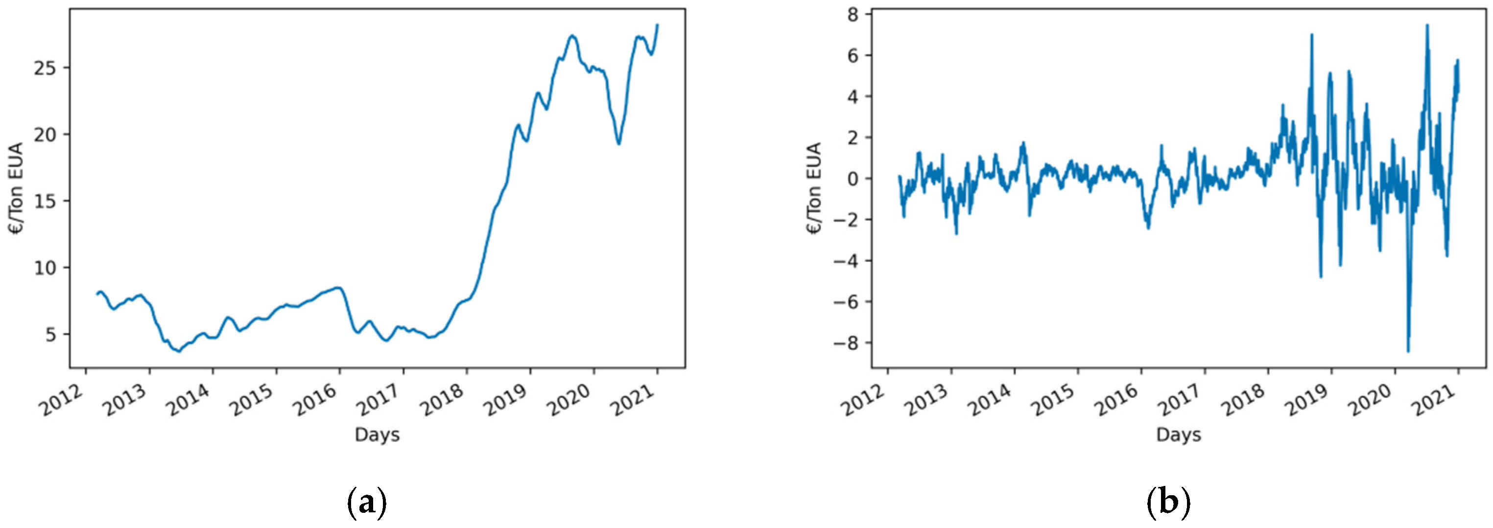
The time series used in this work is the daily spot price of a ton of CO₂ quoted on the European Energy Exchange (EEX) in Leipzig, Germany. It ranges from 14 October 2009 to 1 January 2021 with a total of 2890 data, as seen in Figure 1. This plot shows two different behaviors of prices: a more or less soft evolution with medium and low values until 2018, and a clear rising trend with high values and steep variations after this year. They have been arranged into a time series to train and then validate the performance of the forecasting tools proposed in this work. Only past data of prices have been used to forecast future values.

It is usual in time series forecasting to use the first data (60–80% of them) to train the model and the remaining (40–20%) to validate its performance. Two of such possible divisions have been tested in this work: 60–40% (training-validation) and 80–20%. Training data will be used to learn the times series behavior by adjusting the model’s inner parameters. Once the forecasting tool (neural networks or XGBoost) is trained, the model so obtained is used to forecast with data from the validation dataset (the predictions obtained in this manner will be compared with the actual values of this dataset to obtain a measurement of the forecasting model accuracy).

Conversely, it should be taken into account that validation data with values significantly higher than those used for training and with steep variations (as those at the end of the time series) could jeopardize the accuracy of the forecasting models, as they have a behavior different from those used form training. To find out whether or not this behavior of the data worsens the performance of the forecasting models they will be also tested with a simpler dataset with a less steep evolution: the time series made up with data from 2009 to 2016, where validation data are similar to those used for training. In other words, the last data of the time series, those with higher values and steep variations, have been removed. The different forecasting structures defined in this work will be tested with both datasets and their corresponding performances compared.

The different behavior of both datasets may be better understood when statistical information describing their data distribution is provided. They may be seen in

Table 1. Statistics of the original dataset.

	Original	MinMax	Standard
Data	2890	2890	2890
Mean	11.895	0.297	0.000
Std	7.44	0.224	1.000
Min	2.750	0.000	−1.229
25%	5.920	0.103	−0.803
50%	8.145	0.175	−0.504
75%	15.875	0.427	0.534
Max	33.440	1.000	2.896

and

Table 2. Statistics of the reduced dataset.

	Original	MinMax	Standard
Data	1834	1834	1834
Mean	8.543	0.414	0.000
Std	3.848	0.271	1.000
Min	2.680	0.000	−1.523
25%	5.602	0.206	−0.764
50%	7.185	0.318	−0.352
75%	12.415	0.687	1.006
Max	16.840	1.000	2.156

. The total number of data along their mean values, standard deviation, minimum and maximum values and the values defining each quartile are presented. From these data it may be concluded that the time series from 2009 to 2016 presents a more bonded behavior with lower fluctuations. Information regarding the scaled versions of both datasets (see below) is also provided.

The performance of predictions will be measured with two figures of merit: the Mean Absolute Percentage Error (MAPE) and the Root Mean Squared Error (RMSE):

$$MAPE=\frac{1}{N} {\displaystyle \sum }_{i=1}^N\left|\frac{A_i-F_i }{A_i}\right|·100,$$

(19)

$$RMSE= \sqrt{\frac{1}{N}{\displaystyle \sum }_{i=1}^N{\left(A_i-F_i\right)}^2}$$

(20)

where A_i is an actual datum, F_i a forecasted one and N the total number of data predicted.

3.1. Data Scaling

The structure of the data shown in Figure 1 suggests that it may be difficult for the forecasting tool to provide accurate predictions because a lot of extreme values appear. To overcome this problem, very common in both regression and classification problems, data were scaled before using them, that is to say, they were transformed into a new bounded dataset. In the programming environment used in this work, Python, there are two algorithms which are mainly used to carry out this task: normalization and standardization. The first one transforms the original dataset into another in which values are included in interval [1]. There are several ways to do this, although in this work, the Min-Max one has been selected because of its simplicity:

$$x_i^n=\frac{x_i-x_{min}}{x_{max}-x_{min}}$$

(21)

where $x_i^n$ represents the normalized datum, $x_i$ the original one and $x_{max}$ and $x_{min}$ the maximum and minimum data in the original data set.

The second algorithm transforms the dataset into another one with zero mean and variations normalized to the standard deviation of data. This process is carried out with:

$$x_i^s=\frac{x_i-\overline{x}}{\sigma }$$

(22)

where $x_i^s$ is the standardized datum, $x_i^s$ the mean of the whole data set and $\sigma$ their standard deviation.

Both algorithms will be used with all the forecasting tools used in this work to find out which one provides the best performance. It is worth noting that a process opposite to that of scaling must be applied to the forecasted data. The corresponding expressions will be obtained by reversing Equations (21) and (22).

3.2. Model Simulation

In this work, three artificial intelligence forecasting models have been tested: two Neural Networks (MLP and LSTM) and a popular machine learning tool widely used to solve data science problems, XGBoost. Each model will be simulated with three different preprocessing scenarios: no preprocessing, trend-fluctuations, decomposition, and EMD.

The first preprocessing method consists of splitting the CO₂ emission allowance price series into two subseries (Figure 2): its trend and fluctuations around it. They both will be independently forecasted, and their predictions added to obtain the predicted price.

In the second preprocessing model, the times series is split into eight stationary subseries (Figure 3), IMFs, which are independently forecasted and then added.

Before preprocessing the dataset, it has been scaled with both Min-Max normalization and standardization. The whole sequence of the different actions carried out to perform forecasting is described in the flowchart presented in Figure 4. As it may be seen, the process starts by scaling data and then splitting them into trend-fluctuations or IMF subseries, which are independently forecasted by each model. The predictions obtained are added to obtain the price predictions after rescaling the values provided by those summations. When data are not split, they are directly processed after scaled. This process is the same for both training and validation.

As pointed out above two datasets have been used: a simpler one, in which the data to be forecasted (validation subset) have a more or less stationary behavior, and the whole dataset, in which the data to be forecasted have values higher than those used for training with steep oscillations. The first defines a “simpler” problem without too extreme values and a “smooth” evolution. The second represents a harder problem with data with a different behavior from those used for training. The aim of defining two different scenarios is to check whether or not the forecasting models are able to provide good performances with both “easier” and “more difficult” problems of the same nature.

Regarding the two neural models, different numbers of layers and neurons in each one were tested. Nevertheless, structures with several hidden layers did not provide better performances than those with one only hidden layer. In fact, this last structure outperformed those with several ones. This is a hardly surprising fact for a MLP because, as pointed out above, an MLP with one hidden layer with enough neurons behaves as a universal approximator. The case of LSTM is different, as it is usually used with a high number of layers and neurons, making up what is known as a “deep learning” neural network. However, this structure is applied to very complex problems, such as text or speech processing. Forecasting time series, no matter how nonlinear it is, is a much simpler problem to deal with. Thus, it looks reasonable to accept that a LSTM with one only layer will be enough to obtain accurate predictions. Therefore, only the results obtained with one hidden layer are presented in this work. The best performance was obtained with 100 neurons in the hidden layer for MLP and 100 memory blocks with one only cell in each one for LSTM. In this last network, the depth of the time delays in feedback was 3. Higher values were also tested, but the effect of gradient explosion appeared.

As these neural networks (and XGBoost) carry out a process of time series forecasting, past data of prices are used to forecast future ones. Those past values (several data preceding those to be forecasted) are the inputs to the neural networks (and XGBoost). The number of past data which provides the most accurate predictions should be determined by trial and error; therefore, several numbers of inputs between 1 and 100 were tested with the three models for the two datasets used. For MLP, the best performances were obtained with 60 inputs for the reduced dataset and 3 for the whole one. For LSTM, the best results were obtained with 3 inputs for the 2 datasets.

Several structures were also tested for the XGBoost algorithm. The best results were obtained with 1000 trees with a tree depth of 3 and 3 inputs for the two datasets.

The three forecasting models predicted 20 data at once, that is to say, they provided forecasted values of the daily spot price of CO₂ for the next 20 working days. So, the output layer of both MLP and LSTM has 20 neurons. This value was selected because it represents predictions for almost one month, four weeks, as the European Energy Exchange does not work at weekend days. The aim of providing 20 future values is to obtain both short-term and long-term predictions at once with one only forecasting model. The accuracy of the predictions (errors) will refer to that of 1 day ahead, 2 days ahead, and so on for the 20 predicted data.

All simulations have been programmed in Python with Tensor Flow and Keras packages. The XGBoost library for Python has been also used. The programs have been run in a personal computer with an Intel core i7-9700, 3.6 GHz with 32 Gbytes of RAM memory. Simulations have intensively used the GPU included in a RTX 2070 SUPER graphic card from Nvidia.

3.3. Prediction with MLP

The prediction errors (RMSE and MAPE) obtained with MLP are presented for both the simplified dataset and the whole one in

Table 3. Predictions with MLP for the reduced data set (2009–2016). 60% of them were used for training and 40% for validation. Data have been scaled with standardization for “Without Prep.” and “Trend-Fluc.” and with Min-Max for EMD.

Days Ahead	Without Prep.		Trend-Fluc.		EMD (3 Inputs)		EMD (60 Inputs)
	RMSE	MAPE	RMSE	MAPE	RMSE	MAPE	RMSE	MAPE
1	0.19	2.38	0.21	2.59	0.13	1.59	0.20	2.47
2	0.23	2.94	0.25	3.05	0.15	1.84	0.21	2.69
3	0.26	3.27	0.27	3.48	0.15	1.81	0.21	2.66
4	0.29	3.60	0.32	4.01	0.25	3.38	0.22	2.83
5	0.32	4.22	0.36	4.53	0.18	2.21	0.24	3.00
6	0.35	4.52	0.38	4.79	0.20	2.53	0.24	2.95
7	0.39	4.97	0.40	5.13	0.21	2.73	0.22	2.73
8	0.41	5.25	0.43	5.41	0.24	3.12	0.24	3.04
9	0.42	5.35	0.49	6.11	0.25	3.23	0.26	3.32
10	0.45	5.77	0.52	6.43	0.26	3.41	0.27	3.42
11	0.48	6.04	0.55	6.76	0.26	3.41	0.26	3.29
12	0.51	6.41	0.57	7.00	0.28	3.68	0.27	3.42
13	0.53	6.66	0.63	7.81	0.31	4.04	0.33	4.31
14	0.53	6.67	0.63	7.72	0.36	4.80	0.30	3.74
15	0.55	6.90	0.67	8.23	0.32	4.18	0.35	4.54
16	0.58	7.23	0.67	8.22	0.34	4.53	0.29	3.64
17	0.59	7.42	0.71	8.71	0.38	5.04	0.32	3.90
18	0.62	7.74	0.75	9.15	0.36	4.71	0.31	3.91
19	0.64	7.92	0.75	9.19	0.40	5.33	0.34	4.49
20	0.64	7.99	0.77	9.42	0.40	5.24	0.35	4.44
Mean	0.45	5.66	0.52	6.39	0.27	3.54	0.27	3.44
Std	0.14	1.69	0.18	2.11	0.08	1.15	0.05	0.64

and

Table 4. Predictions with MLP for the whole data set (2009–2020). 80% of them were used for training and 20% for validation. Data have been scaled with standardization for “Without Prep.” and “Trend-Fluc.” and with Min-Max for EMD.

Days Ahead	Without Prep.		Trend-Fluc.		EMD
	RMSE	MAPE	RMSE	MAPE	RMSE	MAPE
1	0.72	2.19	0.72	2.24	0.92	2.91
2	0.97	2.99	0.96	2.99	0.97	3.14
3	1.18	3.66	1.16	3.66	1.01	3.26
4	1.35	4.18	1.31	4.13	1.08	3.48
5	1.51	4.60	1.49	4.67	1.16	3.68
6	1.64	5.05	1.63	5.11	1.19	3.75
7	1.74	5.42	1.75	5.47	1.22	3.91
8	1.86	5.77	1.82	5.76	1.28	4.05
9	1.94	6.19	1.91	6.01	1.35	4.30
10	2.04	6.47	2.00	6.23	1.45	4.69
11	2.13	6.72	2.08	6.43	1.42	4.52
12	2.20	6.98	2.15	6.71	1.48	4.78
13	2.28	7.25	2.23	6.91	1.52	4.85
14	2.38	7.52	2.31	7.15	1.55	4.98
15	2.45	7.73	2.39	7.41	1.60	5.03
16	2.53	7.89	2.46	7.64	1.64	5.22
17	2.64	8.29	2.53	7.86	1.69	5.43
18	2.70	8.49	2.62	8.15	1.73	5.51
19	2.78	8.64	2.65	8.35	1.76	5.68
20	2.86	9.00	2.74	8.68	1.77	5.65
Mean	2.00	6.25	1.95	6.08	1.39	4.44
Std	0.60	1.92	0.57	1.78	0.27	0.85

. Several divisions of data for training and validation were tested and the best results were obtained with 60–40% for the first dataset and 80–20% for the second. This is hardly surprising, because the first one takes into account data with values similar to those to be forecasted in the training subset, nevertheless for the whole dataset a division of 60–40% does not consider data with a steep rising trend for training, while in that of 80–20% a lot of data with that behavior are used.

The results in Table 3 show that the best performance was obtained when EMD was used to preprocess the reduced dataset. Nevertheless, although the best results were obtained with 60 inputs, a noticeable result was also obtained with a lower number of inputs (3): while the short-term horizon predictions are clearly improved those of the long-term ones got worse, providing a wider range of errors (as the higher standard deviation obtained shows). So, they both have been included in Table 3 as structures providing the best performance. It is difficult to decide which of them is the most accurate; in fact, it becomes a matter of preference; it depends on which prediction horizon the user is interested in.

The results obtained when the whole dataset was used (Table 4) show that, again, the best predictions were obtained when EMD was used to preprocess the input data. It is worth noting that these results were obtained, in all cases, with only 3 inputs.

When comparing the results obtained with the two datasets, it may be seen that those obtained with the whole dataset are worse than those obtained with the reduced one. Nevertheless, these worse results are not too high, and it may be stated that reliable predictions were obtained. This fact shows the robustness of MLP as a forecasting tool, as its performance has suffered only a slight worsening when dealing with more complex data. In addition, it only needed three inputs to provide those results with the whole dataset, a structure much simpler than that with 60 inputs for the reduced one.

3.4. Prediction with LSTM

Table 5. Predictions with LSTM for the reduced data set (2009–2016); 60% of them were used for training and 40% for validation. Data have been scaled with standardization for “Without Prep.” and “Trend-Fluc.” and with Min-Max for EMD.

Days Ahead	Without Prep.		Trend-Fluc.		EMD
	RMSE	MAPE	RMSE	MAPE	RMSE	MAPE
1	0.18	2.14	0.16	1.91	0.48	5.61
2	0.23	2.77	0.22	2.72	0.48	5.64
3	0.26	3.29	0.27	3.32	0.50	5.95
4	0.30	3.74	0.31	3.88	0.50	5.90
5	0.33	4.18	0.35	4.39	0.48	5.81
6	0.36	4.57	0.39	4.92	0.51	6.13
7	0.39	4.90	0.43	5.41	0.52	6.39
8	0.41	5.27	0.46	5.89	0.50	6.16
9	0.44	5.59	0.50	6.34	0.49	6.14
10	0.46	5.88	0.53	6.75	0.52	6.42
11	0.49	6.14	0.56	7.14	0.60	7.51
12	0.51	6.40	0.59	7.54	0.51	6.42
13	0.53	6.66	0.62	7.91	0.61	7.69
14	0.56	6.91	0.65	8.32	0.55	6.98
15	0.58	7.17	0.68	8.71	0.56	7.08
16	0.60	7.42	0.70	9.08	0.62	7.81
17	0.62	7.66	0.73	9.46	0.57	7.30
18	0.63	7.89	0.75	9.80	0.61	7.75
19	0.65	8.10	0.78	10.12	0.59	7.51
20	0.67	8.32	0.80	10.36	0.68	8.82
Mean	0.46	5.75	0.52	6.70	0.54	6.75
Std	0.14	1.80	0.19	2.51	0.06	0.87

and

Table 6. Predictions with LSTM for the whole data set (2009–2020). 80% of them were used for training and 20% for validation. Data have been scaled with standardization for “Without Prep.” and “Trend-Fluc.” and with Min-Max for EMD.

Days Ahead	Without Prep.		Trend-Fluc.		EMD
	RMSE	MAPE	RMSE	MAPE	RMSE	MAPE
1	0.95	2.94	0.76	2.43	4.36	17.32
2	1.13	3.57	0.98	3.16	4.40	17.38
3	1.30	4.11	1.17	3.76	4.39	17.28
4	1.45	4.56	1.32	4.24	4.41	17.30
5	1.60	5.01	1.49	4.75	4.32	16.83
6	1.72	5.42	1.62	5.15	4.49	17.47
7	1.82	5.80	1.72	5.48	4.41	17.04
8	1.91	6.12	1.80	5.74	4.42	17.00
9	2.00	6.47	1.88	5.90	4.41	16.84
10	2.09	6.83	1.95	6.08	4.38	16.63
11	2.18	7.13	2.03	6.28	4.47	16.89
12	2.25	7.33	2.11	6.53	4.54	17.11
13	2.34	7.65	2.18	6.77	4.41	16.49
14	2.44	7.96	2.27	7.01	4.47	16.63
15	2.51	8.18	2.35	7.26	4.48	16.59
16	2.57	8.29	2.43	7.50	4.19	15.22
17	2.65	8.50	2.51	7.76	4.21	15.16
18	2.72	8.73	2.59	8.04	4.39	15.78
19	2.78	8.97	2.64	8.28	4.30	15.30
20	2.85	9.18	2.71	8.51	4.47	15.87
Mean	2.06	6.64	1.93	6.03	4.40	16.61
Std	0.55	1.83	0.55	1.68	0.09	0.73

show the results obtained with the two datasets used. The best results were obtained with a distribution training-validation 60–40% for the reduced data set and 80–20% for the whole one, a distribution equal to that obtained with MLP. Results in Table 5 shows that now the best performance was obtained when no preprocessing was applied to the reduced dataset. The accuracy obtained when data were preprocessed by splitting them into trend and fluctuation was slightly better for the first two forecasted data than those without preprocessing, although they are clearly worse for the remaining ones. Data preprocessed with EMD provide clearly worse predictions than the option without preprocessing for short-term forecasting, although similar results were obtained for the long-term ones. When compared with the trend-fluctuations decomposition, it provides significantly worse results for short-term predictions, while providing better results for long-term ones.

Performances when the whole dataset was used are shown in Table 6. Now the best accuracy was obtained with the trend-fluctuations preprocessing, although it was only slightly better than that obtained without preprocessing. It provides an accuracy only slightly worse than that obtained without preprocessing when the reduced dataset was used (the best option for that case), and clearly better for the last forecasted data when the same preprocessing process was applied to the reduced dataset. Nevertheless, the results obtained when the data were preprocessed with EMD are surprisingly poor, and what is more, long-term predictions are slightly better than short-term ones. They are much worse than those obtained with the reduced dataset. So, it may be stated that LSTM when EMD preprocessing was used has not been able to deal with the steep changes that appear at the end of the whole time series, while the structures without preprocessing and with trend-fluctuations decomposition were able to provide predictions that are only slightly worse that those obtained with the reduced dataset. This fact shows the robustness of LSTM with those two preprocessing models, as their performance suffers only a slightly worsen when a more complex time series is forecasted.

3.5. Prediction with XGBoost

The results obtained with XGBoost are shown in

Table 7. Predictions with XGBoost for the reduced data set (2009–2016). 60% of them were used for training and 40% for validation. Data have been scaled with standardization for “Without Prep.” and “Trend-Fluc.” and with Min-Max for EMD.

Days Ahead	Without Prep.		Trend-Fluc.		EMD
	RMSE	MAPE	RMSE	MAPE	RMSE	MAPE
1	0.18	2.26	2.06	2.58	0.59	7.91
2	0.25	3.21	2.77	3.56	0.61	8.09
3	0.30	3.81	3.32	4.32	0.62	8.19
4	0.36	4.60	3.77	4.92	0.63	8.27
5	0.41	5.21	4.30	5.65	0.64	8.32
6	0.46	5.98	4.79	6.30	0.65	8.30
7	0.52	6.75	5.25	6.95	0.65	8.31
8	0.58	7.49	5.76	7.65	0.66	8.36
9	0.62	7.99	6.16	8.23	0.65	8.34
10	0.68	8.82	6.68	8.94	0.66	8.26
11	0.74	9.52	7.29	9.75	0.66	8.33
12	0.78	10.15	7.76	10.37	0.66	8.22
13	0.82	10.66	8.19	10.99	0.66	8.23
14	0.84	10.96	8.54	11.53	0.66	8.12
15	0.88	11.41	8.98	12.14	0.66	8.19
16	0.91	11.82	9.38	12.65	0.66	8.27
17	0.94	12.21	9.82	13.27	0.66	8.26
18	0.96	12.50	10.07	13.61	0.66	8.30
19	0.97	12.57	10.32	13.92	0.67	8.43
20	0.99	12.78	10.57	14.28	0.68	8.62
Mean	0.66	8.54	6.79	9.08	0.65	8.27
Std	0.26	3.35	2.63	3.62	0.02	0.14

and

Table 8. Predictions with XGBoost for the whole data set (2009–2020). 80% of them were used for training and 20% for validation. Data have been scaled with standardization for “Without Prep.” and “Trend-Fluc.” and with Min-Max for EMD.

Days Ahead	Without Prep.		Trend-Fluc.		EMD
	RMSE	MAPE	RMSE	MAPE	RMSE	MAPE
1	3.40	9.72	2.60	8.66	30.49	123.22
2	3.39	10.14	2.75	9.29	30.48	123.14
3	3.73	11.50	2.84	9.67	30.52	123.20
4	3.40	10.78	2.93	10.07	30.50	123.05
5	3.55	11.51	3.06	10.47	30.41	122.65
6	3.66	11.98	3.06	10.56	30.40	122.50
7	3.44	11.37	3.14	10.83	30.39	122.35
8	3.63	12.06	3.19	11.04	30.39	122.30
9	3.68	12.38	3.23	11.13	30.39	122.19
10	2.93	9.61	3.29	11.33	30.37	121.96
11	2.88	9.33	3.36	11.61	30.36	121.84
12	2.84	9.07	3.39	11.69	30.31	121.49
13	3.00	9.60	3.49	12.02	30.34	121.53
14	3.28	10.63	3.63	12.58	30.33	121.44
15	3.32	10.64	3.73	12.85	30.34	121.39
16	3.62	11.71	3.78	12.91	30.31	121.10
17	3.69	11.87	3.85	13.04	30.30	120.95
18	3.97	12.89	3.93	13.23	30.31	120.90
19	3.95	12.77	4.03	13.48	30.27	120.66
20	4.25	14.00	4.08	13.74	30.30	120.70
Mean	3.48	11.18	3.37	11.51	30.38	121.93
Std	0.37	1.31	0.43	1.43	0.07	0.84

. The first one presents the results obtained with the reduced dataset with a 60–40% division for training and validation and the second those with the whole one and an 80–20% division. The best performance obtained with the reduced dataset (Table 7) may be assumed as that provided by the model without preprocessing. Nevertheless, this statement demands a detailed explanation. The mean error of the twenty predictions is 8.54% for this model although that obtained with the EMD decomposition is 8.27%. However, the errors provided by this last model are almost constant for all predictions (as their very low standard deviation shows), while those obtained with the model without preprocessing are lower for the short-term predictions and higher for the long-term ones (higher standard deviation). This represents a more logical behavior of the forecasting tool, which provides a balanced evolution, since predictions get worse as the time horizon increases. But if the user considers-long-term predictions as more valuable than short-term ones, the best model should be that with EMD decomposition.

The predictions obtained with the whole dataset (Table 8) are clearly worse that those obtained with the reduced one. The best performances were obtained with both the trend-fluctuation decomposition and without it, and it is surprising that the performance obtained with the EMD decomposition is especially bad. The errors are almost constant but with a so high value that it must be discarded as a forecasting model. When comparing the results obtained by the two datasets (only for no preprocessing and the trend-fluctuation decomposition) it may be seen that predictions get worse for the short-term remaining similar for the long-term. This means that XGBoost have problems to deal with a more complex dataset, at least in the short-term.

4. Discussion

When comparing the performance of the models simulated, it is clear that both MLP and LSTM outperform XGBoost in all cases. Only short-term predictions errors when no preprocessing and trend-fluctuations were used with the reduced dataset were similar to those of MLP or LSTM. For the whole dataset, errors are so high, especially in the case of EMD, that it may be stated that XGBoost is not a useful tool for forecasting this time series. This is not surprising if one bears in mind that XGBoots was designed to carry out classification tasks, so that it is not well suited for time series prediction. As it is proved in this work, XGBoost is not able to provide better results than other machine learning tools usually used in time series forecasting, such as the neural models used here.

Both MLP and LSTM were able to provide good predictions with the simplified dataset. In fact, very similar results were obtained when forecasting without preprocessing and when the trend-fluctuations were used: mean errors of 5.66% for MLP and 5.75% for LSTM without preprocessing and 6.39 and 6.70% for the trend-fluctuation preprocessing were obtained. This data also show that the accuracy of both models gets worse for the trend-fluctuations decomposition. Nevertheless, the performance of MLP is clearly improved when EMD is applied to the dataset (mean errors of 3.44 and 3.54%) while that of LSTM remains unchanged (mean error of 6.75%). As pointed out before, two structures have been tested with the MLP-EMD model because, although they provided almost equal mean errors, the time evolution of the prediction accuracies clearly differ: the structure with 3 inputs provides lower errors for short-term predictions, while that with 60 ones is better for long-term. From these results, it may be stated that the performance of MLP is clearly improved when EMD is applied, so that this structure provides the best performance of all the models tested with this dataset.

When the whole dataset is used, both MLP and LSTM provide similar results when no preprocessing was used (mean error of 6.25% for MLP and 6.64% for LSTM) and with the trend-fluctuations preprocessing (6.08 and 6.03%, respectively). However, their behavior clearly differs when preprocessed with EMD: while the mean error provided by MLP clearly decreases, providing a mean error of 4.44%, that obtained with LSTM undergoes a strong increase to 16.61%.

When comparing the results provided by MLP and LSTM with the two datasets, it may be seen that they are very similar, with a slight increase when no preprocessing was used (they pass from 5.66 and 5.75% for MLP and LSTM, respectively, with the reduced dataset to 6.25 and 6.64% with the whole one) and a slight decrease when trend-fluctuation was applied (6.39 and 6.70% to 6.08 and 6.03%).

These facts prove the robustness of MLP and LSTM when forecasting time series, as they are able to provide accurate prediction with both simpler and more complex time series providing that the training dataset is properly selected (the whole dataset was split into an 80–20% decomposition for the training-validation division instead of the 60–40% used for the reduced one).

Both MLP and LSTM are able to provide equally accurate predictions when they carry out forecasting directly, without preprocessing, achieving very similar errors. This common behavior changes when preprocessing is included. They both provide similar mean results when trend-fluctuations are included, although MLP behaves better for long-term predictions while LSTM does for short-term ones; but, for the reduced dataset, when EMD is included, MLP is able to improve its performance by decreasing its mean error to 3.44 and 3.54%, whereas LSTM is only able to provide a mean error almost equal to that obtained with trend-fluctuations (although now with worse errors for short-time predictions). This behavior is more striking for the whole data set, since while MLP clearly improves accuracy when EMD was applied (its mean error falls to 4.44%) LSTM undergoes a strong increase to 16.16% and, what is more striking, with all values very close to that mean.

Therefore, it may be stated that both MLP and LSTM are able to provide accurate and robust prediction when no preprocessing is included in the forecasting model, but when it is included MLP clearly improves its performance when EMD is used, whereas LSTM provides much worse results, in fact the worst ones achieved with the three options tested.

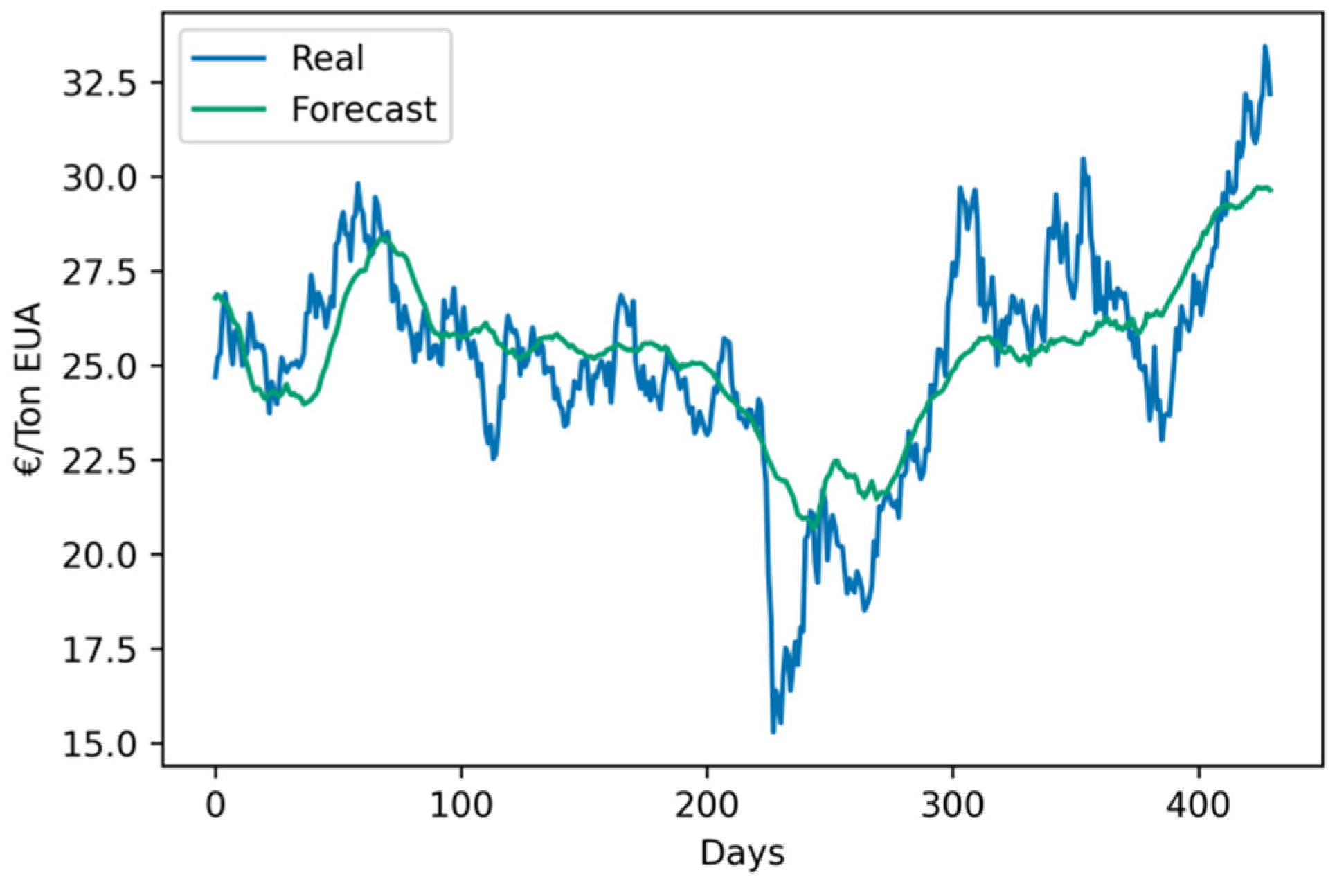
On the other hand, it may be very interesting to analyze the evolution of predictions regarding their time horizon in order to identify how they behave, and their accuracies evolve. To do that, the one-day-ahead and the twenty-days-ahead predictions obtained in the validation set of the whole dataset provided by MLP-EMD are presented in Figure 5 and Figure 6. It may be seen in Figure 5 that one-day-ahead predictions are able to follow fluctuations of CO₂ price, providing a reliable estimation of its daily evolution. Nevertheless, predictions with a time horizon of 20 days, as seen in Figure 6, are not able to follow daily fluctuations but, instead, they represent a sort of mean value of fluctuating prices, in other words, they provide a sort of trend of the time evolution of CO₂ prices. So, it could be stated that the model provides a prediction of the trend of the price evolution for the long-term instead of an estimation of actual prices on that time horizon. This behavior may be very useful for traders interested in the long-term evolution of prices because those predictions describe a sort of trend of how they will evolve.

This twofold behavior of the predicted data may be very useful, because it provides valuable information to agents involved in purchasing and selling EUAs. They can serve as a reference for managers of companies included in the EU ETS, as they can manage their allowances portfolio with reliable information to help them make decisions about their costs in the short-term. In addition, long-term forecasts may be very useful for managers of polluting companies, as they provide fairly tight predictions of the price evolution trend. The proposed model gives reliable trend information, with a time horizon that is more suitable for making decisions on decarbonization in production processes.

5. Conclusions

Forecasting daily spot prices of CO₂ has become a key issue in recent years due to its upward trend that is affecting the final price of electricity. Several tools may be used to carry out this task, although Neural Networks seem to be the most reliable option, since they have proved to be one of the most accurate tools for time series forecasting. Nevertheless, not all models are able to provide accurate and reliable predictions and the best option for each particular time series should be identified by testing several ones. In this work, two popular neural models (MLP and LSTM) have been used to forecast the time series of daily spot prices of CO₂. Another popular artificial intelligence tool (XGBoost) has been also used for the sake of comparison. It provided poor performance compared with those obtained with the neural models. Several works have proved that the prediction accuracy of the forecasting models may be significantly improved when a suitable data preprocessing is applied prior to carry out the forecasting process. Thus, in this work, two techniques have been tested, trend-fluctuation decomposition and EMD, to provide data preprocessing. The best results were obtained with a hybrid MLP-EMD model, which provided a significant decrease in the forecasting errors. However, several of the combinations tested were not able to overcome the corresponding single forecasting tool, providing, in some cases, significantly higher errors. The robustness of the proposed models has been tested by using two datasets: a simplified one with a soft evolution and an enlarged one that included updated data with a rising trend with steep variations. The combination of MLP-EMD was able to provide accurate and reliable predictions with them both. Only a small increase of forecasting errors with the enlarged dataset was obtained, a fact that proves the model to be a robust forecasting tool. It is worth noting that MLP clearly outperforms LSTM as a forecasting tool despite the fact that this last seems, at first glance, to be better fitted for time series forecasting because of its recurrent behavior and inner “memory”. In fact, MLP has proved to be a more accurate and robust forecasting tool. In addition, it has been able to take advantage of preprocessing techniques to improve accuracy while LSTM was not.

Therefore, an accurate and robust forecasting tool has been proposed to predict the time evolution of the daily spot price of CO₂. Predictions for 20 working days (four weeks) are provided at once with good accuracy, as means error of 2.91 % for the nearest prediction (1 day ahead) and 5.65% for the furthest one (20 days ahead) were provided. Thus, it may be a very useful tool for enterprises selling and purchasing emission allowances as well as for electric energy trading companies, as the forecasting model presented in this work is able to provide reliable predictions of the time evolution of daily spot prices of CO₂, what may help them to make decisions concerning their selling or purchasing activities.

On other hand, obtaining reliable allowance price predictions is important to market participants (such as affected companies, traders or brokers) who need accuracy price predictions to better manage their portfolios. Moreover, it is also crucial for the design of environmental policies, since CO₂ emission allowance prices provide information on the marginal abatement costs in the industry. Thus, based on the evolution of prices, the effectiveness of the environmental policies can be evaluated and the emission cap adjusted. Therefore, a more accurate carbon price forecasting is essential to establish a stronger and more efficient emission market.

Based on the results presented in this work, we aim at carrying out further research to test the efficiency of preprocessing strategies different from those used here. Refinements of EMD such as Ensemble Empirical Mode Decomposition (EEMD) or Variational Mode Decomposition (VMD) could be applied and their performances compared with those obtained in this work. In addition, a study of different strategies to split data into training and validation sets based on cross-validation should also be carried out to try to define a model independent of the training-validation division dependence of accuracy pointed out in this work.