A Method to Improve the Accuracy of Simulation Models: A Case Study on Photovoltaic System Modelling

Abstract

This research presents a method to improve data accuracy for the more efficient data management of the studied applications. The data accuracy was improved using the preciseness function learning model (PFL model). It contains a database in which the amount of data is more or less dependent on all of the possible behavior of the studied application. The proposed model improves data with functions obtained by optimizing curves to represent the data at each point, which estimate the database’s diffusion behavior, and functions can be built around all of the various forms of databases. The proposed model always updates its database after processing. It has been learning to optimize the processing precision. In order to verify the precision of the proposed model through its application to a PV system simulation model, the process’s database should contain at least one year. This is because the overall behavior of the PV power output in Thailand depends on the seasonal weather; Thailand has three seasons in a period of one year. The testing was performed by comparing the PV power output. The simulation results with the actual measurement data (12 MW PV system) can be divided into two conditions: the daily comparison and the seasonal PV power output. As a result, the proposed model can accurately simulate the PV power output despite the sudden daily climate change. The average nRMSE (normalized RMSE) of the proposed model is very low (1.23%), and ranges from 0.30% to 2.26%. Therefore, it has been proven that this model is very accurate.

1. Introduction

The application of mathematical models makes process improvement more convenient because sometimes it is not able to perform experiments and modify the processes. The model helps us to obtain in-depth information to be used for the benefits of education or business. The adequacy of the model which is used relies on its accuracy in processing the results. Suppose the model has low accuracy; it will cause more disadvantages than benefits. The primary source of this research will be a recognition of the importance of the model’s accuracy. At present, photovoltaic generators have been installed as a substitute for various sources of electrical energy, for applications such as home appliances, utilities, external battery packs, and generators, etc. The most critical steps after the installation of the PV system are maintenance and checking. If we estimate the PV system’s energy production, we will be available to check for system faults by comparing the measured data with the simulation data for energy management, and checking whether it exceeds its maximum benefit. Data accuracy is a critical factor for effective energy data management. As such, this research will present a PV system estimation model with a preciseness function learning model.

Many researchers have conducted studies on the creation of PV models, from one-panel simulations to systems simulations of solar cells. PV models are mainly affected by the module temperature and solar irradiance. Most of the modeling research is the analysis of single-diode equivalent circuits (five parameters model) [1,2,3,4,5,6,7,8,9,10,11,12,13,14,15,16,17,18]. These models have five parameters: photocurrent, the ideal factor according to the photovoltaic technology, parallel resistance, leakage current, and series resistance. In many studies, the data accuracy has been improved after simulating the data from the model by different methods. For example, the improvement of the accuracy of PV models by the use of weight functions obtained by 1-year measured data has been studied [1]. This method makes the model more accurate by evaluating the database using a polynomial equation. This equation is a data evaluation in one form of a curve-fitting process. Other research has shown the linear weighting method for PV power forecasting models [2]. This method updates the model data using a linear equation in order to obtain the final result. Based on several studies on the improvement of the accuracy of the database, each method [3,4,5,6] has different strengths depending on the distribution behavior of the database. Therefore, this research combines each method’s strengths and develops it as a new data precision improvement method in order to make the model more efficient for the best data management.

This research aims to improve the processing accuracy of models in order to make the models more useful. The method used to improve the data accuracy is the incorporation of the strengths of the creation of a function from a database to solve problems if a high distribution of information is created. This model can be made more effective by adding output data into the database to enable the model to be self-learning, and to calculate more precisely in the next calculations. The case studies applied to this process were the power output simulation model of photovoltaic systems, and comparison of the efficiency with the other methods or processes of accuracy improvement researched earlier. The test used data from photovoltaic systems in Thailand (14°10′78.1″ north latitude and 100°16′94.9″ east longitude). There were two inputs in this model, which are solar irradiance and module temperature, and the output of the model was the power output value of the photovoltaic system. The test was to bring the PV power output value from the accuracy improved model in the different forms, including this research process compared to the actual PV power output in three seasons: the summer, the rainy season, and the winter. The climate changes of the target area have a profound effect on the performance of photovoltaic systems, and also the timing of the installation of the system that causes energy loss in various fields. For this reason, the research devised a method to optimize the data accuracy of the PV system simulation model in order to be as accurate as possible in any climate change. The proposed model detects an abnormality in the power generation of the system and uses the obtained data to check the system for the most efficient system.

2. Materials and Methods of the PV System Simulation Model

2.1. Proposed Model for Accuracy Improvement (Interactive Curve Fitting)

The model was created from the analysis of the most suitable curve to represent the data in each point of interest in order to estimate the value of the data, which is called a ‘curve-fitting process’ [19,20], and to select the target function in many forms for analysis, which is called the ‘optimization process’. The functions used in this model are shown as follows.

Exponential models provide a 1-term and a 2-term exponential model given by Equations (1) and (2).

$${\psi }_{exp,1}=a{e}^{bx}$$

(1)

$${\psi }_{exp,2}=a{e}^{bx}+c{e}^{dx}$$

(2)

Exponential models are often used when the quantity’s rate of change is proportional to the quantity’s initial amount. If the coefficient associated with b and/or d is negative, y represents exponential decay. If the coefficient is positive, y represents exponential growth.

The Fourier series models are the summation of the sine and cosine functions that describe a periodic signal. It represents them in either the trigonometric form or the exponential form. This fitting curve, shown in Equation (3), provides this trigonometric Fourier series form:

$${\psi }_{ft}=a_o+{{\displaystyle \sum }}_{i=1}^{n_f}{a}_{i}cos\left(iwx\right)+b_{i}sin\left(iwx\right)$$

(3)

where a_o is the model’s a constant (intercept) term in the data, and is associated with the i = 0 cosine term; w is the signal’s fundamental frequency; n_f is the number of terms (harmonics) in the series 1 ≤ n_f ≤ 5.

The Gaussian model fits peaks; and is given by

$${\psi }_{gs}={{\displaystyle \sum }}_{i=1}^{n_g}{a}_i{e}^{\left[-{\left(\frac{x-b_i}{c_i}\right)}^2\right]}$$

(4)

where a is the amplitude, b is the centroid, c is related to the peak width, and n_g is the number of peaks to fit; this provides a 1-term and a 2-term Gaussian model.

Polynomial models for curves are given by

$${\psi }_p={{\displaystyle \sum }}_{i=1}^{n_p+1}{p}_i{x}^{n_p+1-i}$$

(5)

where n_p + 1 is the polynomial order, n_p is the polynomial degree, and 1 ≤ n_p ≤ 5. The order gives the number of coefficients to be fitted, and the degree gives the highest power of the predictor variable.

The sum of sines model fits periodic functions, and is given by

$${\psi }_{si}={{\displaystyle \sum }}_{i=1}^{n_{si}}{a}_{i}sin\left(b_{i}x+c_i\right)$$

(6)

where a is the amplitude, b is the frequency, and c is the phase constant for each sine wave term. n_si is the number of terms in the series, and it provides 1-term and a 2-term Sum of Sines models.

Each of the methods above is estimated to be accurately calculated as a function based on the studied database’s distributed behavior.

2.2. One Diode Equivalent Circuit

In order to understand solar cells’ electrical properties, the equivalent circuit of solar cells [7,8]—as shown in Figure 1—was considered. The solar cell consists of a constant current source, which is the current of the solar cells caused by the solar irradiance (I_ph), the p–n junction of a diode, the series resistance in the solar cell (R_s), and the parallel resistance within the solar cell (R_sh).

The photocurrent (I_ph) from solar irradiance will be divided through the diode and R_s, and then load (R_L). The current flowing through R_s and R_L is I.

$$I_{ph}=I_d+I$$

(7)

$$I=I_{ph}-I_d$$

(8)

where I_ph is photocurrent (A), I_d is the current generated by the diode (A), and I is current that the solar cells produce (A).

When R_s = 0, and I_d is given by

$$I_d=I_0\left[exp\left(\frac{q{V}_0}{nk{T}_m}\right)-1\right]$$

(9)

where I_d is the current generated by the diode (A), I_o is the reverse saturation current of the diode (A), q is the electron charge value (1.602 × 10⁻¹⁹ C), k is the Boltzmann constant (1.381 × 10⁻²³ J/K), T_m is the actual temperature at the PV module (K), R_s is the series resistance (Ω), R_sh is the shunt or parallel resistance (Ω), and n is the ideal factor of a diode according to the PV technology involved (chosen from

Table 1. The ideal factor depends on the PV technology [18,21].

PV Technology	Values
Monocrystalline	1.2
Polycrystalline	1.3
CdTe	1.5
CIS	1.5
GaAs	1.3
Amorphous silicon single junction	1.8
Amorphous silicon double junction	3.3
Amorphous silicon triple junction	5.0

).

By substituting Equation (9) into Equation (8), we obtain Equation (10):

$$I=I_{ph}-I_0\left[exp\left(\frac{q{V}_0}{nk{T}_m}\right)-1\right]$$

(10)

In the case of a short-circuit, the load to obtain the maximum current value of the solar cell (I_sc), V_o = 0, is given by

$$I=I_{ph}=I_{sc}$$

(11)

In this case, the photocurrent (I_ph) is I_sc, and is equal to the current generated by the solar irradiance. The circuit is opened at the load point for the maximum solar cell voltage (V_oc), I = 0, and V_o = V_oc.

$$I_{ph}=I_0\left[exp\left(\frac{q{V}_{oc}}{nk{T}_m}\right)-1\right]$$

(12)

$$ln\frac{I_{ph}}{I_0}=\frac{q{V}_{oc}}{nk{T}_m}-1$$

(13)

$$\mathrm{S}\mathrm{o}: V_{oc}=\frac{nk{T}_m}{q}\left(ln\frac{I_{ph}}{I_0}+1\right)$$

(14)

where I_ph is the photocurrent (A), I_o is the reverse saturation current of the diode (A), q is the electron charge value (1.602 × 10⁻¹⁹ C), k is the Boltzmann constant (1.381 × 10⁻²³ J/K), T_m is the actual temperature at the PV module (K), V_oc is the open-circuit voltage (V), and n is the ideal factor of a diode according to the PV technology involved (chosen from Table 1).

In the case of the load having 0 < R_L < infinitely, the solar cell supplies current (I) and voltage (V) to the load between 0 < I < I_sc and 0 < V < V_oc. The values of the current and voltage that cause both volumes to have the highest value are called the maximum current and the maximum voltage, respectively. This gives the maximum electric power, as shown in Figure 2.

2.3. Effects of the Series Resistance and Parallel Resistance of Solar Cells

From the equivalent circuit of a solar cell, as shown in Figure 3, while operating, it can be seen that the current from solar irradiance is represented by a constant current source (I_ph). It emits an electrical current in the opposite direction to the current that flows through the p–n junction in ideal (I_d).

The series resistance occurred because of the semiconductor’s resistance, the resistance of the ommic contact area between the metal and the p and n parts, the resistance of the connecting wires, and the sum of all of the series resistance, abbreviated as R_s. Parallel resistance, R_sh, is a hypothetical resistance parallel to the boundary in the complete p–n junction.

Ideally, the value of R_sh is infinite and, in the ideal solar cell, the value of R_s is zero. However, in practice, the semiconductor crystal has a breakdown. Joints, especially those with large areas, have defective parts, resulting in an incomplete p–n junction. Therefore, the R_sh value is not infinite, and the result of the R_s value is not equal to zero. The effects of the R_s and R_sh values will change the properties of the solar cells. In general, the R_sh is not high enough to ignore the effect on the solar cell properties, but the R_s resistance will significantly affect the solar cell properties. In designing the structure’s characteristics, the builders must then consider the effect of the R_s value.

R_s = 0 and I are given by

$$I=I_{ph}-I_0\left[exp\left(\frac{q{V}_0}{nk{T}_m}\right)-1\right]$$

(15)

If R_s > 0 and R_sh < infinity, V₀ = V_L + IR_s is given by

$$I=I_{ph}-I_0\left[exp\left(\frac{q\left(V_L+I{R}_s\right)}{nk{T}_m}\right)-1\right]-\frac{\left(V_L+I{R}_s\right)}{R_{sh}}$$

(16)

where I_ph is the photocurrent (A), I₀ is the reverse saturation current of the diode (A), q is the electron charge value (1.602 × 10⁻¹⁹ C), k is the Boltzmann constant (1.381 × 10⁻²³ J/K), T_m is the actual temperature at the PV module (K), R_s is the series resistance (Ω), R_sh is the shunt or parallel resistance (Ω), and n is the ideal factor of a diode according to the PV technology involved (chosen from Table 1).

From Equation (16) and Figure 4 showing R_s’ effect on solar cells, it can be seen that solar cells with a high R_s value will suffer fewer short-circuit currents. The slope of the graph was also decreased, resulting in much less energy from the solar cells. Therefore, when creating solar cells, there should be a way to reduce R_s to the minimum possible.

2.4. Effect of Solar Irradiance on the Solar Cells

The solar irradiance has a great effect on how the solar cell’s electric current and power change, as shown in Figure 5.

When V = 0, I is given by

$$I=I_{ph}=I_{sc}$$

(17)

2.5. Effect of Temperature on the Solar Cells

The temperature of the solar panel has a direct effect on the voltage. When the temperature is high, the voltage will drop and this will result in decreased power, as shown in Figure 6.

When I = 0, V₀ = V_oc is given by

$$V_{oc}=\frac{nk{T}_m}{q}\left(ln\frac{I_{ph}}{I_0}+1\right)$$

(18)

2.6. Equation Using for PV Simulation Model

The basic structure of a solar cell consists of a p–n junction of a silicon semiconductor represented by a diode and current source in an equivalent circuit, as shown in Figure 3. When the solar irradiance falls onto the solar cell, it creates charges at the p–n junction, and moves by the electric field that occurs at the p–n junction. For this reason, it causes the voltage at both poles. When connected to the load, the current flowing into the circuit is directly proportional to the solar irradiance. Equation (19) shows that the solar cells’ current and voltage properties are in the form of an exponential equation [7,8]:

$$I=I_{ph}-I_0\left[exp\left(\frac{q\left(V_L+I{R}_s\right)}{nk{T}_m}\right)-1\right]-\frac{\left(V_L+I{R}_s\right)}{R_{sh}}$$

(19)

where I_ph is the photocurrent (A), I₀ is the reverse saturation current of the diode (A), T_m is the actual temperature at the PV module (K), R_s is the series resistance (Ω), R_sh is the shunt or the parallel resistance (Ω), and n is the ideal factor of a diode according to the PV technology involved (chosen from Table 1).

The PV system simulation model (1D5P) was created from Equation (19). It consists of a single diode (1D) and five main parameters (5P) [1,2,3]. The 5P consist of a current photo, I_ph; the ideal factor according to the photovoltaic technology involved, n; a parallel resistance, R_sh, expressing a leakage current, I₀; and a series resistance, R_s [7,8,9]. The PV system simulation model was analyzed using Kirchhoff’s law, and was used to estimate the photovoltaic power output.

The photocurrent, I_ph (A) depends on the solar irradiance and module temperature. However, changes a lot with the solar irradiance. Consequently, this photocurrent can be expressed as Equation (20):

$$I_{ph}=\frac{G}{G_{ref}}[I_{sc,ref}+{\mu }_{sc}((T_m-T_{ref})]$$

(20)

where I_sc is the short circuit current (A), T_m is the module temperature (K), T_ref is the module temperature at the standard test conditions (STC) (298 K), µ_sc is the temperature coefficients of I_sc (A/°C), G is the solar irradiance (W/m²), and G_ref is the solar irradiance at STC (1000 W/m²).

The module temperature directly affects the reverse saturation current of the diode I_o, as shown in Equations (21)–(23):

$$I_0=I_{0,ref}{\left(\frac{T_m}{T_{ref}}\right)}^{3}exp\left[\left(\frac{q{E}_g}{nk}\left(\frac{1}{T_{ref}}-\frac{1}{T_m}\right)\right)\right]$$

(21)

$$I_{0,ref}=I_{sc}exp\left(\frac{q\left(-V_{oc}\right)}{nk{T}_m}\right)$$

(22)

$$\mathrm{S}\mathrm{o}: I_0=\left[I_{sc}exp\left(\frac{q\left(-V_{oc}\right)}{nk{T}_m}\right)\right]{\left(\frac{T_m}{T_{ref}}\right)}^{3}exp\left[\left(\frac{q{E}_g}{nk}\left(\frac{1}{T_{ref}}-\frac{1}{T_m}\right)\right)\right]$$

(23)

where I_sc is the short circuit current (A), T_m is the module temperature (K), T_ref is the module temperature at STC (298 K), V_oc is the open-circuit voltage (V), E_g is the band energy gap of the solar cell, and n is the ideal factor according to the PV technology involved.

It is impossible to ignore the series resistance (R_s) and the shunt resistance (R_sh). The form of the circuit that takes the series resistance (R_s) and the shunt resistance (R_sh) is shown in Figure 3. The solar cell connects in series to increase the voltage, and connects in parallel to increase the electric current. The voltage and current will vary according to R_s and R_sh.

The shunt or parallel resistance, R_sh, is defined in Equation (24):

$$R_{sh}=\frac{V_m+\left(I_m{R}_s\right)}{I_{sc,ref}-I_{sc,ref}\left\{exp\left[\frac{q\left(V_m+I_m{R}_s-V_{oc,ref}\right)}{nk{T}_m}\right]\right\}+I_{sc,ref}\left\{exp\left[\frac{q\left(-V_{oc,ref}\right)}{nk{T}_m}\right]\right\}-\frac{P_m}{V_m}}$$

(24)

where R_sh is the shunt or parallel resistance (Ω), R_s is the series resistance (Ω), P_m is the rated power of the PV panel (W), V_m is the maximum power voltage of the PV panel (V), I_m is the maximum power current of the PV panel (A), V_oc,ref is the open circuit voltage of the PV panel (V), I_sc,ref is the short circuit current of the PV panel (A).

3. Method of Accuracy Improvement

3.1. Preciseness Function Learning Model (PFL Model)

The proposed model is the data precision improvement process method based on a database that shows the application’s behavior to be studied. The amount of database data is either large or small, depending on all of the application’s behavior. The proposed model uses a process called the ‘Preciseness function learning model’ (PFL model). The process relies on various curve-fitting principles to bring out each format’s strengths to improve the data accuracy. The structure and method of operation of the process are shown in Figure 7.

The details and methods of each step can be explained as follows.

Step 1: The application’s functional format contains an input to obtain the output, and takes the output as the input of the model in order to improve the data’s accuracy. This can be written as Equation (25):

$$f\left(A_1,A_2,A_3,\dots ,A_{n_{ipt}}\right)=\mathrm{B}={\mathrm{E}}_{ipt}$$

(25)

where A₁, A₂, A₃, …, A_nipt are the input of the studied application’s computational process, B is the output of the studied application’s computational process, and E_ipt is the input of the proposed model and the data that is used to improve the accuracy.

Step 2: The finding of the factors to improve the data’s accuracy can be accomplished as follows:

$$f_{n_k}\times {\mathrm{E}}_{ipt}={\mathrm{E}}_{opt}={\mathrm{B}}_{imp}$$

(26)

$$\mathrm{S}\mathrm{o}: {\mathrm{B}}_{imp}=f_{n_k}\times {\mathrm{E}}_{ipt}$$

(27)

$$f_{n_k}={\left[\frac{\psi \left(x\right)}{{\mathrm{E}}_{ipt}}\right]}_{n_{db}}; x=A_{n_{ipt}}$$

(28)

where f_nk is the factor used to adjust the accuracy of the data, E_opt is the output of the proposed model and the data that has improved the accuracy, B_imp is the data that has been improved for accuracy, ψ(x) is the relative function of the input and output of the studied application with n_db databases, and n_db is the number of the database.

In order to find the relative function of the input and output of the studied application, we analyzed the database’s value into equations by a curve-fitting process in

Table 2. Curve-fitting functions of the database.

Types	Functions
Exponential	${\psi }_{exp}\left(x\right)=a_s{e}^{b_{s}x}$
Fourier	${\psi }_{ft}\left(x\right)=a_{s_o}+{\displaystyle \sum }_{i=1}^{n_{s_f}}{a}_{s_i}cos\left(i{w}_{s}x\right)+b_{s_i}sin\left(i{w}_{s}x\right)$
Gaussian	${\psi }_g\left(x\right)={\displaystyle \sum }_{i=1}^{n_{s_g}}{a}_{s_i}{e}^{\left[-{\left(\frac{x-b_{s_i}}{c_{s_i}}\right)}^2\right]}$
Linear	${\psi }_{li}=a_{s}x+b_s$
Polynomial	${\psi }_p\left(x\right)={\displaystyle \sum }_{i=1}^{n_{s_p}+1}{p}_{s_i}{x}^{n_{s_p}+1-i}$
Sum of sine	${\psi }_{si}\left(x\right)={\displaystyle \sum }_{i=1}^{n_{s_{si}}}{a}_{s_i}sin(b_{s_i}x+c_{s_i})$

(Exponential models, Fourier series models, Gaussian models, Polynomial models, and sum of sines models).

The $A_{nipt}\in E_{ipt}$ is shown in Figure 8.

Figure 8 shows the trendline from the database’s estimation in the form of various equations with a curve-fitting process. The curve-fitting of the database in various forms has different curves, depending on the amount of data or the data distribution. A method of improving the data accuracy is the selection of the equation model using the curve-fitting process with the most accurate curve adjustment, which is chosen from the equation model with the R-square closest to 1, as summarized in

Table 3. Example of the R-square values of the curve-fitting types.

Curve Fitting Types	R-Square
Exponential	0.9029
Fourier	0.9996
Gaussian	0.9829
Linear	0.9987
Polynomial	0.9993
Sum of Sine	0.9987

.

The proposed model selects a curve-fitting function of the database with an R-square value closest to 1 from Table 3. The accuracy-improved data is given by

$${\mathrm{B}}_{imp}={\left[\frac{{\psi }_x\left(A_{n_{ipt}}\right)}{{\mathrm{E}}_{ipt}}\right]}_{n_{db}}\times {\mathrm{E}}_{ipt}$$

(29)

where B_imp is the accuracy improved data; ψ_x(A_nipt) is the relative function of the input and output of the studied application with n_db databases, from which the x function form is selected; E_ipt is the input of the proposed model and the data used for the accuracy improvement, and n; where I_d is currently generated by the diode (A), I_o is the reverse saturation current of the _db is the number of the database.

Step 3: The proposed model always updates its database after processing. That is, the proposed model learns to further optimize the processing precision. The Learning Method Structure process of the proposed model is shown in Figure 9.

The details can be explained in equations, as follows:

$$Database=D_{n_{db}}$$

(30)

$$n_{db}=\frac{{{\displaystyle \sum }}_{i=0}^{n_{db}}{x}_i}{{\overline{x}}_{n_{db}}}$$

(31)

where D_ndb is the database at the first precision improvement, n_db is the number of the database at the first precision improvement, x_i is the number of databases, and ${\overline{x}}_{n_{db}}$ is the average amount of databases.

$$Dat{a}_{new}=B_{imp}=E_{opt}=D_m$$

(32)

$$m=\frac{{{\displaystyle \sum }}_{j=0}^m{x}_j}{{\overline{x}}_m}$$

(33)

where D_m is the accuracy improved data, m is the number of the data, x_j is the amount of data from the precision improvement, and ${\overline{x}}_m$ is the average amount of data from the precision improvement.

When Equation (31) + Equation (33), we obtain Equation (34), as follows:

$$n_{db}+m=\frac{{{\displaystyle \sum }}_{i=0}^{n_{db}}{x}_i+{{\displaystyle \sum }}_{j=0}^m{x}_j}{{\overline{x}}_{n_{db}+m}}$$

(34)

where n_db+m is the number of the new database, and ${\overline{x}}_{n_{db}+m}$ is the average amount new databases.

$$\mathrm{S}\mathrm{o}: Databas{e}_{new}=D_{n_{db}+m}$$

(35)

where D_ndb+m is an updated database that contains the number of data n_db+m.

Through precision improvements from self-learning models, the data adds enhanced data to the database, in order to be more efficient in the next processing. This is given by

$${\mathrm{B}}_{imp}={\left[\frac{{\psi }_x\left(A_{n_{ipt}}\right)}{{\mathrm{E}}_{ipt}}\right]}_{n_{db+m}}\times {\mathrm{E}}_{ipt}$$

(36)

where B_imp is the accuracy improved data; ψ_x(A_nipt) is the relative function of the input and output of the studied application with n_db+m databases, and its selected x function form; E_ipt is the input of the proposed model, with the data that is used to improve the accuracy; and n_db+m is the number of the database.

3.2. Photovoltaic System Simulation Model with Preciseness Function Learning Model (PFL Model)

Figure 10 shows the structure of the photovoltaic simulation model with the preciseness reciprocation process. The structure describes the system of the model, which is divided into 2 parts:

• Part 1: Photovoltaic simulation model, which has two inputs (solar irradiance and module temperature) and one output (PV power).
• Part 2: Improving the accuracy of the photovoltaic simulation model’s output by the proposed model (Preciseness Function Learning Model (PFL Model)).

The reason to improve the data’s accuracy is that the results from the PV power output of the PV simulation model are the ideal result due to the loss of energy in various fields. Photovoltaic systems have many components that can affect electricity production, which is the source of this research. The structure’s database is the PV systems data in the central region, Thailand. The database should contain at least one year because the overall behavior of photovoltaic power generation in Thailand depends on the seasonal weather. Thailand has three seasons in a period of one year.

The function format of the application is the 1D5P PV systems simulation model, according to Equation (19), which is given by

$$f\left(A_1,A_2\right)=\mathrm{B}={\mathrm{E}}_{ipt}$$

(37)

where A₁ is the solar irradiance (G, W/m²), A₂ is the module temperature (T_m, °C), and B = E_ipt is the PV power output from the 1D5P PV systems simulation model (P_max, MW). $G\in P_{max}$ is shown in Figure 11.

The proposed model selects a Fourier function with an R-square value closest to 1 (0.9996) from

Table 4. R-square values of the curve-fitting types.

Curve Fitting Types	R-Square
Exponential	0.9119
Fourier	0.9996
Gaussian	0.9861
Linear	0.9946
Polynomial	0.9993
Sum of Sine	0.9994

. The accuracy improved data is given by Equation (38). The simulation result is shown in Figure 12.

$$\mathrm{S}\mathrm{o}: {\mathrm{B}}_{imp}={\left[\frac{{\psi }_{ft}\left(A_1\right)}{{\mathrm{E}}_{ipt}}\right]}_{n_{db}+m}\times {\mathrm{E}}_{ipt}$$

(38)

$${\psi }_{ft}\left(A_1\right)=a_{s_o}+{\displaystyle \sum }_{i=1}^{n_{s_f}}{a}_{s_i}cos\left(i{w}_s{A}_1\right)+b_{s_i}sin\left(i{w}_s{A}_1\right)$$

(39)

where B_imp is the accuracy improved PV power output (P_max, MW); a_so is the model and a_si is the intercept constant term in the data, which is associated with the i = 0 cosine term; w_s is the fundamental frequency of the signal; and n_sf is the number of harmonics terms in the series, in which 1 ≤ n_sf ≤ 5.

4. Evaluate Results and Discussions

4.1. Information and Simulation of the PV System

The case study applies the proposed model for the improvement of the PV system simulation model’s accuracy using 2-year measured data (2018–2019) from the PV system in the central region of Thailand (14°10′78.1″ north latitude and 100°16′94.9″ east longitude). The PV system consists of 48,980 PV panels and 12 inverters; one string consists of 24 PV panels connected in series, and two series are connected in parallel; seven arrays consisting of 10 strings are connected in parallel; two arrays consisting of eight strings are connected in parallel, and nine arrays are connected in one inverter. The experiment of the PV system is as shown in

Table 5. Information about the PV systems for the experiment.

PV Systems	Rate Capacity	Panels	Number of PV Panel
Thailand (Central region)	12 MW	245 Wp	48,980

. The PV system has monitoring systems for all of the parameters, which are recorded every 1 min.

The pyranometer uses the KIPP&ZONEN band (CMP series) by installing it on the same plane as the PV panel, and the thermometer is installed under the PV panel. The PV panels uses the REC peak energy series band (REC245PE), as shown in

Table 6. Information of the PV panel for the experiment.

Parameters of PV Panel	Value and Units
Rated Power of PV Panel, Pm	245 Wp
Open Circuit Voltage of PV Panel, Voc	37.1 V
Short Circuit Current of PV Panel, Isc	8.8 A
Maximum Power Voltage of PV Panel, Vm	30.1 V
Maximum Power Current of PV Panel, Im	8.14 A
Ideality factor of PV Panel (n)—Poly Crystalline [18]	1.3

.

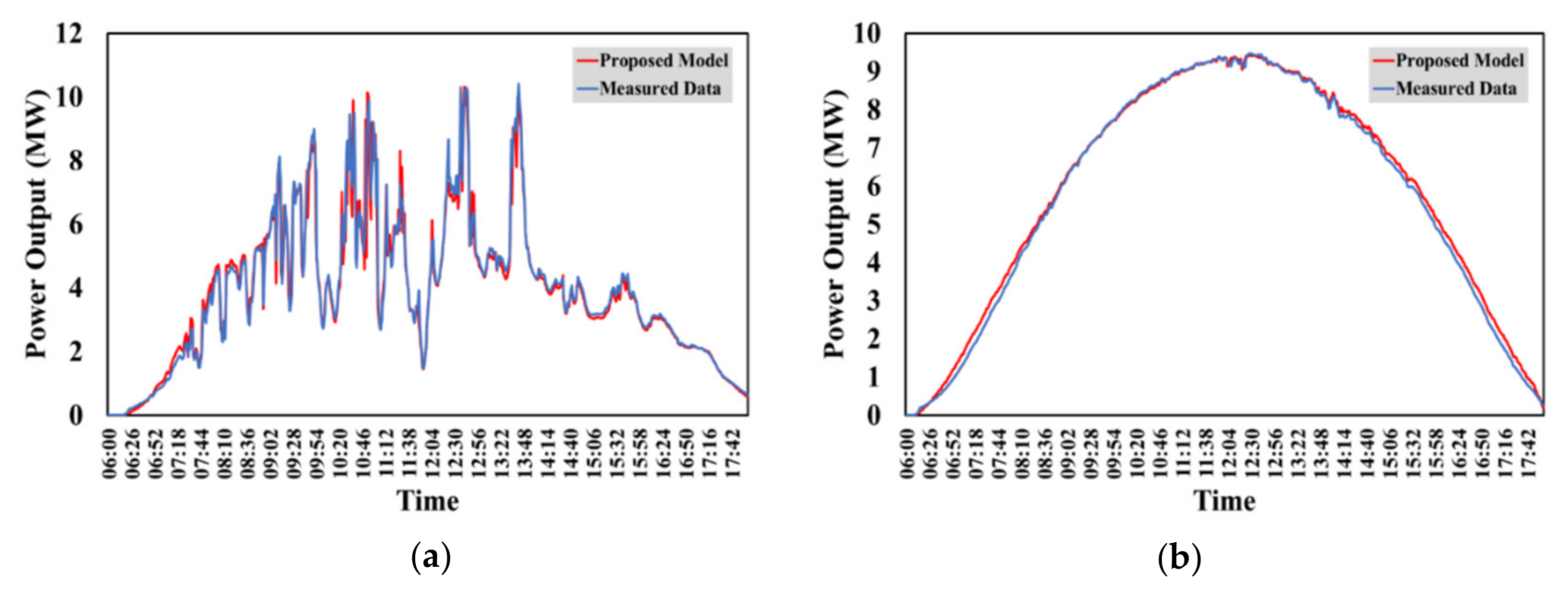
In order to verify the accuracy of the proposed model with the application to the PV system simulation model, the testing and comparison of the simulation results with the actual measurement data can be divided into two conditions. These are the daily PV power output in two weather conditions (cloudy day and sunny day) and the effect of climate change for the electricity production of the photovoltaic systems. In this study, the model was designed to calculate the PV power output in different weather conditions, which are divided into seasons. These are in the summer (February–May), the rainy season (June–September), and the winter (October–January). The division of the seasons in Thailand was taken from the Thai Meteorological Department. The test uses data from photovoltaic systems in Thailand (2018–2019). In order to verify the model that was used to improve the accuracy, the most accurate results to compare the % RMSE [22] values with the measured data is given by

$$\%RMSE=\sqrt{\frac{1}{n}{\displaystyle \sum }_{i=1}^n{\left(\frac{simulat{e}_i-measure{d}_i}{\overline{measured}}\right)}^2}\times 100$$

(40)

where $simulat{e}_i$ is the simulation data, $measure{d}_i$ is the measured data and $\overline{measured}$ is the average value of the measured data.

4.2. Daily PV System Simulation

Figure 13 shows a comparison of the PV power output between the proposed model and the actual measurement data of two weather conditions. The test results are as follows.

The PV power output of the proposed model tends to be in the same direction as the data from the actual measurement data on a cloudy day. This shows that this model can accurately simulate the PV power output in spite of sudden climate change. The nRMSE (normalized RMSE) is deficient (3.19%), as shown in Figure 13a.

The proposed model can accurately simulate the PV power output on a sunny day, and is very useful on days with the right weather conditions. The nRMSE (normalized RMSE) is lower than the cloudy day (1.79%), as shown in Figure 13b.

The PV power output of the proposed model and the actual measurement data are summarized in

Table 7. Comparison of the results on a sunny day and a cloudy day.

Case Day	Measured Data (MW)	Proposed Model (MW)	nRMSE (Normalized RMSE)
Sunny Day	71.43	72.70	1.79
Cloudy Day	64.57	66.63	3.19

. The nRMSE (normalized RMSE) shows the accuracy of the proposed model.

4.3. Seasonal PV System Simulation

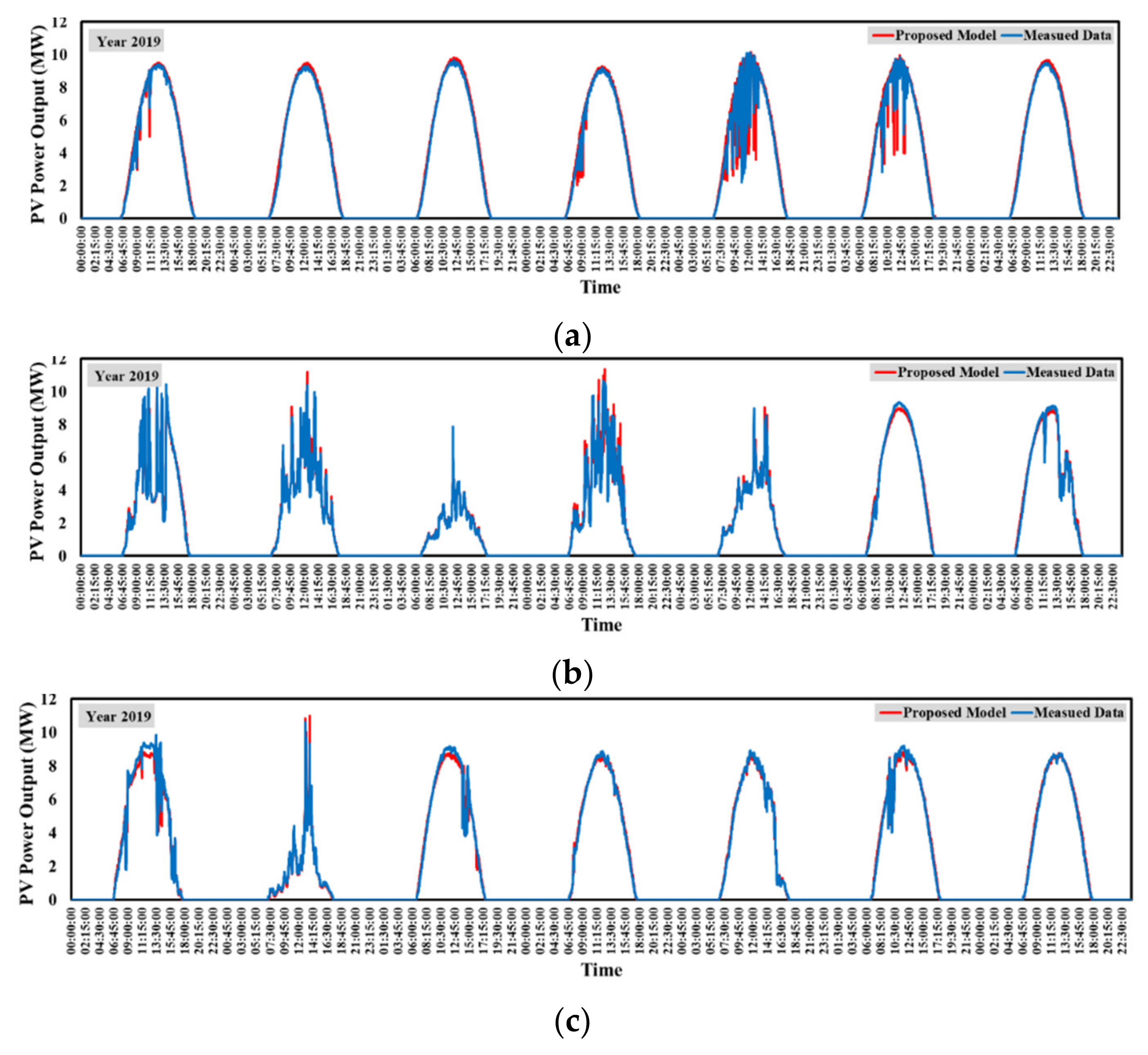
In order to compare the electricity generation data of the proposed model and the actual measurement, the conditions are divided into three seasons: the summer, the rainy season, and the winter. The climate in each season is different. The climate is an essential variable for the electricity generation of the PV system, including solar irradiance, ambient temperature, and module temperature, etc. In this research, the proposed model’s accuracy is checked with the PV system simulation model application that calculates the PV system’s electricity generation in all climatic conditions. In the test, this research randomly generated electricity for one week of the three seasons in 2019.

Figure 14 compares the PV power output between the proposed model and the actual measurement data for the random week of the different seasons. The simulation results of the sampling of the photovoltaic system’s electricity production, the simulation results, and the data from the actual measurements tend to show a similar trend. The daily electricity generation data for all three seasons have different weather conditions. However, the proposed model shows that this model can accurately simulate the electricity production in the different weather conditions.

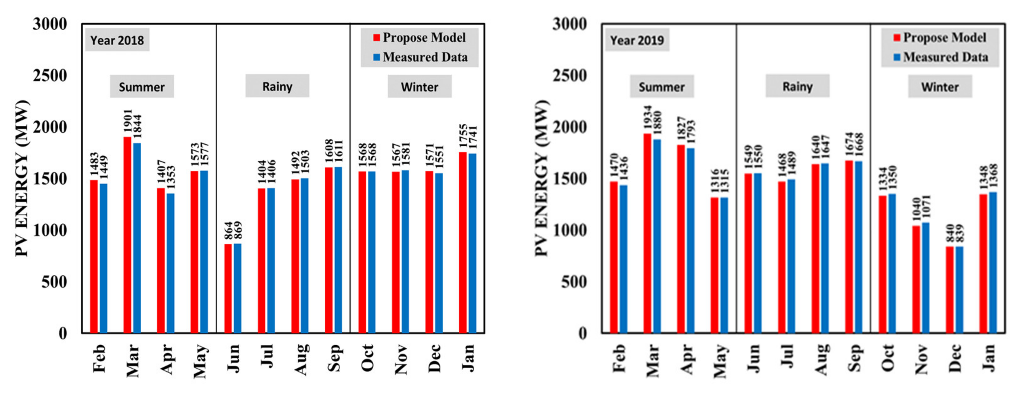
The accuracy of the proposed model of the monthly PV energy simulation compared with the actual measurement data in 2018 and 2019. When analyzing the simulation results of each season, such as in the summer, the rainy season, and the winter in Thailand’s tropical climate, the proposed model can simulate the PV energy precisely in all weather conditions, as shown in Figure 15.

Table 8. Comparison of the results of the proposed model and the measured data in 2018–2019.

Data	2018				2019				2018–2019
	Summer	Rainy	Winter	Average	Summer	Rainy	Winter	Average	Average
Measured Data (MW)	1556	1347	1610	1504	1606	1589	1157	1450	1477
Proposed Model (MW)	1591	1342	1615	1516	1637	1583	1141	1453	1485
nRMSE (Normalized RMSE)	2.43	0.39	0.75	1.19	1.81	0.59	1.40	1.26	1.23

shows the proposed model of the monthly PV energy and the actual measurement data (2018). The proposed model results from 12 months of PV energy in Thailand, showing that the average PV energy is 1516 MWh/month, and the PV energy is 18193 MWh/year. The actual measurement data has an average PV energy of 1504 MWh/month, and PV energy of 18053 MWh/year. The nRMSE (normalized RMSE) ranges from 0.06% to 4.05%, which is very low. The average nRMSE (normalized RMSE) is 1.19% for 12 months (2018).

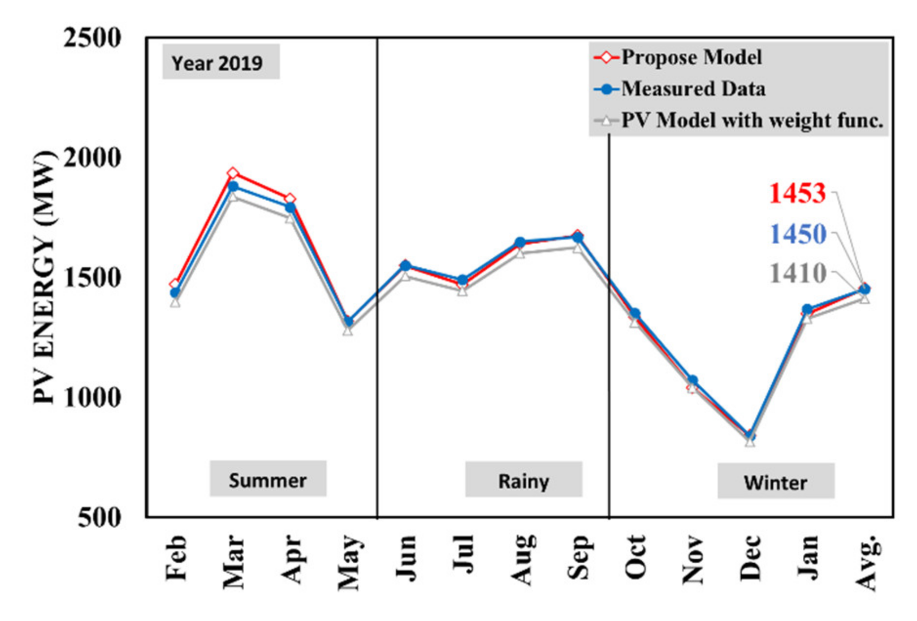
The test results of the PV energy of the proposed model and the actual measurement data on monthly basis (2019) showed that the average PV energy is 1453 MWh/month, and that the PV energy is 17440 MWh/year. The average PV energy is 1450 MWh/month, and the PV energy is 17406 MWh/year in the actual measurement data. The nRMSE (normalized RMSE) ranges from 0.07% to 2.91%, which shows that this value is deficient. The average nRMSE (normalized RMSE) is 1.26% for 12 months (in 2019).

In the comparison of the PV energy of the 24 months data of the proposed model (2018–2019) with the actual measurements for all three seasons, the average nRMSE (normalized RMSE) is 2.12% in the summer, 0.49% in the rainy season, and 1.08% in the winter. These are the results of the proposed model.

In the rainy season, the model is at its highest accuracy. We found that the solar cells in this area performed at their best because the dust was washed off the front of the solar panels by the rain, and because the temperature accumulation of the solar panels is not as high as it is in the summer. Because of this, it causes relatively little energy loss.

In the winter, the model is less accurate than it is in the rainy season, but more accurate than it is in the summer because there is a lot of dust on the front of the solar panel, which is a waste of energy for the solar cells. However, no heat is accumulated on the solar cells; thus, the models presented can be processed better than those in summer.

In the summer, the model is less accurate than both seasons because the summer temperature is high. The heat accumulation of the solar panel causes the temperature to rise.

In the actual case of a solar farm, the panel cleaning is not performed every day, but there is a cleaning cycle. Therefore, the accumulated dust affects the solar cell’s electrical power generation efficiency.

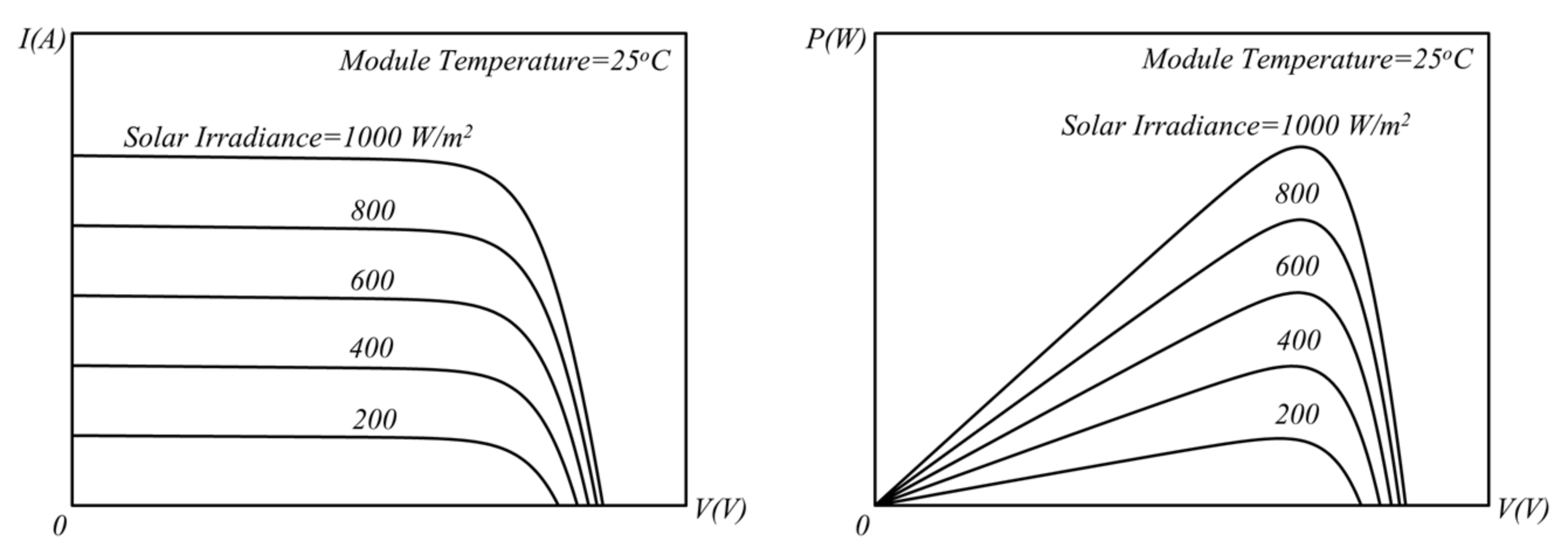
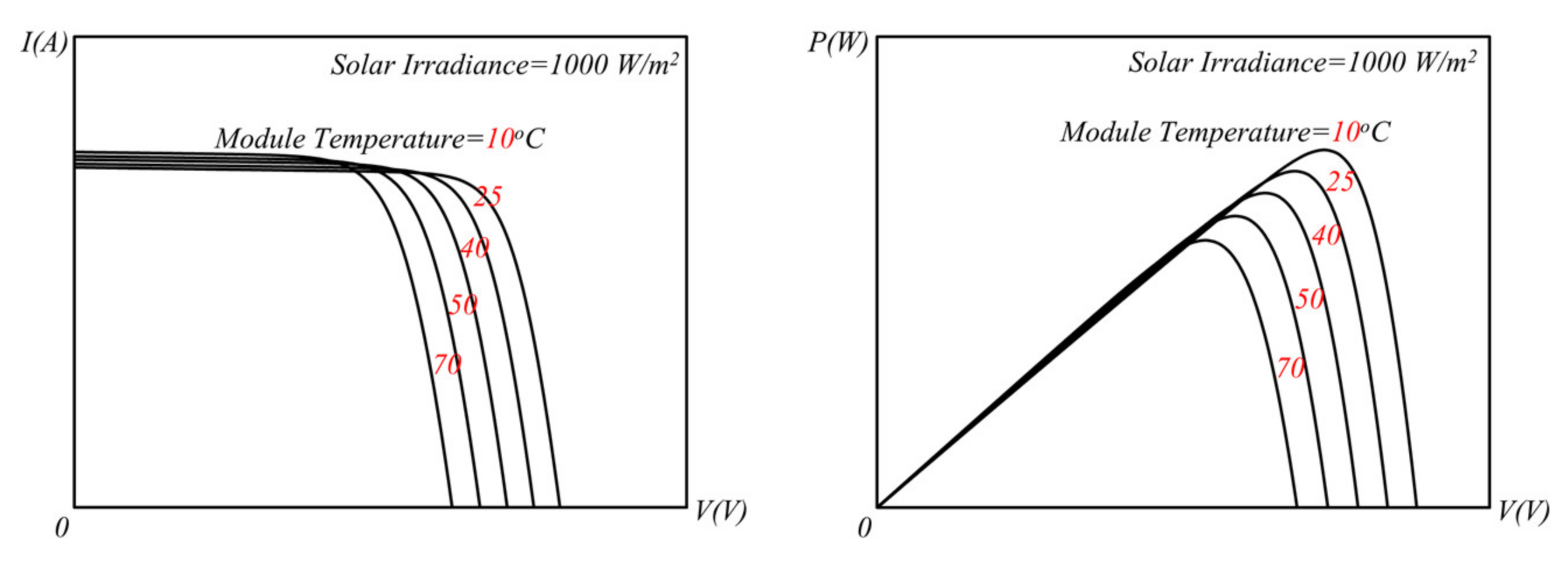
The main factors that affect the PV system’s electricity production are solar irradiance, which varies according to the solar cell’s current, and the panel’s temperature, which varies according to the voltage of the solar cell. The proposed model has a method that uses the relationship of solar irradiance and electricity generation to help improve the accuracy process, but the module temperature is not used as a parameter in this model. For this reason, the accuracy of the model in the summer is lower than it is in the rainy season.

4.4. Comparison with the PV Model with the Weight Function

The precision of the proposed model was verified by the comparison with the PV Model with the weight function [1] and the actual data from the one-year measured data, as shown in Figure 16.

The PV Model with the weight function [1] uses a method to quantify the difference between the simulated data and the actual measurement data in the polynomial equation form in order to improve the simulated data’s accuracy. This method is accurate with a significant increase in the database, but as the database becomes more diffused, the accuracy of this method is lower.

On the other hand, the proposed model was designed to analyze various database behaviors diffused as equations in different forms of ‘curve-fitting process’. The proposed model is a learning model that increases in accuracy every time it analyses and calculates data.

The results show that the proposed model has very high accuracy. The proposed model has a lower nRMSE than the PV Model with the weight function in all three seasons, as shown in

Table 9. Comparison of the proposed model and the PV Model with the weight function in 2019.

Data	Proposed Model				PV Model with Weight Func.
	Summer	Rainy	Winter	Average	Summer	Rainy	Winter	Average
Measured Data (MW)	1606	1589	1157	1450	1606	1589	1157	1450
Simulation Data (MW)	1637	1583	1141	1453	1564	1543	1124	1410
nRMSE (Normalized RMSE)	1.81	0.59	1.40	1.26	2.63	2.89	2.88	2.80

.

5. Conclusions

This research presents a simulation of a method to improve the accuracy of mathematical models (the Preciseness Function Learning Model (PFL Model)) using a PV simulation model of the PV system, a precision test of the model, and a comparison of the 2-year data of the proposed model with the actual measurements of the PV system. The accuracy depends on the function selected from the curve-fitting process.

The results show that the proposed model has the highest accuracy in the rainy season. The average nRMSE (normalized RMSE) of the proposed model is very low (1.23%), and it ranges from 0.30% to 2.26%. It has been proven that this model is very accurate. The proposed model is a learning model that can optimize the higher precision with which the proposed model performs. It can be said that, after the accuracy improvement, the PV power output will be added to the proposed model database in order to enable the model to learn and improve the accuracy of the data in the next prediction results. In the future, we plan to develop models to improve the data accuracy by correlating more than one input to the outputs, in order to reduce the loss or error from the calculation during the data precision improvement.

References

1. Kittisontirak, S.; Bupi, A.; Chinnavornrungsee, P.; Sriprapha, K.; Thajchayapong, P.; Titiroongruang, W. An Improved PV Output Forecasting Model by Using Weight Function: A Case Study in Cambodia. Int. J. Photoenergy 2016, 2016, 1–10. [Google Scholar] [CrossRef] [Green Version]
2. Li, P.; Zhou, K.; Lu, X.; Yang, S. A hybrid deep learning model for short-term PV power forecasting. Appl. Energy 2020, 259, 114216. [Google Scholar] [CrossRef]
3. Guifang, G. Modeling of solar photovoltaic cells and output characteristic simulation based on Simulink. J. Chem. Pharm. Res. 2014, 6, 1791–1795. [Google Scholar]
4. De Soto, W.; Klein, S.A.; Beckman, W. Improvement and validation of a model for photovoltaic array performance. Sol. Energy 2006, 80, 78–88. [Google Scholar] [CrossRef]
5. Karatepe, E.; Boztepe, M.; Colak, M. Neural network based solar cell model. Energy Convers. Manag. 2006, 47, 1159–1178. [Google Scholar] [CrossRef]
6. Brano, V.L.; Orioli, A.; Ciulla, G.; Di Gangi, A. An improved five-parameter model for photovoltaic modules. Sol. Energy Mater. Sol. Cells 2010, 94, 1358–1370. [Google Scholar] [CrossRef]
7. Bupi, A.; Kittisontirak, S.; Sriprapha, K.; Siriwongrungsan, W.; Titiroongruang, W.; Niemcharoen, S. A simplified model for the estimation of energy production of PV module. In Proceedings of the 2017 International Electrical Engineering Congress (iEECON), Pattaya, Thailand, 8–10 March 2017. [Google Scholar]
8. Bupi, A.; Kittisontirak, S.; Sriprapha, K.; Siriwongrungsan, W.; Titiroongruang, W.; Niemcharoen, S. Comparison of PV module power output measurements. In Proceedings of the 2017 International Electrical Engineering Congress (iEECON), Pattaya, Thailand, 8–10 March 2017. [Google Scholar]
9. Vinod; Kumar, R.; Singh, S.K. Solar photovoltaic modeling and simulation: As a renewable energy solution. Energy 2018, 4, 701–712. [Google Scholar] [CrossRef]
10. Maninder Kaur, E. Simulation Model for PV Array & its Characteristics. Int. J. Electr. Eng. Educ. 2014, 1, 1694–2426. [Google Scholar]
11. Tsai, H.L. Insolation-oriented model of photovoltaic module using Matlab/Simulink. Sol. Energy 2010, 84, 1318–1326. [Google Scholar] [CrossRef]
12. Altas, I.H.; Sharaf, A.M. A photovoltaic array simulation model for Matlab-Simulink GUI environment. In Proceedings of the International Conference on Clean Electrical Power, Capri, Italy, 21–23 May 2007; pp. 341–345. [Google Scholar]
13. Vengatesh, R.P.; Rajan, S.E. Investigation of cloudless solar radiation with PV module employing Matlab-Simulink. In Proceedings of the International Conference on Emerging Trends in Electrical and Computer Technology, Nagercoil, India, 23–24 March 2011; pp. 141–147. [Google Scholar]
14. Maffezzoni, P.; Codecasa, L.; D’Amore, D. Modeling and Simulation of a Hybrid Photovoltaic Module Equipped with a Heat-Recovery System. IEEE Trans. Ind. Electron. 2009, 56, 4311–4318. [Google Scholar] [CrossRef]
15. Pandiarajan, N.; Muthu, R. Mathematical modeling of a photovoltaic module with Simulink. In Proceedings of the International Conference on Electrical Energy Systems, Chennai, India, 3–5 January 2011; pp. 258–263. [Google Scholar]
16. Rustemli, S.; Dincer, F. Modeling of Photovoltaic Panel and Examining Effects of Temperature in Matlab/Simulink. Electron. Electr. Eng. 2011, 3, 35–40. [Google Scholar] [CrossRef] [Green Version]
17. Nema, S.; Nema, R.K.; Agnihotri, G. MATLAB/Simulink based study of photovoltaic cells/modules/array and their experimental verification. Int. J. Energy Environ. 2010, 1, 487–500. [Google Scholar]
18. Bellia, H.; Youcef, R.; Fatima, M. A detailed modeling of photovoltaic module using MATLAB/SIMULINK. J. Astron. Geophys. 2014, 3, 53–61. [Google Scholar] [CrossRef] [Green Version]
19. Levy, E.C. Complex-curve fitting. IRE Trans. Automatic Control 1959, AC-4, 37–43. [Google Scholar] [CrossRef]
20. O’Hagan, A. Curve Fitting and Optimal Design for Prediction. J. R. Stat. Soc. Ser. B Methodol. 1978, 40, 1–24. [Google Scholar]
21. McIntosh, K.R.; Honsberg, C.B. The Influence of Edge Recombination on a Solar Cell’s IV Curve. In Proceedings of the 16th Euro-pean Photovoltaic Solar Energy Conference, Glasgow, UK, 1–5 May 2000. [Google Scholar]
22. Chai, T.; Draxler, R.R. Root mean square error (RMSE) or mean absolute error (MAE)? Arguments against avoiding RMSE in the literature. Geosci. Model Dev. 2014, 7, 1247–1250. [Google Scholar] [CrossRef] [Green Version]
Figure 1. Ideal single diode equivalent circuit of a photovoltaic cell [7,8].
Energies 14 00372 g001
Figure 2. Electrical properties of the solar cells when exposed to solar irradiance.
Energies 14 00372 g002
Figure 3. Equivalent circuit (Single diode) of a photovoltaic cell [7,8].
Energies 14 00372 g003
Figure 4. Influence of the series resistance on the solar cell output properties.
Energies 14 00372 g004
Figure 5. Effect of solar irradiance on the solar cells [7,8].
Energies 14 00372 g005
Figure 6. Effect of temperature on the solar cells [7,8].
Energies 14 00372 g006
Figure 7. Structure of the Preciseness Function Learning Model (PFL Model).
Energies 14 00372 g007
Figure 8. Example of a database of the model with curve-fitting in various forms.
Energies 14 00372 g008
Figure 9. Learning method structure of the preciseness function learning model (PFL Model).
Energies 14 00372 g009
Figure 10. Structure of the photovoltaic simulation model with preciseness function learning model (PFL model).
Energies 14 00372 g010
Figure 11. Accuracy improvement of the proposed model.
Energies 14 00372 g011
Figure 12. Simulation result of the accuracy improvement.
Energies 14 00372 g012
Figure 13. The proposed model and the measured data of the PV power output on a cloudy day (a) and a sunny day (b).
Energies 14 00372 g013
Figure 14. The proposed model and the measured data of the PV power output in the three seasons. (a) In the summer; (b) in the rainy season; (c) in the winter.
Energies 14 00372 g014
Figure 15. Comparison of the PV energy of the simulated and measured data of the different seasons.
Energies 14 00372 g015
Figure 16. Comparison of the PV energy of the simulated and measured data of the different seasons.
Energies 14 00372 g016