
Feature Extraction, Ageing Modelling and Information Analysis of a Large-Scale Battery Ageing Experiment


Abstract
: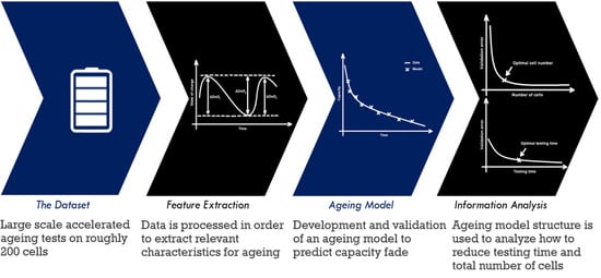
1. Introduction
2. Battery Ageing Data
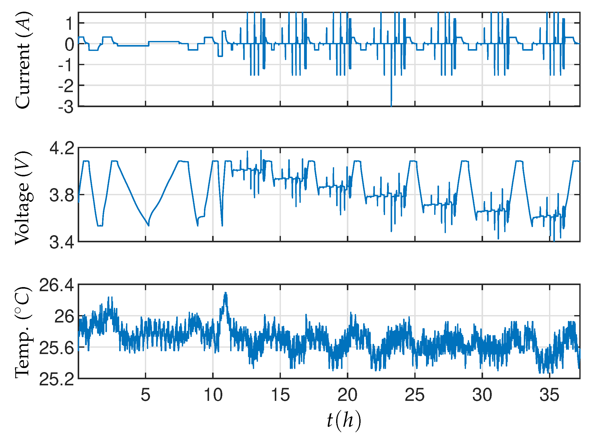
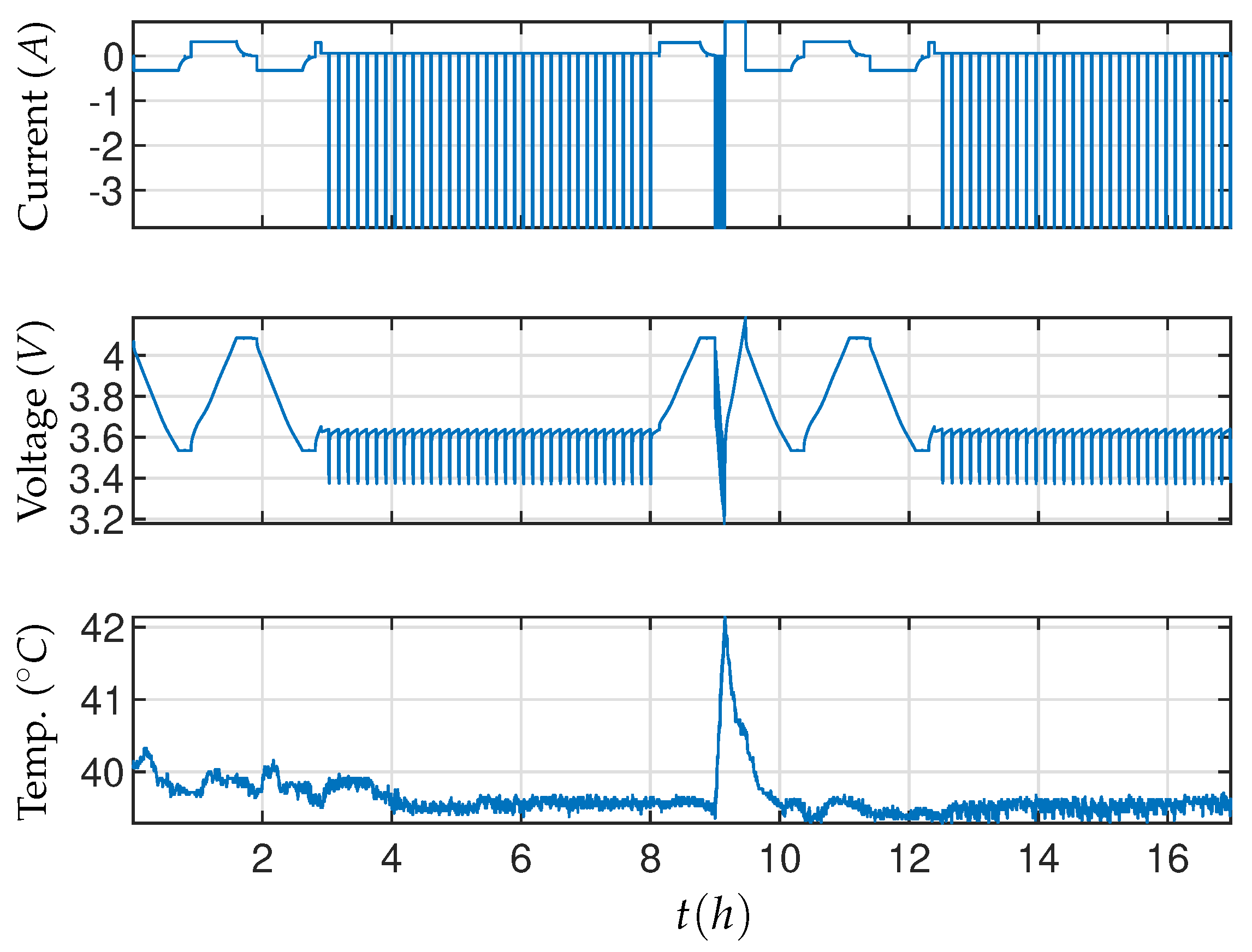
2.1. Dataset Description and Testing Equipment
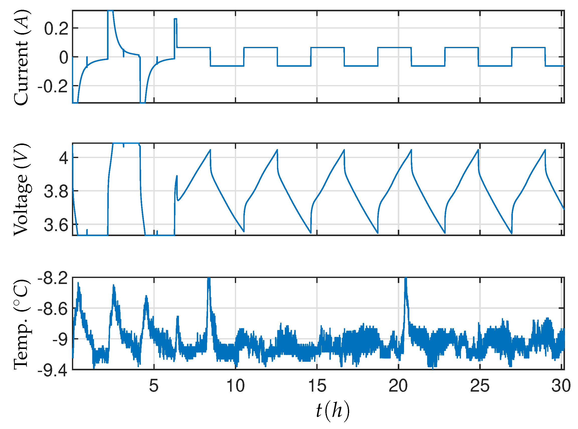
2.2. Testing Overview
2.3. Capacity Estimation and Initial Analysis
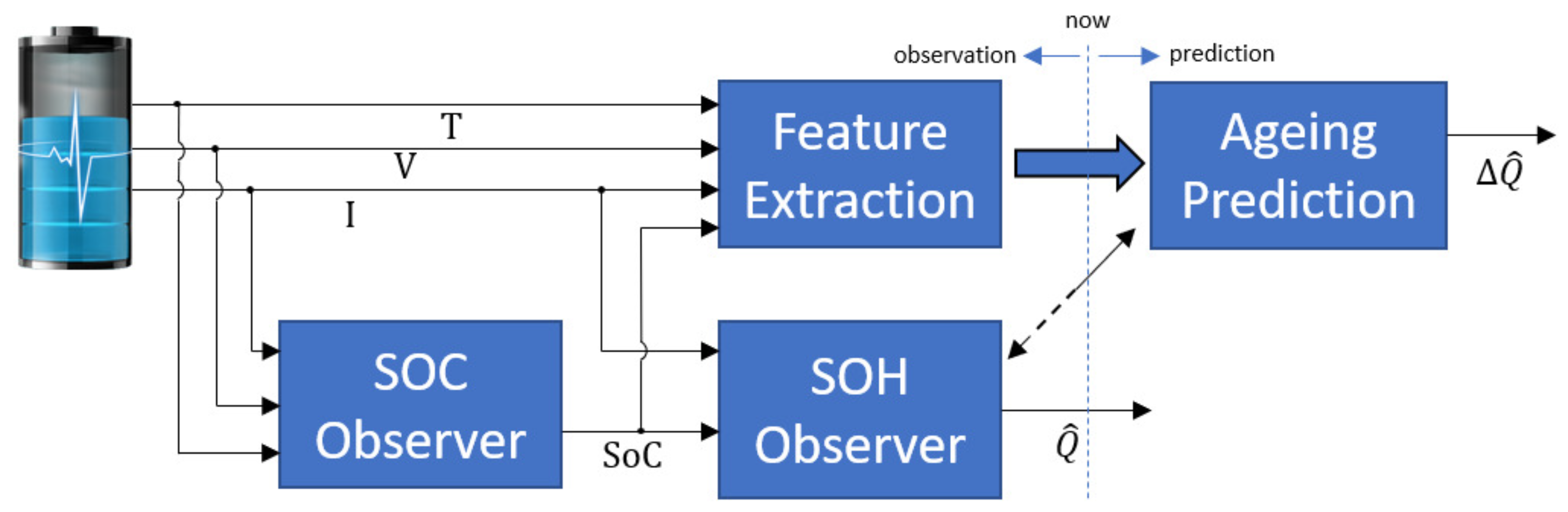
3. Model Based Analysis
4. Model Structure Selection
4.1. Structure Considerations
- Given an arbitrary with elapsed time and charge throughput , if we split the interval into parts such that:thenmust hold for any positive , , , .
- If and are zero then . Note that it is not possible that and .
- In [7], the ageing effects were described together with accelerating factors. One possible way to take that into consideration is that these accelerating factors should be linked to a main ageing feature in a regression structure.
- Ideally, the model’s structure should be kept simple in order to, if necessary, perform the parametrisation in an online fashion, with limited hardware, such as in a BMS.
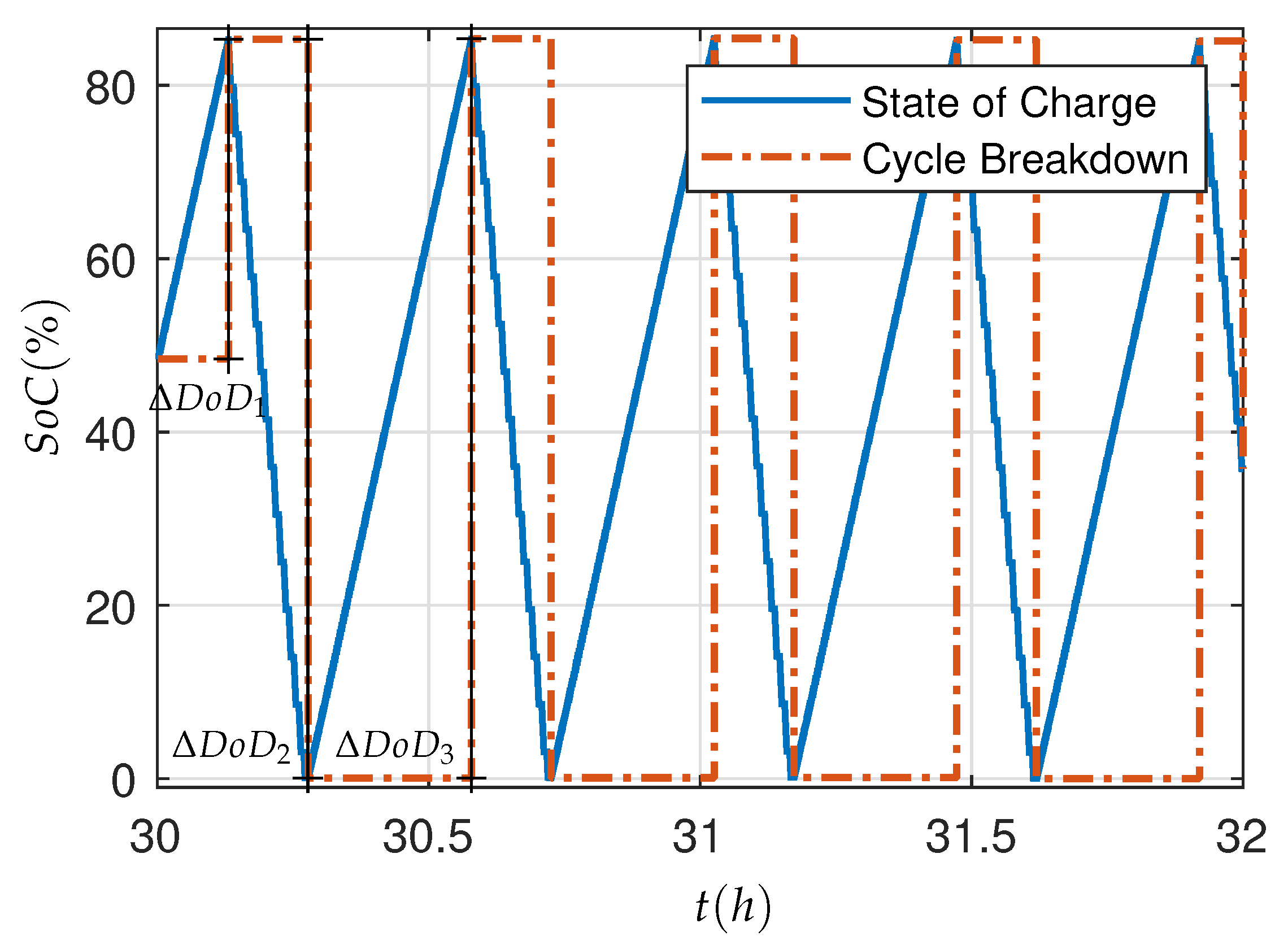
4.2. Feature Selection
5. Model Training and Validation
6. Information Analysis
- How much data and testing time are needed in order to parametrize the model?
- How much of the dataset and how much testing time would have been needed to sufficiently parametrize the model?
6.1. Fisher Information
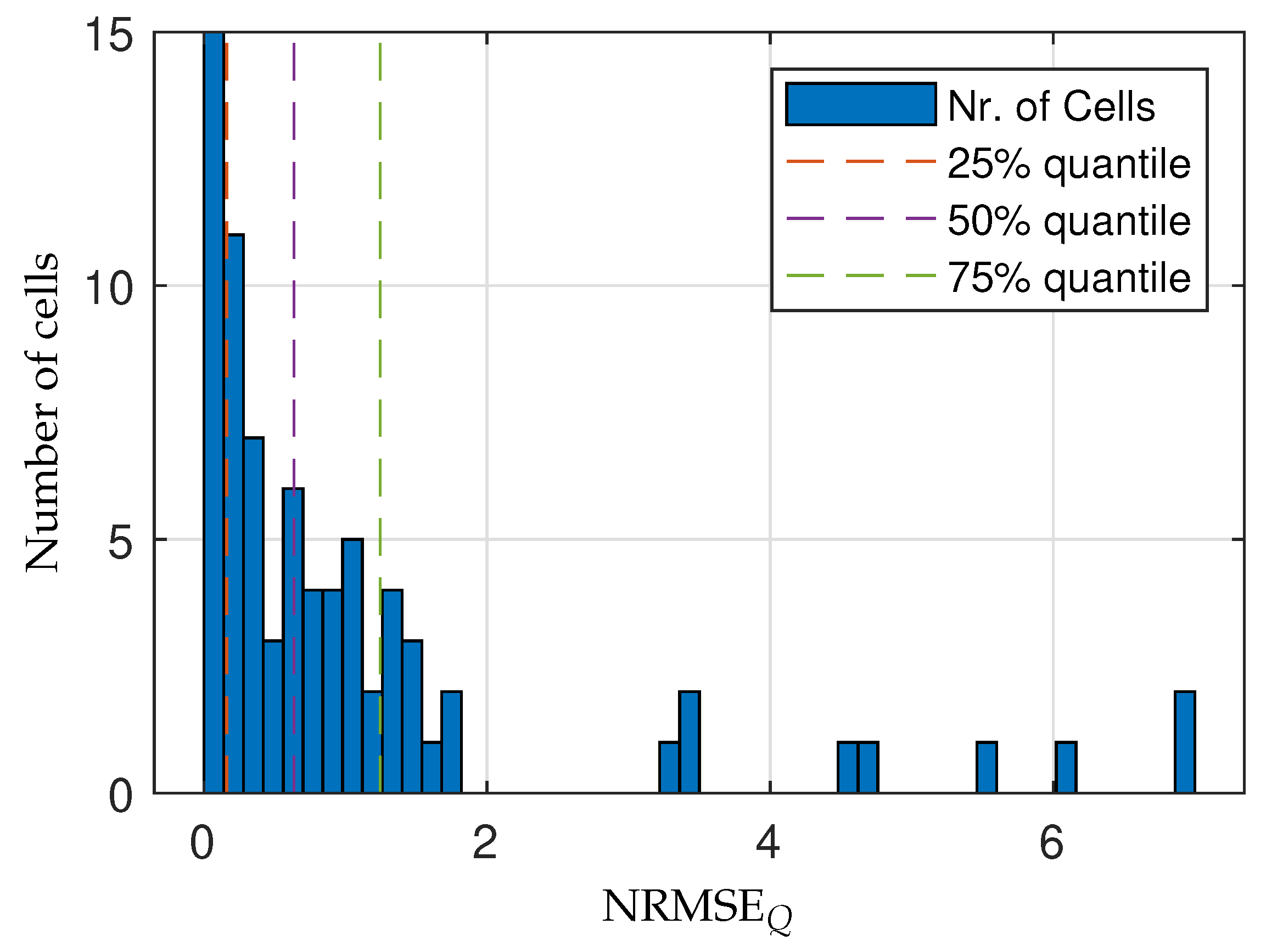
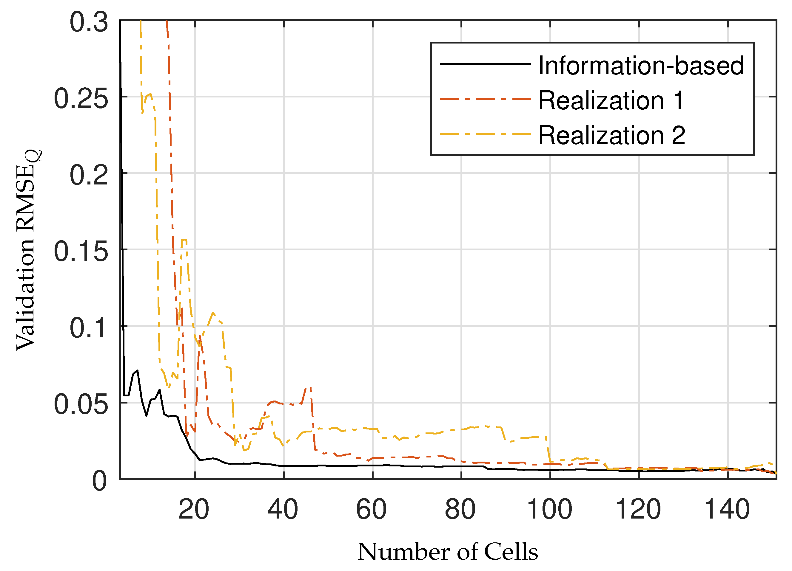
6.2. Optimal Cell Selection
6.3. Impact of the Testing Time
7. Conclusions
Author Contributions
Funding
Institutional Review Board Statement
Informed Consent Statement
Data Availability Statement
Conflicts of Interest
References
- Lutsey, N.; Nicholas, M. Update on electric vehicle costs in the United States through 2030. Int. Counc. Clean Transp. 2019, 9. [Google Scholar]
- Hoke, A.; Brissette, A.; Smith, K.; Pratt, A.; Maksimovic, D. Accounting for Lithium-Ion Battery Degradation in Electric Vehicle Charging Optimization. IEEE J. Emerg. Sel. Top. Power Electron. 2014, 2, 691–700. [Google Scholar] [CrossRef]
- Plett, G.L. Sigma-point Kalman filtering for battery management systems of LiPB-based HEV battery packs: Part 2: Simultaneous state and parameter estimation. J. Power Sources 2006, 161, 1369–1384. [Google Scholar] [CrossRef]
- Hametner, C.; Jakubek, S.; Prochazka, W. Data-Driven Design of a Cascaded Observer for Battery State of Health Estimation. IEEE Trans. Ind. Appl. 2018, 54, 6258–6266. [Google Scholar] [CrossRef]
- Chen, C.; Xiong, R.; Shen, W. A Lithium-Ion Battery-in-the-Loop Approach to Test and Validate Multiscale Dual H Infinity Filters for State-of-Charge and Capacity Estimation. IEEE Trans. Power Electron. 2018, 33, 332–342. [Google Scholar] [CrossRef]
- Hu, X.; Xu, L.; Lin, X.; Pecht, M. Battery Lifetime Prognostics. Joule 2020, 4, 310–346. [Google Scholar] [CrossRef]
- Vetter, J.; Novák, P.; Wagner, M.; Veit, C.; Moller, K.C.; Besenhard, J.; Winter, M.; Wohlfahrt-Mehrens, M.; Vogler, C.; Hammouche, A. Ageing mechanisms in lithium-ion batteries. J. Power Sources 2005, 147, 269–281. [Google Scholar] [CrossRef]
- Ramadass, P.; Haran, B.; Gomadam, P.M.; White, R.; Popov, B.N. Development of First Principles Capacity Fade Model for Li-Ion Cells. J. Electrochem. Soc. 2004, 151, A196–A203. [Google Scholar] [CrossRef]
- Jin, X.; Vora, A.; Hoshing, V.; Saha, T.; Shaver, G.; García, R.E.; Wasynczuk, O.; Varigonda, S. Physically-based reduced-order capacity loss model for graphite anodes in Li-ion battery cells. J. Power Sources 2017, 342, 750–761. [Google Scholar] [CrossRef] [Green Version]
- Wang, J.; Liu, P.; Hicks-Garner, J.; Sherman, E.; Soukiazian, S.; Verbrugge, M.; Tataria, H.; Musser, J.; Finamore, P. Cycle-life model for graphite-LiFePO4 cells. J. Power Sources 2011, 196, 3942–3948. [Google Scholar] [CrossRef]
- Schmalstieg, J.; Käbitz, S.; Ecker, M.; Sauer, D.U. A holistic aging model for Li(NiMnCo)O2 based 18650 lithium-ion batteries. J. Power Sources 2014, 257, 325–334. [Google Scholar] [CrossRef]
- Richardson, R.R.; Osborne, M.A.; Howey, D.A. Battery health prediction under generalized conditions using a Gaussian process transition model. J. Energy Storage 2019, 23, 320–328. [Google Scholar] [CrossRef]
- Wu, X.; Li, X.; Du, J. State of Charge Estimation of Lithium-Ion Batteries Over Wide Temperature Range Using Unscented Kalman Filter. IEEE Access 2018, 6, 41993–42003. [Google Scholar] [CrossRef]
- Hametner, C.; Jakubek, S. State of charge estimation for Lithium Ion cells: Design of experiments, nonlinear identification and fuzzy observer design. J. Power Sources 2013, 238, 413–421. [Google Scholar] [CrossRef]
- Santhanagopalan, S.; Smith, K.; Neubauer, J.; Kim, G.H.; Keyser, M.; Pesaran, A. Design and aNalysis of Large Lithium-Ion Battery Systems, 1st ed.; Artech House: Norwood, MA, USA, 2015; Volume 4. [Google Scholar]
- Friedman, H.; Tibshirani. The Elements of Statistical Learning, 2nd ed.; Springer: Berlin/Heidelberg, Germany, 2008. [Google Scholar]
- Ferreira, A.J.; Figueiredo, M.A. Efficient feature selection filters for high-dimensional data. Pattern Recognit. Lett. 2012, 33, 1794–1804. [Google Scholar] [CrossRef] [Green Version]
- Liu, H.; Motoda, H. Feature Selection for Knowledge Discovery and Data Mining, 1st ed.; Springer: New York City, NY, USA, 1998. [Google Scholar]
- Boyd, S.; Vandenberghe, L. Convex Optimization, 7th ed.; Cambridge University Press: Cambridge, UK, 2009. [Google Scholar]
- Davison, A.C. Statistical Models, 1st ed.; Cambridge University Press: Cambridge, UK, 2003. [Google Scholar]


| Cell Chemistry | |
| Positive Electrode | NMC |
| Negative Electrode | Graphite |
| Nominal Capacity | 330 mAh |
| Upper Voltage Limits | |
| Constant Current | 4.085 V |
| 5 s Pulse | 4.2 V |
| Safety Limit | 4.5 V |
| Lower Voltage Limits | |
| Constant Current | 3.354 V |
| 5 s Pulse | 2.8 V |
| Safety Limit | 2.5 V |
| Variable | Minimum | Maximum |
|---|---|---|
| T | −20 °C | 45 °C |
| CC | 0.2 °C | 2.4 °C |
| PDC | 0.2 °C | 10 °C |
| SOC | 15% | 80% |
| dDoD | 2.5% | 80% |
| Cell Nr. | Temperature | Duration | Mean Ah | Total Ah | Initial Cap. | Cap. Loss |
|---|---|---|---|---|---|---|
| 1 | −9 | 540 | 1.33 | 2.83 | 315 | 33 |
| 4 | 8 | 546 | 1.27 | 2.93 | 314 | 40 |
| 5 | 8 | 310 | 9.83 | 7.20 | 329 | 115 |
| 17 | 8 | 395 | 1.47 | 2.84 | 321 | 38 |
| 33 | 41 | 546 | 1.20 | 2.28 | 319 | 69 |
| 46 | −8 | 148 | 1.33 | 3.62 | 320 | 65 |
| 63 | 29 | 547 | 1.55 | 4.06 | 322 | 35 |
| 141 | 40 | 418 | 1.24 | 3.50 | 324 | 96 |
| 217 | 42 | 176 | 1.10 | 9.62 | 319 | 120 |
| Feature | Description |
|---|---|
| Time interval | |
| Charge in a given interval | |
| T | Average temperature |
| Absolute time at the beginning | |
| Absolute total charge at the beginning | |
| Average Voltage | |
| Average | |
| Average cycle magnitude extracted from | |
| Same as above, but extracted from Current I | |
| Cycling frequency extracted from | |
| Same as above, but extracted from Current I | |
| Average charging current | |
| Average discharging current | |
| Average squared current | |
| Sum of squared current | |
| N | Number of cycles from analysis |
| Dataset | ||
|---|---|---|
| Training Data | 0.0087 | 0.0353 |
| Validation Data | 0.0084 | 0.0384 |
| Dataset | ||
|---|---|---|
| Training Data | 0.0088 | 0.0364 |
| Validation Data | 0.0086 | 0.0395 |
Publisher’s Note: MDPI stays neutral with regard to jurisdictional claims in published maps and institutional affiliations. |
© 2021 by the authors. Licensee MDPI, Basel, Switzerland. This article is an open access article distributed under the terms and conditions of the Creative Commons Attribution (CC BY) license (https://creativecommons.org/licenses/by/4.0/).
Share and Cite
de Oliveira, J.G., Jr.; Dhingra, V.; Hametner, C. Feature Extraction, Ageing Modelling and Information Analysis of a Large-Scale Battery Ageing Experiment. Energies 2021, 14, 5295. https://doi.org/10.3390/en14175295
de Oliveira JG Jr., Dhingra V, Hametner C. Feature Extraction, Ageing Modelling and Information Analysis of a Large-Scale Battery Ageing Experiment. Energies. 2021; 14(17):5295. https://doi.org/10.3390/en14175295
Chicago/Turabian Stylede Oliveira, Jose Genario, Jr., Vipul Dhingra, and Christoph Hametner. 2021. "Feature Extraction, Ageing Modelling and Information Analysis of a Large-Scale Battery Ageing Experiment" Energies 14, no. 17: 5295. https://doi.org/10.3390/en14175295