
Cost-Optimized Heat and Power Supply for Residential Buildings: The Cost-Reducing Effect of Forming Smart Energy Neighborhoods


Abstract
:1. Introduction
- Providing a comprehensive analysis on the circumstances under which SENs are advantageous compared to individually planned buildings.
- The analysis should be detached from specific case studies and take into account key parameters like neighborhood scale, population density, and emissions reduction targets.
2. Methods
2.1. Conception and Experimental Setup
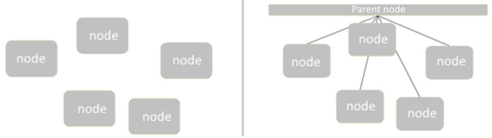
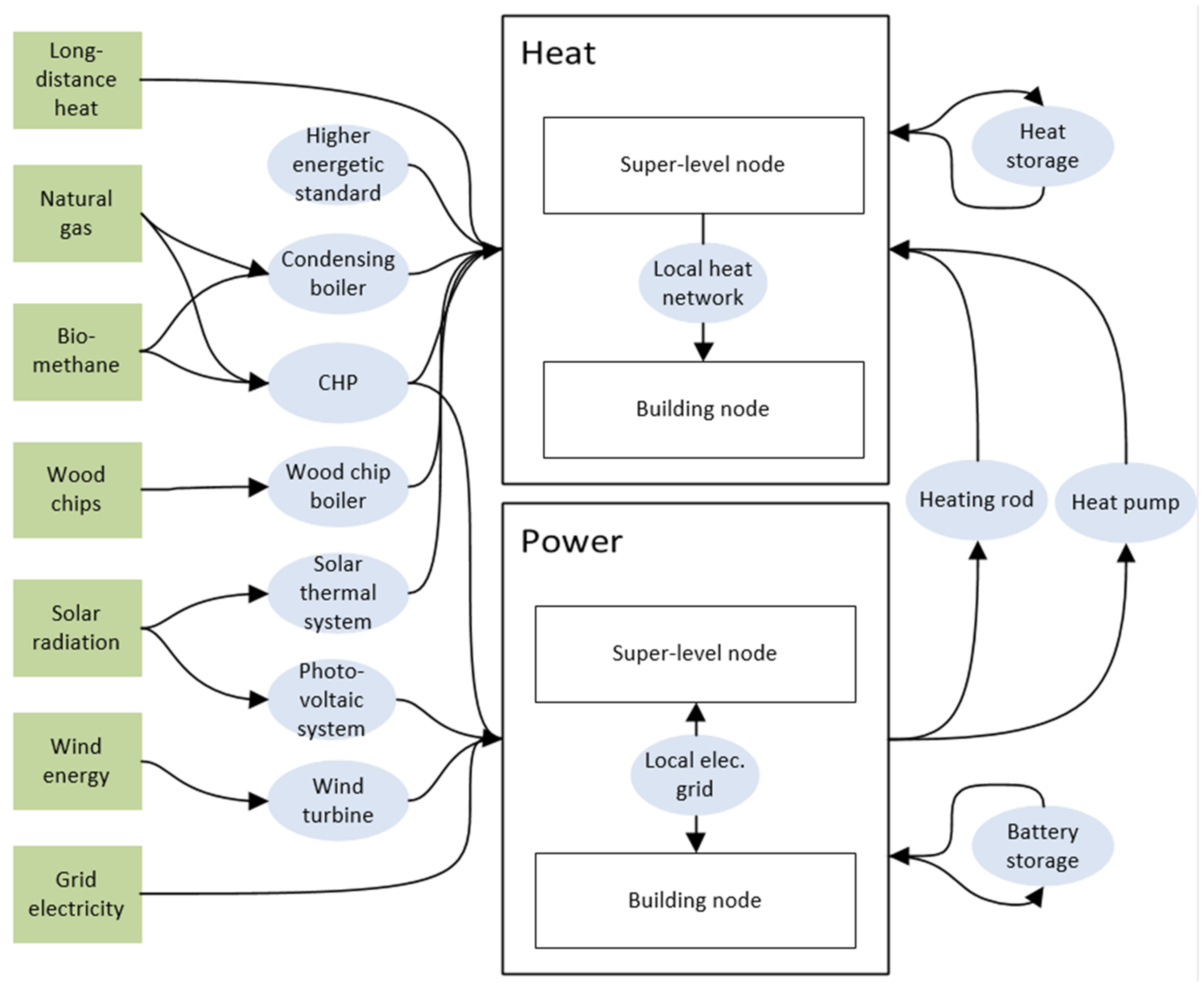
2.2. Modelling Approach
- Aggregation of multiple nodes to one node;
- Time slices to reduce time steps within one year (for the calculations in the results section, 48 representative days are selected).
2.3. Objective Function and Constraints
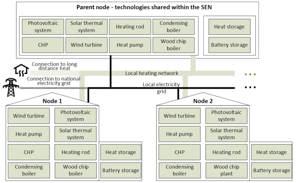
2.4. Considered Pathways and Technologies
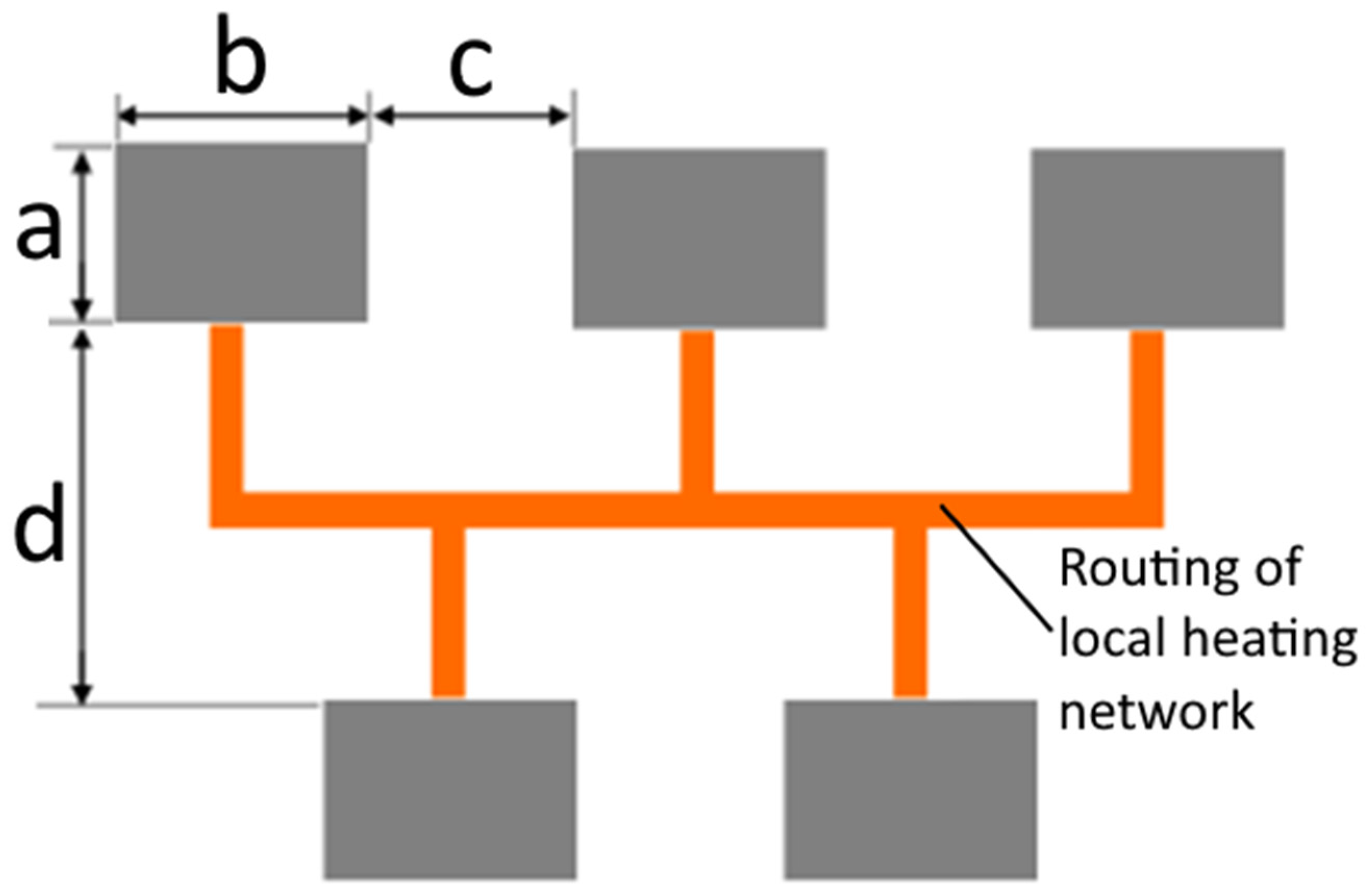
2.5. Variation of Neighborhood Structures
- The building clusters are homogenous, i.e., consist out of identical building types.
- The buildings spread along one axis.
- The spaces between the buildings are regular and occur repeatedly.
2.6. Heating Network
2.7. Potentials of Renewables
2.8. Implementation of Cost-Reducing and Cost-Increasing Effects within SENs
2.9. Demand Profiles
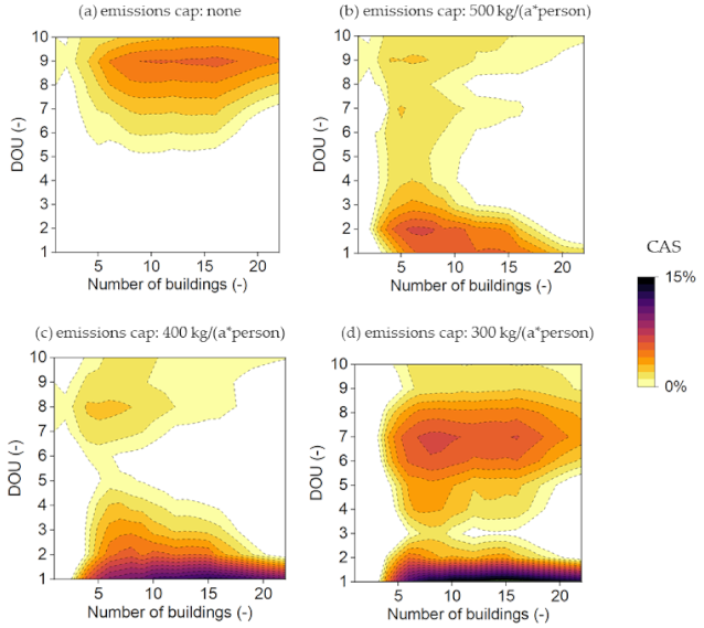
3. Results and Discussion
4. Conclusions
Author Contributions
Funding
Conflicts of Interest
Abbreviations
| SEN | Smart energy neighborhood |
| DOU | Degree of urbanization |
| CAS | Cost advantage of a smart energy neighborhood compared to individually planned buildings |
| CHP | Combined heat and power |
Appendix A

| Energy Form | Price | Emissions Factor | |||
|---|---|---|---|---|---|
| Electricity | Ø 0.130 | (EUR/kWh) | 241 | (g/kWh) | |
| … network tariff: … fluctuating stock price: | 0.079 Ø 0.051 | (EUR/kWh) (EUR/kWh) | |||
| Natural gas | 0.040 | (EUR/kWh) | 240 | (g/kWh) | |
| Biomethane | 0.070 | (EUR/kWh) | 80 | (g/kWh) | |
| Wood chips | 0.0321–0.0442 * | (EUR/kWh) | 16 | (g/kWh) | |
| … of which market price: … of which transport: | 0.030 0.002 1–0.014 2 | (EUR/kWh) (EUR/kWh) | |||
| Long-distance heat | 0.070 2–0.110 1 * | (EUR/kWh) | 79 | (g/kWh) | |
| Feed-in tariff | Ø 0.051 | (EUR/kWh) | |||
| Energy Source | Unit | Value |
|---|---|---|
| Photovoltaic gain | (kWh/kWp *a) | 1029 |
| Solar thermal gain | (kWh/kWth *a) | 2800 |
| Wind turbine gain | (kWh/mrot2 * a) | 702–191 1 * |
| Availability of wood | (kWh/person *a) | 1532–1608 1 * |
| Environmental heat | (kWh/a) | Ꝏ |
| Technology | Unit | Value |
|---|---|---|
| Condensing boiler | (-) | 0.94 |
| CHP plant (<15 kWel) | (-) | 0.254(el); 0.597 (th) |
| CHP plant (>15 kWel) | (-) | 0.305(el); 0.547 (th) |
| Heat pump (air) | (-) | 2.7 |
| Heat pump (ground) | (-) | 3.5 |
| Wood chip boiler | (-) | 0.75 |
| Heating rod | (-) | 0.98 |
| Heat storage | (-) | 0.95 (SL.); 1.00 (char.); 1.00 (dischar.) |
| Battery storage | (-) | 1.00 (SL.); 0.95 (char.); 0.95 (dischar.) |
| Local heating network (2 buildings) | (-) | 0.811–0.96 2 * |
| Tech | Lifetime (a) | O&M (% of Invest) | Fixed Costs (EUR) | Linear Costs (EUR/kW) |
|---|---|---|---|---|
| Photovoltaic system | 20 | 2 | 3240 | 1168 |
| Solar thermal system | 20 | 2 | 2314 | 1041 |
| Heat pump (air) | 20 | 2 | 12,336 | 509 |
| Heat pump (ground) | 20 | 2 | 14,919 | 1339 |
| Wood chip boiler | 20 | 2 | 18,903 | 274 |
| Condensing boiler | 20 | 2 | 8949 | 271 |
| Heating rod | 40 | 2 | 0 | 90 |
| CHP plant (<15 kWel) | 15 | 3 | 15,393 | 2761 |
| CHP plant (>15 kWel) | 15 | 3 | 34,562 | 1254 |
| Heat storage | 40 | 0 | 1697 | 722 |
| Battery storage | 20 | 0 | 800 | 15 |
| DOU | ||||
|---|---|---|---|---|
| 1 | … | 10 | ||
| Building Specific and Demographic Parameters | ||||
| Number of households per building | (-) | 1 | 20 | |
| Persons per household | (-) | 3.0 | 2.0 | |
| Length of building | (m) | 9.0 | 20.0 | |
| Width of building | (m) | 12.0 | 25.0 | |
| Vertical space between buildings | (m) | 20.0 | 2.0 | |
| Horizontal space between buildings | (m) | 30.0 | 20.0 | |
| Number of floors per building | (-) | 2 | 5 | |
| Area (use space) per person | (m2) | 50 | 44 | |
| Demand Parameters | ||||
| Electricity demand | (kWh/a *HH) | 3650 | 2265 | |
| Heat demand | (kWh/a *HH) | 10,395 | 5031 | |
| Specific heat demand (room) | (kWh/a *m 2) | 56 | 45 | |
| Specific heat demand (hot water) | (kWh/a *m 2) | 12.5 | 12.5 | |
| Saving through efficiency measure | (-) | 0.30 | 0.33 | |
| Unit | Value | |
|---|---|---|
| Local heating network (pipes, etc.) | (EUR/m) | 200 1–300 2 * |
| Connection to the local heating network | (EUR/building) | 4254 |
| Electricity network (power lines, etc.) | (EUR/m) | 70 |
| Connection to the electricity network | (EUR/building) | 1100 |
| Total costs of the heating network and local electricity grid: | ||
| (A1) | ||
| (A2) | ||
| C: Total cost c: specific cost l: routing distance n: number of buildings Indexes: hn = heating network; opt = optimal; rout = routing; con = connection; gr = electricity grad | ||

References
- Publications Office of the European Union. Clean Energy for all Europeans. EURATOM Supply Agency—Annual Report 2017. 2019. Available online: https://op.europa.eu/en/publication-detail/-/publication/b4e46873-7528-11e9-9f05-01aa75ed71a1/language-en?WT.mc_id=Searchresult&WT.ria_c=null&WT.ria_f=3608&WT.ria_ev=search (accessed on 12 May 2021).
- Otto, H.; Zöckler, J.-F. EU-Clean Energy Package. Available online:https://www.pwc.de/de/energiewirtschaft/regulierung/eu-clean-energy-package.html (accessed on 19 June 2021).
- European Commission. Energy Communities. Available online:https://ec.europa.eu/energy/topics/markets-and-consumers/energy-communities_en#:~:text=Energy%20communities%20organise%20collective%20and,moving%20citizens%20to%20the%20fore.&text=At%20the%20same%20time%2C%20they,and%20lowering%20their%20electricity%20bills (accessed on 12 May 2021).
- Caramizaru, A.; Uihlein, A. Energy Communities: An Overview of Energy and Social Innovation, Ixelles, Belgium. 2020. Available online: https://www.researchgate.net/profile/Andreas-Uihlein/publication/339676692_Energy_communities_an_overview_of_energy_and_social_innovation/links/5e5f6fe0299bf1bdb850ccbf/Energy-communities-an-overview-of-energy-and-social-innovation.pdf (accessed on 12 May 2021).
- Brassart, M.; Hansen, X.; Henriot, P.; Lacher, E.; Lo Schiavo, L.; Powis, O.; Sidén, J.; Ström, L.; Vögel, S. Regulatory Aspects of Self- Consumption and Energy Communities: Customers and Retail. Markets and Distribution Systems Working Groups. CEER Report. 2019. Available online: https://www.ceer.eu/documents/104400/-/-/8ee38e61-a802-bd6f-db27-4fb61aa6eb6a (accessed on 17 August 2021).
- Isaac, S.; Shubin, S.; Rabinowitz, G. Cost-optimal net zero energy communities. Sustainability 2020, 12, 2432. [Google Scholar] [CrossRef] [Green Version]
- Riechel, R. Zwischen Gebäude und Gesamtstadt: Das Quartier als Handlungsraum in der lokalen Wärmewende. Vierteljahrsh. Wirtsch. 2016, 85, 89–101. [Google Scholar] [CrossRef] [Green Version]
- Bahret, C.; Köhler, S.; Eltrop, L.; Schröter, B. A case study on energy system optimization at neighborhood level based on simulated data: A building-specific approach. Energy Build. 2021, 238, 110785. [Google Scholar] [CrossRef]
- Bertsch, V.; Ardone, A.; Suriyah, M.; Fichtner, W.; Leibfried, T.; Heuveline, V. A Discussion of Mixed Integer Linear Programming Models of Thermostatic Loads in Demand Response. Adv. Energy Syst. Optim. 2020. [Google Scholar] [CrossRef] [Green Version]
- Rezaei, A.; Samadzadegan, B.; Rasoulian, H.; Ranjbar, S.; Samareh Abolhassani, S.; Sanei, A.; Eicker, U. A New modeling approach for low-carbon district energy system planning. Energies 2021, 14, 1383. [Google Scholar] [CrossRef]
- Orehounig, K.; Evins, R.; Dorer, V.; Carmeliet, J. Assessment of renewable energy integration for a village using the energy hub concept. Energy Procedia 2014, 57, 940–949. [Google Scholar] [CrossRef] [Green Version]
- Orehounig, K.; Evins, R.; Dorer, V. Integration of decentralized energy systems in neighbourhoods using the energy hub approach. Appl. Energy 2015, 154, 277–289. [Google Scholar] [CrossRef]
- Sameti, M.; Haghighat, F. Optimization approaches in district heating and cooling thermal network. Energy Build. 2017, 140, 121–130. [Google Scholar] [CrossRef]
- Marquant, J.F.; Evins, R.; Bollinger, L.A.; Carmeliet, J. A holarchic approach for multi-scale distributed energy system optimisation. Appl. Energy 2017, 208, 935–953. [Google Scholar] [CrossRef] [Green Version]
- Grosspietsch, D.; Saenger, M.; Girod, B. Matching decentralized energy production and local consumption: A review of renewable energy systems with conversion and storage technologies. WIREs Energy Environ. 2019, 8, e336. [Google Scholar] [CrossRef]
- Mancarella, P. Multi-energy systems: An overview of concepts and evaluation models. Energy 2014, 65, 1–17. [Google Scholar] [CrossRef]
- Kanters, J.; Wall, M. The impact of urban design decisions on net zero energy solar buildings in Sweden. Urban Plan. Transport. Res. 2014, 2, 312–332. [Google Scholar] [CrossRef] [Green Version]
- Sadeghi, H.; Rashidinejad, M.; Moeini-Aghtaie, M.; Abdollahi, A. The energy hub: An extensive survey on the state-of-the-art. Appl. Therm. Eng. 2019, 161, 114071. [Google Scholar] [CrossRef]
- Bollinger, L.A.; Dorer, V. The ehub modeling tool: A flexible software package for district energy system optimization. Energy Procedia 2017, 122, 541–546. [Google Scholar] [CrossRef]
- Evins, R. Multi-level optimization of building design, energy system sizing and operation. Energy 2015, 90, 1775–1789. [Google Scholar] [CrossRef]
- Bollinger, L.A.; Evins, R. Multi-agent reinforcement learning for optimizing technology deployment in distributed multi-energy systems. In Proceedings of the 23rd International Workshop on Intelligent Computing in Engineering, Krakow, Poland, 29 June–1 July 2016. [Google Scholar]
- Di Silvestre, M.L.; Ippolito, M.G.; Riva Sanseverino, E.; Telaretti, E.; Zizzo, G.; Graditi, G. Multi-objective strategies for management and design of distributed electric storage systems in a Mediterranean island. In Proceedings of the IECON 2013—39th Annual Conference of the IEEE Industrial Electronics Society, Vienna, Austria, 10–13 November 2013; pp. 7635–7641. [Google Scholar]
- Evins, R.; Orehounig, K.; Dorer, V.; Carmeliet, J. New formulations of the ‘energy hub’ model to address operational constraints. Energy 2014, 73, 387–398. [Google Scholar] [CrossRef]
- FNR. Biomassepotenziale. Available online: https://bioenergie.fnr.de/bioenergie/biomasse/biomasse-potenziale/ (accessed on 17 August 2021).
- Böhnisch, H.; Nast, M.; Stuible, A. Entwicklung und Umsetzung eines Kommunikationskonzepts als Anschub zur Nahwärmeversorgung in Landgemeinden EUKOM. 2001. Available online: https://www.dlr.de/tt/Portaldata/41/Resources/dokumente/institut/system/publications/Entwicklung_und_Umsetzung_eines_Kommunikationskonzepts_als_Anschub_zur_Nahw_rmeversorgung_in_Landgemeinden_Nast.pdf (accessed on 19 June 2021).
- Tjaden, T.; Bergner, J.; Weniger, J.; Quaschning, V. Repräsentative elektrische Lastprofile für Einfamilienhäuser in Deutschland auf 1-Sekündiger Datenbasis. Available online: https://pvspeicher.htw-berlin.de/wp-content/uploads/Repräsentative-elektrische-Lastprofile-für-Wohngebäude-in-Deutschland-auf-1-sekündiger-Datenbasis.pdf (accessed on 17 August 2021).
- Noah Pflugradt. LoadProfileGenerator.com. Available online: https://www.loadprofilegenerator.de (accessed on 13 January 2021).
- Murraya, P.; Orehounig, K.; Carmeliet, J. Optimal design of multi-energy systems at different degrees of decentralization. Energy Procedia 2019, 158, 4204–4209. [Google Scholar] [CrossRef]


| Technology | Input | Output |
|---|---|---|
| Photovoltaic system | Solar radiation | Electricity |
| Solar thermal system | Solar radiation | Heat |
Combined heat and power plant—two versions:
| Natural Gas and/or Biomethane | Electricity and Heat |
| Condensing boiler | Natural Gas and/or Biomethane | Heat |
Heat pump—two versions:
| Electricity | Heat |
| Heating rod | Electricity | Heat |
| Battery storage | Electricity | Electricity |
| Heat storage | Heat | Heat |
| Better thermal insulation of the building | - | Reduction of heat demand |
| Wood chip boiler | Wood chips | Heat |
| Local electricity grid | Electricity | Electricity |
| Local heating network | Heat | Heat |
| Connection to the national electricity grid | - | Electricity |
| Connection to long-distance heat | - | Heat |
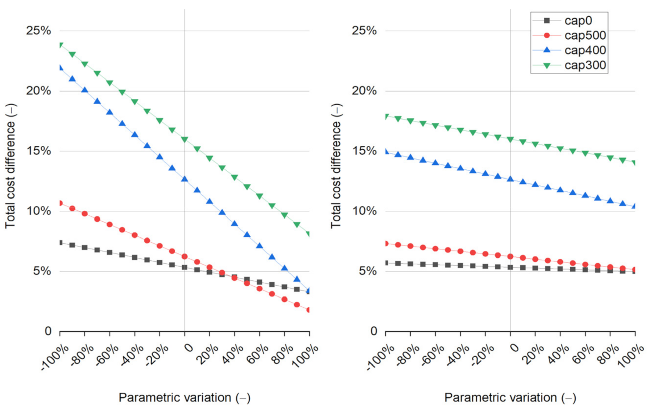
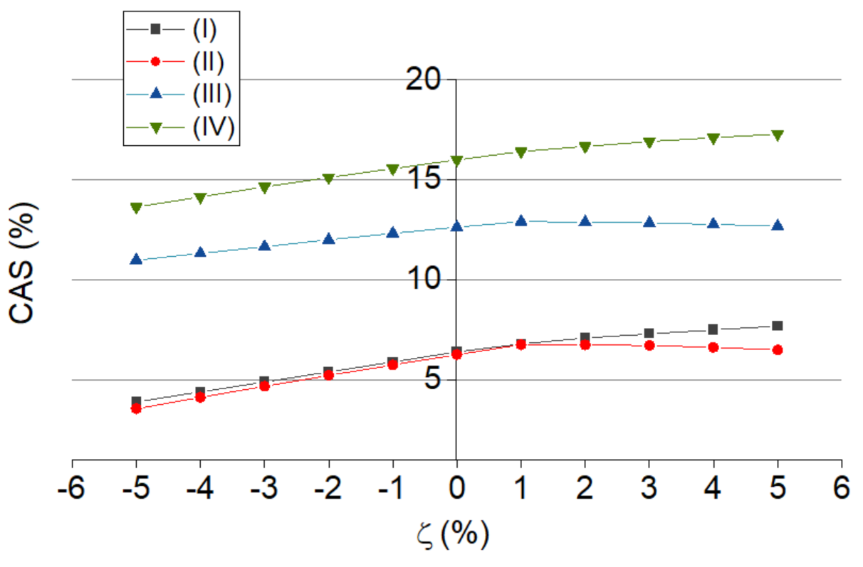
| (I) | DOU = 9; n = 7; no emissions cap |
| (II) | DOU = 2; n = 7; emissions cap: 500 kg/(a*person) |
| (III) | DOU = 1; n = 16; emissions cap: 400 kg/(a*person) |
| (IV) | DOU = 1; n = 15; emissions cap: 300 kg/(a*person) |
Publisher’s Note: MDPI stays neutral with regard to jurisdictional claims in published maps and institutional affiliations. |
© 2021 by the authors. Licensee MDPI, Basel, Switzerland. This article is an open access article distributed under the terms and conditions of the Creative Commons Attribution (CC BY) license (https://creativecommons.org/licenses/by/4.0/).
Share and Cite
Bahret, C.; Eltrop, L. Cost-Optimized Heat and Power Supply for Residential Buildings: The Cost-Reducing Effect of Forming Smart Energy Neighborhoods. Energies 2021, 14, 5093. https://doi.org/10.3390/en14165093
Bahret C, Eltrop L. Cost-Optimized Heat and Power Supply for Residential Buildings: The Cost-Reducing Effect of Forming Smart Energy Neighborhoods. Energies. 2021; 14(16):5093. https://doi.org/10.3390/en14165093
Chicago/Turabian StyleBahret, Christoph, and Ludger Eltrop. 2021. "Cost-Optimized Heat and Power Supply for Residential Buildings: The Cost-Reducing Effect of Forming Smart Energy Neighborhoods" Energies 14, no. 16: 5093. https://doi.org/10.3390/en14165093