Decentralized Optimal Control for Photovoltaic Systems Using Prediction in the Distribution Systems

Abstract

The high penetration of photovoltaic (PV) systems and fast communications networks increase the potential for PV inverters to support the stability and performance of microgrids. PV inverters in the distribution network can work cooperatively and follow centralized and decentralized control commands to optimize energy production while meeting grid code requirements. However, there are older autonomous inverters that have already been installed and will operate in the same network as smart controllable ones. This paper proposes a decentralized optimal control (DOC) that performs multi-objective optimization for a group of PV inverters in a network of existing residential loads and autonomous inverters. The interaction of independent DOC groups in the same network is considered. The limit of PV inverter power factor is included in the control. The DOC is done by the power flow calculation and an autoregression prediction model for estimating maximum power point and loads. Overvoltage caused by prediction errors resulting in non-optimal commands from the DOC is avoided by switching to autonomous droop control (ADC). The DOC and ADC operate at different time scales to take account of communication delays between PV inverters and decentralized controller. The simulation of different scenarios of network control has proved the effectiveness of the control strategies.

1. Introduction

Integrating photovoltaic (PV) energy into the low-voltage distribution system increases network voltage stability issues. With the help of fast communication and smart meters, the smart grid and microgrid can solve distribution network problems through centralized and decentralized controls [1,2]. The increased number of PV systems installed in residential areas can cause reverse power flow when the solar power is higher than the load power. The reverse power flow to the grid causes the voltage in the bus to rise and this is one of the main reasons for the curtailment of PV production [3]. The voltage values in the network should be kept within the statutory limit of 10% higher than the rated value [4]. To reduce the voltage, PV inverters can support a certain amount of reactive power and curtailment of active power through droop control [5,6,7,8,9,10]. Other research studies use optimization methods to avoid overvoltage by calculating the optimal reactive power of PV inverters [11,12]. There are papers applying multi-objective optimal algorithms for obtaining the maximum active power generation and reactive power consumption of the PV inverter with overvoltage control [13,14,15,16]. These control strategies consider the amount of PV reactive power from zero up to the inverter power capacity where the power factor of the PV inverters can be from 0 to 1. However, many conventional PV inverters have a smaller adjustable range, such as from 0.8 to 1 [17,18,19,20]. Therefore, the amount of reactive power from the PV inverters is smaller than those PV inverters with a power factor range of 0 to 1. This leads to more curtailment of PV active power in the case of overvoltage.

A requirement when considering control methods for the smart grid and microgrid is that sufficient information is available for all devices in the network. The optimization controls in [11,12,13,14,15,16] show the results of a network where all PV inverters are controllable. However, in a hybrid network with PV inverters running autonomously and smart PV inverters under central control, the optimization algorithms of the central network controller as in [11,12,13,14,15,16] cannot be performed.

The time to compute an optimal solution for the decentralized controller and the dynamic of the network must also be considered. The state of a network changes every second due to changing solar irradiation and variable residential loads connected to the network. However, there are time lags in the communication between the devices in the network and the central controller and in computing an optimal operating point. Depending on the complexity of the optimization algorithm and the processing power of the computer, the controller may take longer than a second to find an optimal solution. Thus, the time for the controller to give optimal commands to the PV inverters may be longer than the time in which the network changes state.

The state of a network is predicted for the optimization calculation. Previous research forecast the solar profile [21,22,23] for a period of hours or days ahead or for load and solar profiles in the short term, of 15 min [24,25]. In this paper, a simple prediction method is applied for 1 min ahead based on a historical database of 1 h. For a short time prediction, of 1 min, the method has shown its effectiveness in predicting solar and load profiles for the optimization control.

Microgrid communication delay is one of the key challenges to achieving optimal control. The researchers in [26] proposed a maximal delay margin to mitigate the effect of communication delays. In this paper, a different time scale of the PV inverter operation time and the controller computing period is proposed to address the effect of a communication delay.

There is previous research on both the optimization and prediction of PV inverters in microgrids [27,28,29]. However, these research works focused on the optimization of active power production and cost. The investigation of combined optimization with prediction and overvoltage with PV reactive power support is less considered. In the proposed control method, the PV inverters control both active and reactive power by applying multi-objective optimization and prediction.

The prediction may be incorrect due to the uncertainty and stochastic behavior of the load profile or solar irradiation. A vulnerability assessment method for interruptible load employing weights of vulnerability indexes has been proposed [30]. In this paper, a simple method using a voltage gap and delay filter is applied to cope with a quick state change and prediction error.

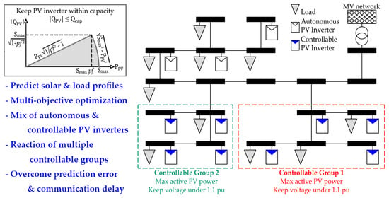
The paper proposes a comprehensive optimal control of smart PV inverters in cluster microgrids in a non-ideal condition of incomplete information and communication delay. The stability and robustness of the proposed control algorithm are proved in different scenarios of both controllable PV inverters and a mix of autonomous and controllable PV inverters.

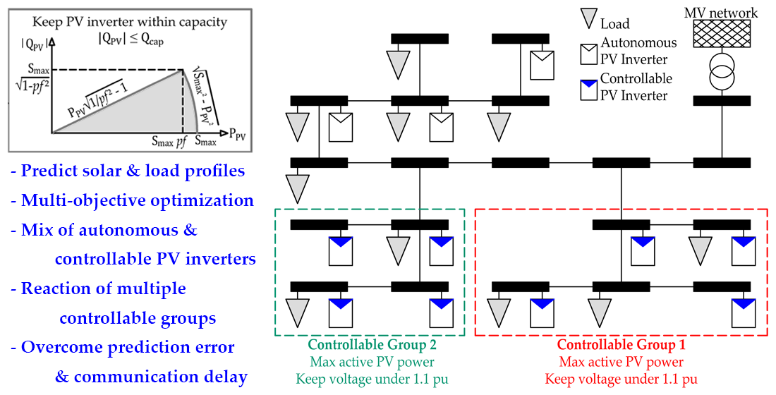
In this paper, an autonomous droop control (ADC) and decentralized optimal control (DOC) are designed for the PV inverters to solve all the problems outlined above. Both control algorithms are designed to always keep the network voltage under the specified value. The limited adjustable range of PV power factor is also taken into account in the control strategies. Based on the voltage, each PV inverter is switched between the ADC and DOC control modes. The DOC can be applied to different independent groups of controllable PV inverters inside a distribution network with a mix of both autonomous and controllable PV inverters. The network interaction of multiple DOC groups is also considered in this study. Moreover, the ADC and DOC control strategies perform their control in different time scales to account for communication and computation time delay while ensuring effective voltage management.

The simulation of the network has been built for verification purposes. The simulation was designed to replicate a practical system with a benchmarked network and a measured solar profile.

2. Inverter Control Strategies

In the low voltage system considered in this work, the control strategies for PV inverters on the network are a mix of those operating autonomously without any outside control and for PV inverters receiving signals from the decentralized control. Autonomous PV inverters without external control operate based solely on the condition of their points of connection and using the ADC as in Figure 1. The PV inverters following the external signals as in Figure 2a, operate in cooperation with other inverters through the DOC in Figure 2b while maintaining the local safety criteria of the grid.

The strategies in Figure 1 and Figure 2 of autonomous and decentralized controls will be discussed in detail in the following sections. In general, all these controls have the two common goals of maintaining the bus voltage under 1.1 pu and keeping the PV inverter operation within their power factor range and power capacity.

2.1. Autonomous Droop Control (ADC)

The flowchart of the ADC is described in Figure 1. The flowchart consists of three main blocks of droop control (block 2), inverter capacity (block 3) and delay filter (block 4). The PV inverters are designed to generate a limited power of ${\mathrm{S}}_{\max }$.

The droop control [5] is designed to keep the voltage under a limit of 1.1 pu. The voltage is regulated by controlling the output reactive and active power of the inverter. The most efficient approach is to use reactive power for voltage support. Therefore, when the voltage is higher than 1.02 pu, the consumption of reactive power ${\mathrm{Q}}_{\mathrm{PV}}$ is linearly increased with increasing voltage. With this reactive power support, the PV inverter can generate active power to the maximum of ${\mathrm{S}}_{\max }$ while the voltage is lower than 1.09 pu. When the voltage exceeds 1.09 pu, overvoltage can be avoided by limiting the active power, which is reduced in inverse proportion to the voltage, as seen in block 2 of Figure 1. The active power output of the PV inverter depends on the maximum power point (MPP) of solar irradiation so that the PV active power ${\mathrm{P}}_{\mathrm{PV}}$ is kept under the droop power limit ${\mathrm{P}}_{\mathrm{droop}}$ or ${\mathrm{P}}_{\mathrm{PV}}\le {\mathrm{P}}_{\mathrm{droop}}$.

After the droop control, the control flow will come to the block of inverter capacity. The relation of the active and reactive power of the PV inverter is shown in block 3 of Figure 1. Depending on the manufacturer’s specification, PV inverters may have an adjustable power factor ranging from $p{f}_{\mathrm{PV}\_\min }$ to 1 so that the inverters can deliver or receive a certain amount of reactive power.

The reactive power ${\mathrm{Q}}_{\mathrm{PV}}$ of the inverter is limited by the lowest power factor value $p{f}_{\mathrm{PV}\_\min }$ and the highest power capacity (${\mathrm{S}}_{\max }$). The absolute value of ${\mathrm{Q}}_{\mathrm{PV}}$ should be less than the maximum amount of reactive power (${\mathrm{Q}}_{\mathrm{cap}}$). The value of ${\mathrm{Q}}_{\mathrm{cap}}$ in block 3 can also be expressed as in Equation (1):

$${\mathrm{Q}}_{\mathrm{cap}}=\{\begin{array}{cc}{\mathrm{P}}_{\mathrm{PV}}\sqrt{\frac{1}{p{f}_{\mathrm{PV}\_\min }^2}-1}& \mathrm{when} {\mathrm{P}}_{\mathrm{PV}}\le {\mathrm{S}}_{\max }p{f}_{\mathrm{PV}\_\min }\\ \sqrt{{\mathrm{S}}_{\max }^2-{\mathrm{P}}_{\mathrm{PV}}^2}& \mathrm{when} {\mathrm{P}}_{\mathrm{PV}}>{\mathrm{S}}_{\max }p{f}_{\mathrm{PV}\_\min }\end{array}$$

(1)

Having computed the ADC setpoints, the system must now avoid controller hunting where the system repeatedly overcorrects itself in one direction and then overcorrects itself in the opposite direction. Hunting in the droop control results from the inverter power decreasing at high voltage, causing the voltage to drop, resulting in the inverter power increasing as the reduced voltage is within limits.

To avoid this effect, a first-order system H(s) is applied [10] with the chosen time constant of 20 s, as seen in block 4 of Figure 1. By doing this, the control signal is applied gradually to the inverter and the hunting effect is avoided. The function H(s) is the continuous-time transfer function; to be able to use it in the simulation, H(s) should be changed to the discrete-time function H(z) through the MATLAB c2d function [31] with a sample time of Ts second(s).

2.2. Smart Inverter Control (SIC)

The SIC is applied for controllable inverters that can both operate autonomously and follow a decentralized controller. The SIC is a mechanism of switching smart PV inverters between the ADC and the DOC modes. Similar to the ADC in Figure 1, the SIC in Figure 2a follows the same steps of the droop control (block 3a), inverter capacity (block 5a) and first-order system (block 6a). The only difference is that the inverter will operate under the command of the DOC when the measured voltage is less than or equal to 1.098 pu, as seen in blocks 2a and 4a. This means that the smart PV inverter mainly functions under the instructions of the DOC and operates with ADC only when the voltage is close to the upper limit. The ADC is integrated into the smart inverter to ensure that in the case that there is any faulty command from the DOC, the system would still be stable. The DOC is described in the following section.

3. Decentralized Optimal Control (DOC)

The DOC in Figure 2b is the control algorithm that sends commands to a group of smart PV inverters in a certain area. This control calculates both active and reactive power of PV inverters so all inverters work cooperatively to meet all safety requirements with optimum performance. To do this, a power flow analysis is applied to calculate the network voltage for a range of possible PV output power values. Therefore, knowing the network state, such as power absorbed or delivered to the controllable area, is one of the initial steps.

There are not only PV inverters but also existing loads in the network. Knowledge of the power of all components is necessary for power flow analysis. Hence, measurement of all components such as power and voltage values should be collected for the DOC. Moreover, the time lag resulting from communication delays and the large number of calculations required to determine the DOC setpoints limits the operational frequency of the central controller. In this work, the commands from the DOC are sent to PV inverters every minute.

To determine the setpoint values for PV inverters in the next minute, the control should estimate the state of the network in that next minute by a prediction method. As seen in blocks 2b and 3b of Figure 2b, the prediction is done before the power flow analysis in block 4b. More details of the prediction mechanism are described in Section 3.1.

In block 4b, the Newton-Raphson power flow method [32] is applied to calculate the voltage of PV buses in the next minute based on the predicted values in block 3b. The state of the network is considered in the worst-case scenario of maximum PV active power (${\mathrm{P}}_{\mathrm{PV}}={\mathrm{P}}_{\mathrm{MPP}\_\mathrm{predicted}}$) and zero reactive power (${\mathrm{Q}}_{\mathrm{PV}}=0$). The reactive power from the PV inverters can affect the inverter lifetime and cost [33] so that a zero reactive power is applied.

To save unnecessary calculation, after the power flow analysis, the optimization is only performed when any node voltage exceeds 1.095 pu, as shown in block 5b. When all predicted voltage values are under 1.095 pu, the DOC only commands the PV inverters to run the MPP with the unity power factor, as seen in block 7b.

The optimization in block 6b is updated every minute and it is used to maximize the active power of all PV inverters in the controllable group while keeping the inverters within limits of the power factor ($p{f}_{\mathrm{PV}\_\min }$) and power capacity (${\mathrm{S}}_{\max }$).

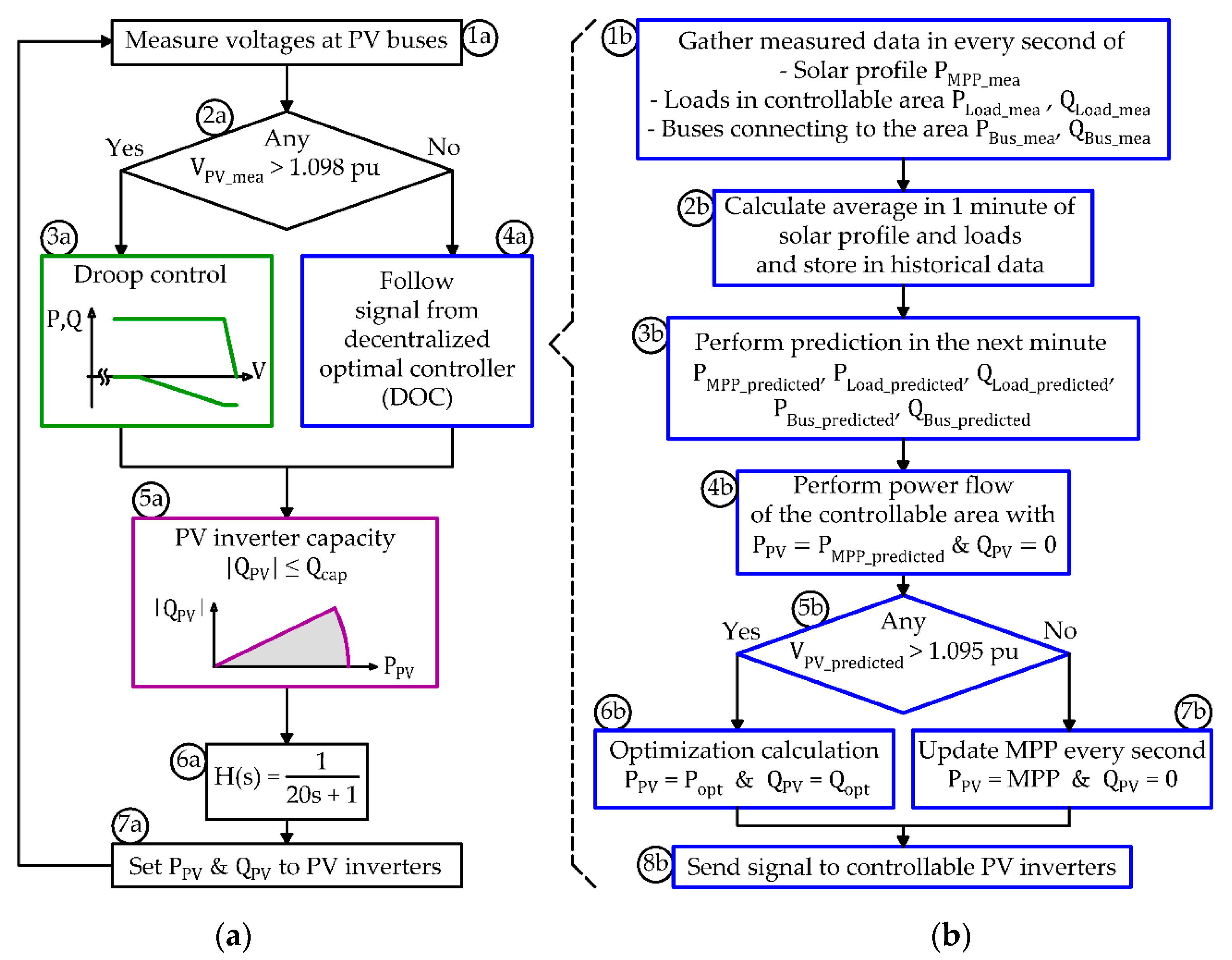
The different control time scales are illustrated in Figure 3. In this figure, a section of 180 s or 3 min is shown. In Figure 3a, the ADC is updated every second, i.e., it is running 180 times within 3 min.

The illustration of blocks 5b, 6b and 7b of Figure 2b is shown in Figure 3b,c. When all predicted voltage values are under 1.095 pu, the DOC just commands the PV inverters to run the MPP every second. When the predicted voltage is higher than 1.095 pu, the optimization is applied. The optimization is calculated and the DOC command remains unchanged for every minute. As seen in Figure 3b, the predicted power flow voltage shows that the voltage value will be higher than 1.095 pu in the second and third minutes, and thus, optimization (block 6b) is applied during these two minutes.

The prediction model can output inaccurate values due to many factors, such as a sudden change of solar irradiation, random behavior of the load profile, network problems or missing communication. A low level of prediction error is acceptable as the control algorithm includes a voltage gap between 1.095 pu to 1.098 pu for small fluctuations of the solar or load profile. However, when the measured voltage is over the threshold of 1.098 pu (block 2a of Figure 2a), the DOC commands to the PV inverters must be overridden and the PV inverters switch to the failsafe autonomous mode of ADC. The illustration of SIC when there are prediction inaccuracies is shown in Figure 3d,e. In this situation, the measured PV voltage ${\mathrm{V}}_{\mathrm{PV}\_\mathrm{mea}}$ is larger than 1.098 pu at the first and third minutes. The ADC will override the DOC from the time of the interruption until the next minute. This is to avoid the hunting effect of switching back and forth between the ADC and the DOC. As seen in Figure 3e, the PV inverter switches to ADC mode when the measured voltage is larger than 1.098 pu and it keeps running the ADC until the end of a minute.

The description detailing the mechanism of the prediction calculation and optimization is presented in Section 3.1 and Section 3.2.

3.1. Prediction

There are many typical time series forecasting methods, such as Autoregression (AR), Moving Average (MA), Autoregressive Moving Average (ARMA), Autoregressive Integrated Moving Average (ARIMA), Regression Model with ARIMA Error, Vector Autoregression (VAR), Generalized Autoregressive Conditionally Heteroscedastic model (GARCH), Seasonal Autoregressive Integrated Moving-Average (SARIMA) and Seasonal Autoregressive Integrated Moving Average with Exogenous Regressors (SARIMAX) [34]. These methods can be applied to predict more than one point ahead. In this paper, one point ahead is sufficient for the next step of the optimization calculation. Therefore, the AR forecasting method was chosen for its simplicity.

The AR model calculates the predicted value ${\mathrm{y}}_{{\mathrm{T}}^{*}}$ based on previous values. The $\mathrm{p}$^th-order autoregression model, written as AR($p$), is a multiple linear regression where the predicted value of the series ${\mathrm{y}}_{{\mathrm{T}}^{*}}$ is a function of ${\mathrm{y}}_{\mathrm{T}-1}$, ${\mathrm{y}}_{\mathrm{T}-2}$, …, ${\mathrm{y}}_{\mathrm{T}-\mathrm{p}}$. In this research, the MATLAB arcov function [35] is used to fit an AR($\mathrm{p}$) model to the input signal by the covariance method. 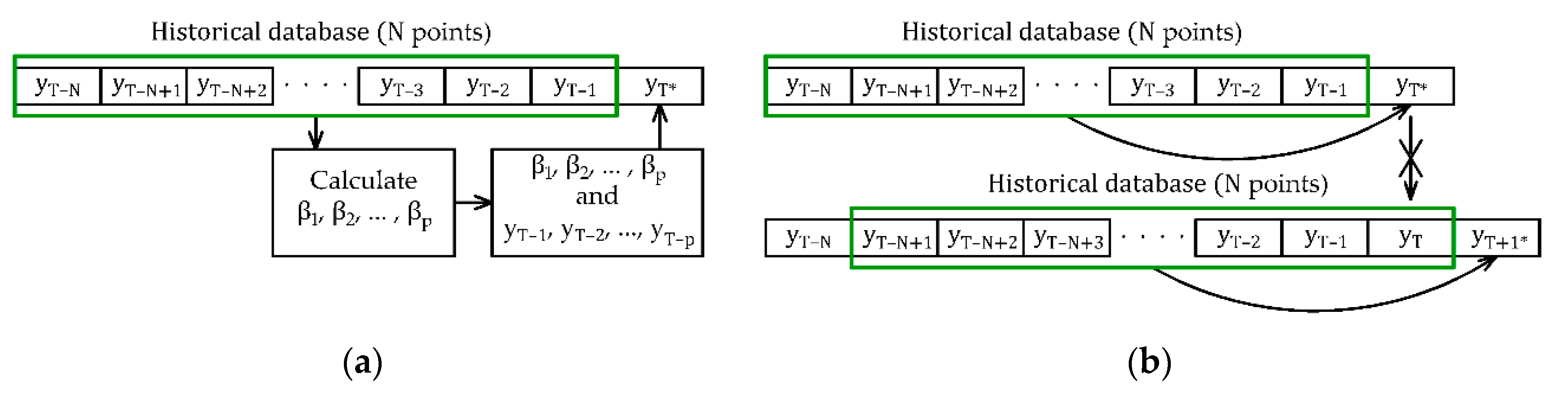This function calculates coefficients ${\mathsf{\beta }}_1$, ${\mathsf{\beta }}_2$, …, ${\mathsf{\beta }}_{\mathrm{p}}$ from the input signal of $\mathrm{N}$ points ${\mathrm{y}}_{\mathrm{T}-1}$, ${\mathrm{y}}_{\mathrm{T}-2}$, …, ${\mathrm{y}}_{\mathrm{T}-\mathrm{N}}$, as seen in Figure 4a.

The predicted value ${\mathrm{y}}_{{\mathrm{T}}^{*}}$ is calculated from previous values ${\mathrm{y}}_{\mathrm{T}-1}$, ${\mathrm{y}}_{\mathrm{T}-2}$, …, ${\mathrm{y}}_{\mathrm{T}-\mathrm{p}}$ and calculated coefficients ${\mathsf{\beta }}_1$, ${\mathsf{\beta }}_2$, …, ${\mathsf{\beta }}_{\mathrm{p}}$, as in Equation (2). It is noted in Equation (2) that the predicted value ${\mathrm{y}}_{{\mathrm{T}}^{*}}$ is determined only from $\mathrm{p}$ values of ${\mathrm{y}}_{\mathrm{T}-1}$, ${\mathrm{y}}_{\mathrm{T}-2}$, …, ${\mathrm{y}}_{\mathrm{T}-\mathrm{p}}$, but the coefficients ${\mathsf{\beta }}_1$, ${\mathsf{\beta }}_2$, …, ${\mathsf{\beta }}_{\mathrm{p}}$ are calculated from $\mathrm{N}$ values of ${\mathrm{y}}_{\mathrm{T}-1}$, ${\mathrm{y}}_{\mathrm{T}-2}$, …, ${\mathrm{y}}_{\mathrm{T}-\mathrm{N}}$. The larger the value of $\mathrm{N}$, the more accurate the values of coefficients ${\mathsf{\beta }}_1$, ${\mathsf{\beta }}_2$, …, ${\mathsf{\beta }}_{\mathrm{p}}$.

$${\mathrm{y}}_{{\mathrm{T}}^{*}}={\mathsf{\beta }}_1{\mathrm{y}}_{\mathrm{T}-1}+{\mathsf{\beta }}_2{\mathrm{y}}_{\mathrm{T}-2}+\dots +{\mathsf{\beta }}_{\mathrm{p}}{\mathrm{y}}_{\mathrm{T}-\mathrm{p}}$$

(2)

The prediction value may be incorrect or too far away from the real value so that there is a limit to the predicted value ${\mathrm{y}}_{{\mathrm{T}}^{*}}$ to be in the range of ±50% and has the same sign as the previously measured value ${\mathrm{y}}_{\mathrm{T}-1}$. When the predicted value is outside the range or has the opposite sign, it will be set to be the same as the previously measured value as in Equation (3):

$$\mathrm{If}\left|{\mathrm{y}}_{{\mathrm{T}}^{*}}\right|>1.5\left|{\mathrm{y}}_{\mathrm{T}-1}\right|\mathrm{or}\left|{\mathrm{y}}_{{\mathrm{T}}^{*}}\right|<0.5\left|{\mathrm{y}}_{\mathrm{T}-1}\right|\mathrm{or}{\mathrm{y}}_{{\mathrm{T}}^{*}}\times {\mathrm{y}}_{\mathrm{T}-1}<0\mathrm{then}{\mathrm{y}}_{{\mathrm{T}}^{*}}={\mathrm{y}}_{\mathrm{T}-1}$$

(3)

The historical database for the prediction is a fixed $\mathrm{N}$ point, and the database is updated before any new prediction, as seen in Figure 4b. In addition, all $\mathrm{N}$ values stored in the database are measured values from which the predicted point (only one point) is always calculated. As seen in Figure 4b, the predicted value ${\mathrm{y}}_{{\mathrm{T}}^{*}}$ is not included in the database of the next prediction. The database is updated with the addition of the measured or actual value of ${\mathrm{y}}_{\mathrm{T}}$ and the removal of ${\mathrm{y}}_{\mathrm{T}-\mathrm{N}}$. Additionally, the coefficients of ${\mathsf{\beta }}_1$, ${\mathsf{\beta }}_2$, …, ${\mathsf{\beta }}_{\mathrm{p}}$ are updated from the new database for the next prediction.

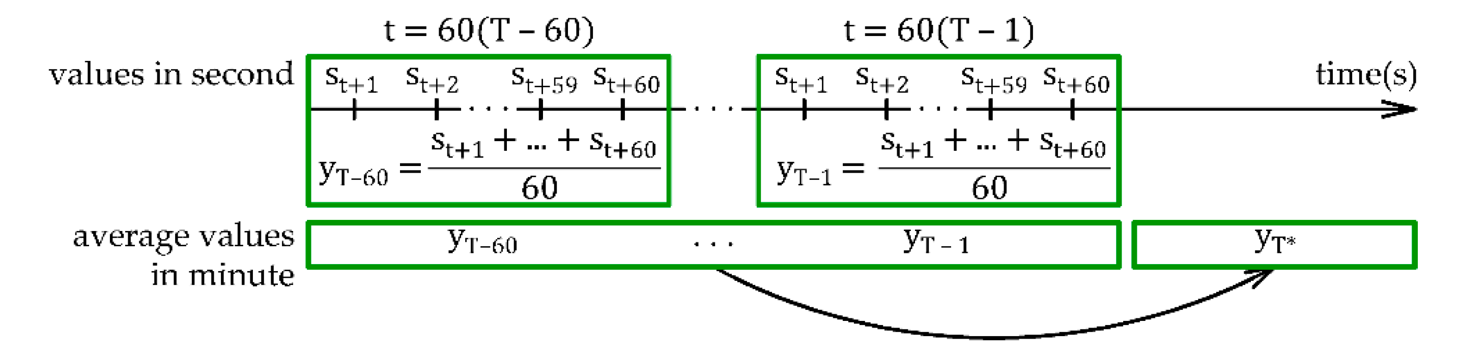
In this paper, the third-order autoregression, or AR(3), is selected. A database section of 60 points is chosen ($\mathrm{N}=60$). As seen in Equation (2), the predicted value ${\mathrm{y}}_{{\mathrm{T}}^{*}}$ is determined from three previous values of ${\mathrm{y}}_{\mathrm{T}-1}$, ${\mathrm{y}}_{\mathrm{T}-2}$ and ${\mathrm{y}}_{\mathrm{T}-3}$. The three coefficients ${\mathsf{\beta }}_1$, ${\mathsf{\beta }}_2$ and ${\mathsf{\beta }}_3$ are calculated from 60 values of ${\mathrm{y}}_{\mathrm{T}-1}$, …, ${\mathrm{y}}_{\mathrm{T}-60}$. In this paper, the new data are updated every minute and taken from an average of 60 s, as shown in Figure 5.

Figure 5 illustrates the mechanism of the first three blocks in Figure 2b (blocks 1b, 2b and 3b). Network values are measured every second as ${\mathrm{s}}_{\mathrm{t}+1}$, ${\mathrm{s}}_{\mathrm{t}+2}$, …, ${\mathrm{s}}_{\mathrm{t}+60}$ over one minute (block 1b); then, the value of every minute (${\mathrm{y}}_{\mathrm{T}-1}$, …, ${\mathrm{y}}_{\mathrm{T}-60}$) is calculated by taking the average of 60 one-second measured values (block 2b). After that, the value in the next minute ${\mathrm{y}}_{{\mathrm{T}}^{*}}$ is calculated from the 60 average minute values (${\mathrm{y}}_{\mathrm{T}-1}$, …, ${\mathrm{y}}_{\mathrm{T}-60}$). This means that the predicted values are calculated from data of 3600 s or 1 h.

The next step of the smart inverter control is the optimization calculation.

3.2. Optimization

The calculation burden for the DOC is reduced by only applying the optimization process when the maximum voltage calculated from the power flow analysis is higher than 1.095 pu, as seen in blocks 5b and 6b of Figure 2b. To calculate the multi-objective optimization, the MATLAB function fmincon [36] is used. This function determines optimal values of a cost function with boundaries, equality, linear inequality and non-linear inequality constraints and is, therefore, suitable for this research.

The goal of the optimization is to maximize the active power of $n_{\mathrm{PV}}$ inverters while keeping all node voltages under 1.095 pu. The PV inverters can consume a certain amount of reactive power (${\mathrm{Q}}_{\mathrm{PV}}\le 0$) to help reduce the bus voltage if required. The objective function is shown in Equation (4). The power ${\mathrm{P}}_{\mathrm{PV}}$ and ${\mathrm{Q}}_{\mathrm{PV}}$ are the variables to be determined by the optimization so that there are a total of 2$n_{\mathrm{PV}}$ variables:

$$\mathrm{Objective}=\min \left(-{{\displaystyle \sum }}_{i=1}^{n\mathrm{P}\mathrm{V}}{\mathrm{P}}_{\mathrm{PV}\left(i\right)}+{{\displaystyle \sum }}_{i=1}^{n\mathrm{P}\mathrm{V}}{\mathrm{Q}}_{\mathrm{PV}\left(i\right)}\right)$$

(4)

Any PV inverter $i$ has its upper and lower boundaries for active and reactive power, shown in Equations (5) and (6), respectively. Active power delivered from the PV inverter is positive and limited to the power available at the MPP, while the reactive power consumed by the inverter is negative. Note that the MPP used in the optimization is the predicted value. The lower limit of ${\mathrm{Q}}_{\mathrm{PV}}$ also depends on the MPP and has one of two possible values. These values relate to the linear and non-linear operating regions when ${\mathrm{P}}_{\mathrm{MPP}}$ is less or greater than ${\mathrm{S}}_{\max }p{f}_{\mathrm{PV}\_\min }$, as in Equation (6). In the non-linear region, the lower limit of ${\mathrm{Q}}_{\mathrm{PV}}$ is set to be fixed and does not depend on ${\mathrm{P}}_{\mathrm{MPP}}$:

$$0\le {\mathrm{P}}_{\mathrm{PV}\left(i\right)}\le {\mathrm{P}}_{\mathrm{MPP}\left(i\right)}$$

(5)

$$\begin{array}{cc}-{\mathrm{P}}_{\mathrm{MPP}\left(i\right)}\sqrt{\frac{1}{p{f}_{\mathrm{PV}\_\min \left(i\right)}^2}-1}& {\mathrm{when}\mathrm{P}}_{\mathrm{MPP}\left(i\right)}\le {\mathrm{S}}_{\max \left(i\right)}p{f}_{\mathrm{PV}\_\min \left(i\right)}\\ -{\mathrm{S}}_{\max \left(i\right)}\sqrt{1-p{f}_{\mathrm{PV}\_\min \left(i\right)}^2}& \mathrm{when} {\mathrm{P}}_{\mathrm{MPP}\left(i\right)}>{\mathrm{S}}_{\max \left(i\right)}p{f}_{\mathrm{PV}\_\min \left(i\right)}\end{array}\}\le {\mathrm{Q}}_{\mathrm{PV}\left(i\right)}\le 0$$

(6)

Ensuring that the power factor of each PV inverter is within the limit introduces the linear inequality constraint shown in Equation (7). The value of ${\mathrm{Q}}_{\mathrm{PV}}$ is set to be within the power factor constraint of the PV inverter relative to ${\mathrm{P}}_{\mathrm{PV}}$:

$${\mathrm{Q}}_{\mathrm{PV}\left(i\right)}\ge -{\mathrm{P}}_{\mathrm{PV}\left(i\right)}\sqrt{\frac{1}{p{f}_{\mathrm{PV}\_\min \left(i\right)}^2}-1}$$

(7)

Nonlinear inequality constraints are shown in Equations (8) and (9). The voltage at all nodes in Equation (8) is a function of ${\mathrm{P}}_{\mathrm{PV}}$ and ${\mathrm{Q}}_{\mathrm{PV}}$. The voltage value is calculated through the Newton-Raphson power flow method [32] and must remain within network limits. The voltage limit is chosen to be 1.095 pu, the same as the value in block 5b of Figure 2b. The inverter capacity is limited by Equation (9):

$$\left|{\mathrm{V}}_{\mathrm{PV}\left(i\right)}\right|\le 1.095$$

(8)

$${\mathrm{Q}}_{\mathrm{PV}\left(i\right)}^2+{\mathrm{P}}_{\mathrm{PV}\left(i\right)}^2\le {\mathrm{S}}_{\max \left(i\right)}^2$$

(9)

The starting points of the active and reactive power variables are shown in Equation (10). The active power equals the maximum possible MPP values; the reactive power starts from zero:

$${\mathrm{P}}_{\mathrm{PV}\left(i\right)}^{\left(0\right)}={\mathrm{P}}_{\mathrm{MPP}\left(i\right)}\mathrm{and}{\mathrm{Q}}_{\mathrm{PV}\left(i\right)}^{\left(0\right)}=0$$

(10)

The reason for setting the voltage limit to 1.095 pu instead of 1.1 pu is that the optimization calculation is based on the predicted values and the results may be incorrect. There is a range from 1.098 to 1.1 pu in which the inverter power is limited by the droop control. In this way, if there is any decentralized controller prediction or calculation error, the voltage is always kept under the upper limit.

The control theories presented above are coded in the simulation environment to assess the potential of the different control strategies.

4. Simulation

4.1. System Confirguration

The simulation in this research is based on the benchmark of a 20-bus 400 V line-to-line network [37], as shown in Figure 6. The 20 buses are labeled from C1 to C20, where bus C1 is the swing bus, whose voltage is 1.02 pu. In this network, there are three types of distribution lines (OH1–OH3), whose impedance values are shown in Figure 6.

There are 11 PV inverters (PV1–PV11) and 10 loads (Load1-Load10) that are placed in the network. There are two groups of buses with DOC applied. Group 1 contain buses from C10 to C14 with four PV inverters (PV3–PV6) and three loads (Load5–Load7). Buses C15 to C18 are in Group 2 with four PV inverters (PV7–PV10) and two loads (Load8–Load9). These two groups will operate with independent DOCs.

The simulation is conducted in MATLAB/Simulink in phasor mode at a frequency of 50 Hz and a sample time Ts of 1 s over a day of 24 h or 86,400 s.

All 11 PV inverters (PV1–PV11) have the same MPP profile based on measured irradiation [38], as shown in Figure 7a. These PV inverters have the power capacity ${\mathrm{S}}_{\max }$ of 30 kVA and adjustable power factor range from 0.8 to 1 or $p{f}_{\mathrm{PV}\_\min }$ is equal to 0.8. It is noted that the MPP profile has a dropdown spike due to the sudden change of solar irradiation at around 2:32 pm. This spike would cause prediction errors for available PV power and will lead to optimization errors for the DOC controller that will be discussed in the simulation results.

All 10 loads (Load1–Load10) have the same power profile [37], as shown in Figure 7b. Along with active power, these loads are set to consume an amount of reactive power and the power factor of all these loads is chosen to have 0.95 lagging. The power values of the loads are negative, showing that these loads are consuming both active and reactive power.

The DOC for Group 1 is shown in Figure 8a. The power flow analysis is only applied for nine buses (C1–C4 and C10–C14). The power flow through bus C4 is considered a virtual load. The value of this load is the total measured power that flows through its bus. This virtual load is bidirectional, which means it can either consume or generate power. The direction of this load depends on the sum of power flowing through it. The virtual load is simply the power that flows through a bus and is predicted as described in blocks 1b, 2b and 3b of Figure 2b.

The DOC for Group 2 is presented in Figure 8b. The power flows through buses C6 and C10 are measured and communicated back to the DOC as virtual loads.

For Group 1, the prediction is conducted for loads at C11, C12 and C14 and the virtual load at C4. Loads at C15 and C17 and virtual loads at C6 and C10 are predicted for Group 2.

The voltage change of any bus in the 20-bus network affects the others buses’ voltage; therefore, to perform the power flow analysis, power inputs of all devices connecting to 20 buses have to be known. However, there are autonomous PV inverters and existing loads in the network without measurement or communication so that it is impossible for the power flow calculation. In the 20-bus network, there are only five buses in Group 1 and four buses in Group 2. The controller of each group can only access the data of its controllable area so that the optimization or power flow cannot be achieved without the application of virtual load. By applying the concept of virtual load, the DOC does not need to know all the power values in the network and can still proceed with the power flow analysis and optimization calculation.

The simulation is conducted for five cases. In Case 1, all PV inverters are running in autonomous mode using the ADC shown in Figure 1. In Case 2, the PV inverters in Group 1 operate using the DOC as shown in Figure 2a,b, while the other PV inverters use ADC. In Case 3, only Group 2 is controlled by the DOC, while others apply the ADC. In Case 4, Group 1 and Group 2 are running the DOC, but they are operating independently. In Case 5, all PV inverters follow one DOC. A summary of the five simulation cases is presented in

Table 1. Cases applied in the simulation.

Case #	Case Description	Group 1 (PV3–PV6)	Group 2 (PV7–PV10)	Other PVs (PV1, PV2, PV11)
1	ADC for all	ADC	ADC	ADC
2	DOC for Group 1	DOC1	ADC	ADC
3	DOC for Group 2	ADC	DOC2	ADC
4	DOC for Groups 1 and 2	DOC1	DOC2	ADC
5	DOC for all	DOC	DOC	DOC

.

4.2. Results

The network was simulated for each of the five cases in Table 1. In each control case, the voltage, active power, PV inverter power factor and the apparent power are presented.

The results of Case 1, in which all 11 PV inverters are running the ADC, are shown in Figure 9. The voltages of all PV inverters are under 1.1 pu. The voltages at PV1, 2 and 3 are lower than other PVs so that the active power at PV1, 2 and 3 have the complete MPP profile, while the output active power of the other PV systems is curtailed at the peak time to reduce the node voltage. The power factor values of all PV inverters $p{f}_{\mathrm{PV}}$ have a minimum value of 0.8. The reactive power consumption of PV inverters is proportional to the voltage level; in other words, the higher the voltage, the higher the consumption of reactive power. The apparent power, which is the combination of the active and reactive power, is always kept under the limit of 30 kVA.

Figure 10 shows the results of Case 2 when only the four PV inverters in Group 1 (PV3–PV6) are controlled by the DOC. As seen for the connection of Group 1 in Figure 6, PV4 and PV5 at buses C12 and C13 are at the termination of the network. The reverse power flows from PV4 and PV5 cause voltage levels at buses C12 and C13 to be higher than the voltages at buses C10 and C14. Therefore, the active power amount of PV4 and PV5 has the most curtailment in comparison to PV3 and PV6. Moreover, the voltage levels at buses C10 and C14 also affect the voltage levels at buses C12 and C13. Therefore, the active power of PV3 and PV6 is also curtailed to keep the voltage of all four PV buses below the limit. The voltages at buses C12 and C13 reach 1.095 pu and maintain this level at peak time.

The results of the Case 3 optimization of the four PV inverters in Group 2 (PV7–PV10) are presented in Figure 11. Buses C17 and C18 have higher voltages than buses C15 and C16 because of the reverse power flow. Thus, the active power curtailment of PV9 and PV10 is higher than PV7 and PV8. Similar to Case 2, the power factor values of all four PV inverters are at the lowest value of 0.8 to lower the network voltage when there is high irradiation.

Figure 12 shows the results of Case 4 when two DOCs are applied independently for Group 1 (PV3–PV6) and Group 2 (PV7–PV10). Similar to Figure 10 and Figure 11, the voltage, power factor and apparent power are kept within limits.

The results for when all PV inverters follow a DOC (Case 5) are presented in Figure 13. With this control strategy, 11 PV inverters are communicating and working together to achieve a common goal of maintaining the voltages under the limit and optimizing the active power. The active power of all PV inverters are collectively curtailed to improve the total energy yield.

Figure 14 shows a summary of active power output for the five simulated cases. In Figure 14a, the total active power of all PV inverters for each simulation case during a day is plotted. Case 1 to Case 4 have high curtailment at peak time in comparison to Case 5, where all PV inverters work together. The total energy output of all PV inverters in the network is shown in Figure 14b. The ADC yields the lowest energy, while the DOC has the highest value.

In general, all five cases in the simulation show that the voltage values of all PV buses are kept under 1.1 pu as expected. The power factor values of the PV inverters are higher or equal to 0.8. The apparent power is kept within the inverter capacity.

5. Result Summary and Discussion

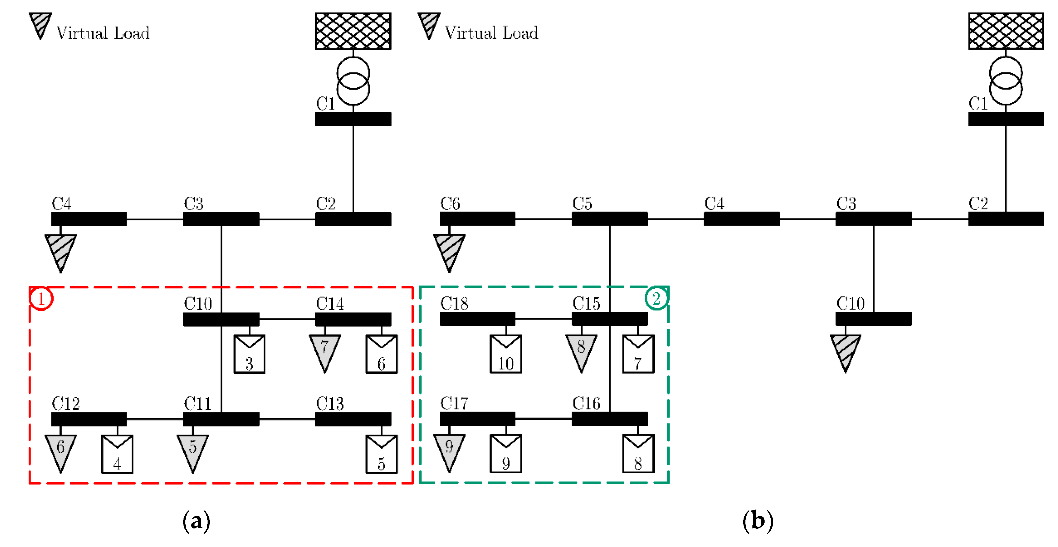
This paper has presented complete control strategies for PV inverters. The network responses with different control groups were realized in the simulation results. The DOC is improved by making the power flow analysis possible for a small area inside a larger network, as seen in Figure 8 by virtual loads and prediction. The switching between the DOC and ADC is also a contribution to robustly keep the network in a stable state even in the event of incorrect commands from the DOC.

The control mechanism of the ADC partially acts as an optimization method. As seen in block 2 of Figure 1, the higher the voltage, the lower the active power and the higher the reactive power. The reverse power flow causes the voltage of PV buses at the termination buses of the network to have the highest value. With the ADC, the power delivered at these buses has the most curtailment, and the reactive power has the most consumption. This leads to higher power production for PV inverters at the other buses in the network. The ADC in this research has shown its effectiveness of voltage limiting without any outer controller. The ADC also considers the power factor limit of each PV inverter.

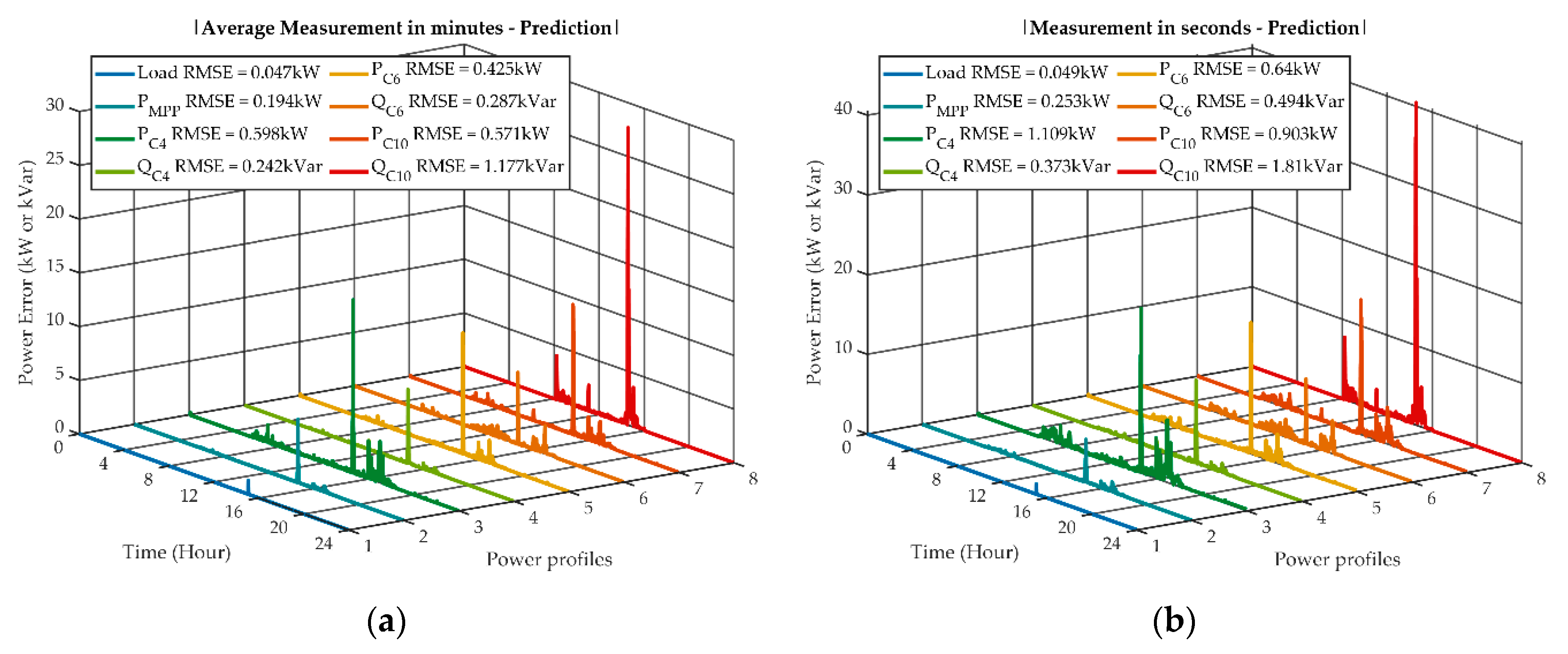
The AR prediction model is one of the key factors to make optimization possible. To calculate the accuracy of the prediction, the root-mean-square error (RMSE) [39] between the actual profile and the prediction is calculated with Equation (11):

$$\mathrm{RMSE}=\sqrt{\frac{1}{T}{{\displaystyle \sum }}_{t=1}^T{\left(y_{\mathrm{actual}\left(t\right)}-y_{\mathrm{predicted}\left(t\right)}\right)}^2}$$

(11)

The RMSE values and absolute errors of the prediction and power profiles of load profile, MPP profile and virtual loads for Case 4 are shown in Figure 15. The reactive power of the load profile has the same shape as the active power shown in Figure 7b, so that only load active power ${\mathrm{P}}_{\mathrm{Load}}$ is shown. For the virtual loads, the prediction is shown for both the active and reactive power.

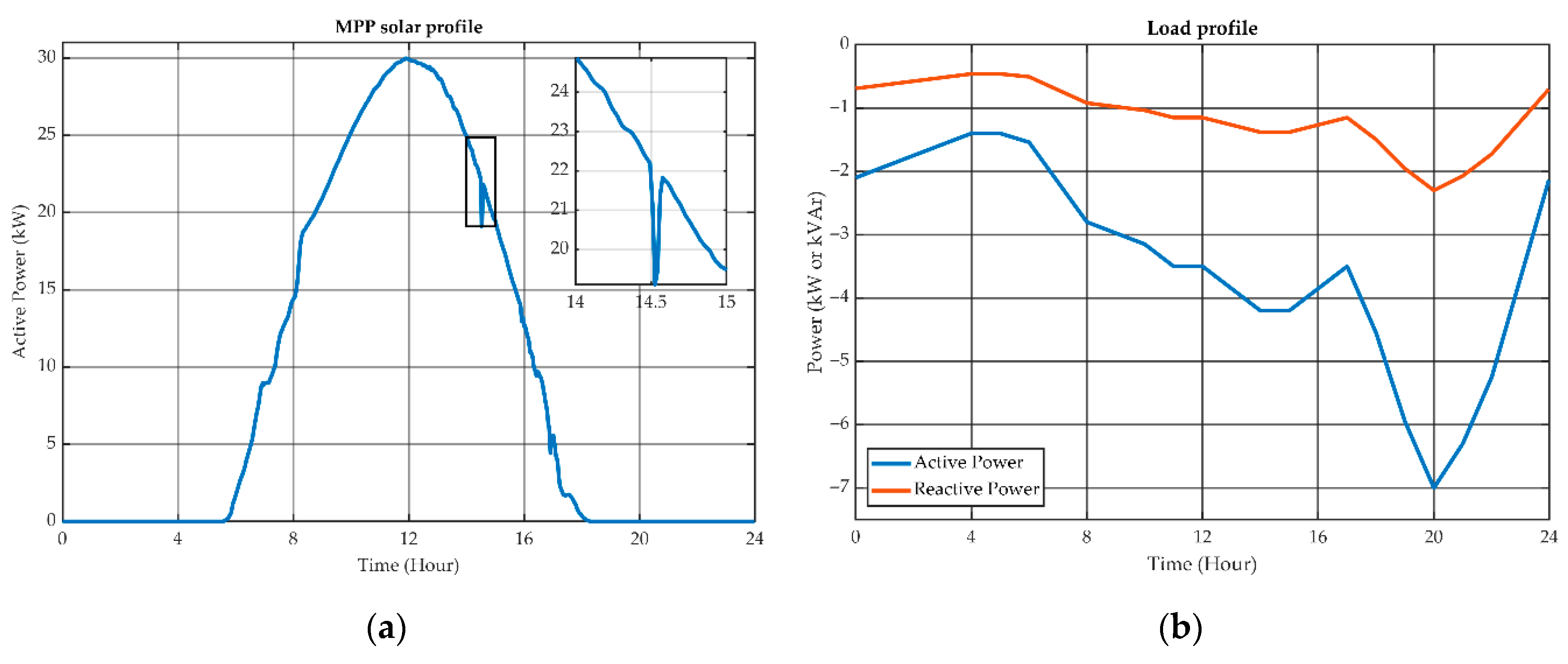
The differences between the prediction and the average values for every minute are shown in Figure 15a. The error for the load and MPP profile is low with a few spikes. As seen in Figure 7a, there is a small drop of solar power at around 2:32 pm, causing an error spike in the prediction. The errors for virtual loads are higher than the load and MPP profile, but the differences are small, with the highest RMSE of 1.177 kVar.

The absolute errors between the actual load profiles in every second and the prediction are shown in Figure 15b. As mention before, the prediction is determined for every minute and shows the tendency of the values in the next 60 s. During a period of 60 s, there are changes in the power values; thus, there are more errors in Figure 15b in comparison to Figure 15a.

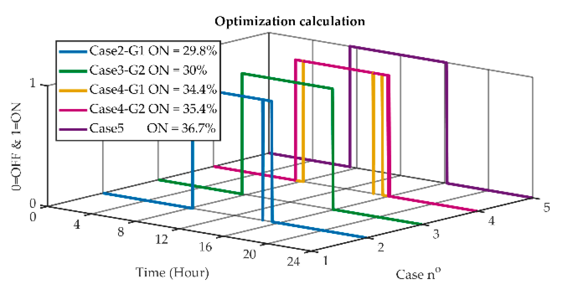
The prediction described in block 3b of Figure 2b operates whenever there is PV power available and the optimization calculation (block 6b of Figure 2b) is only utilized when the predicted power flow voltage is larger than 1.095 pu. The results of the simulation show that the optimization calculation is only applied at peak time when the solar irradiation is high. In the simulation, the optimization operates for about 35% of the time in a day, as seen in Figure 16. The simulation of Case 1 is the ADC so that the optimization is not applied. Case 4 has two DOCs operating separately, so that there are two lines of optimization calculation for Group 1 and Group 2 in Figure 16. The optimal controller does not need to run all the time to reduce the power consumption of the controller.

In Figure 16, the optimization calculation in Case 4 of Group 2 is applied for a longer time than Group 1, because the PV inverters in Group 2 are located further from the swing bus than those in Group 1. The reverse power flow causes the voltage levels in Group 2 to be higher than those in Group 1, so that Group 2 has to operate more calculations than Group 1.

The analysis of Figure 16 indicates that there is a short time at around 2:32 pm when the optimization does not operate (the PV inverters operate as in block 7b of Figure 2b instead), as seen in Case 2 and Group 1 of Case 4. The sudden drop in solar irradiation highlighted in Figure 7a results in PV power prediction errors, leading to the brief override of the optimization algorithm with ADC, as illustrated in Figure 3.

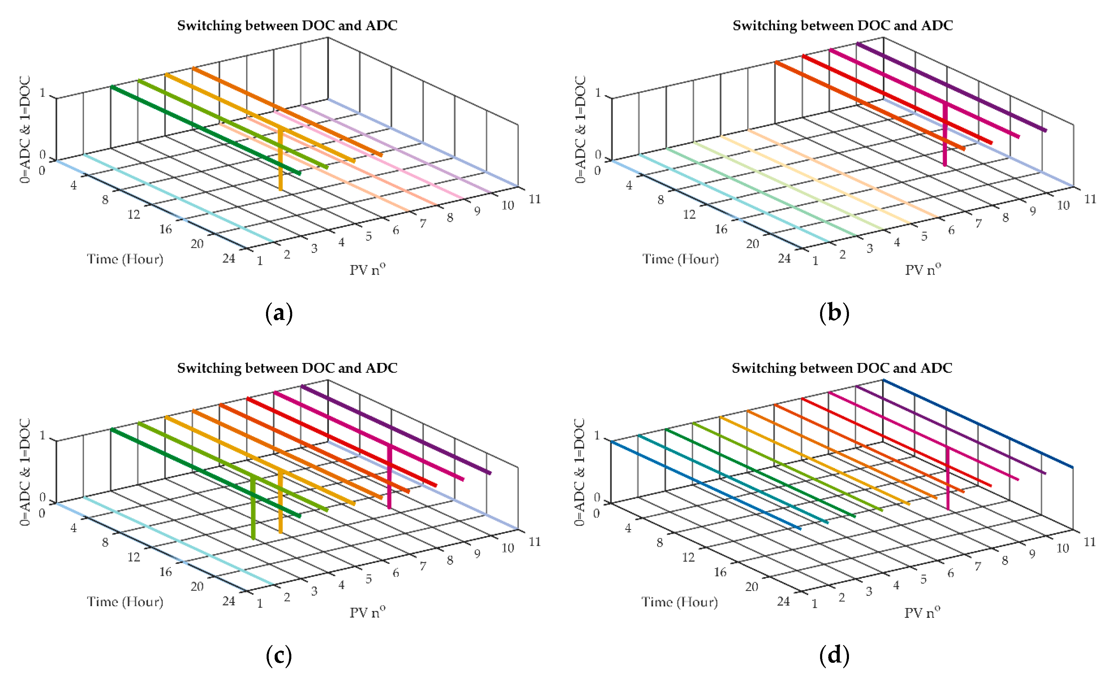
Figure 17 shows the switching between the DOC and ADC when there are prediction errors, causing the voltage to be higher than 1.098 pu as block 2a of Figure 2a. Simulation Case 2 to Case 5 are shown. The controllable PV inverters switch back to the ADC at the time of the prediction error at 2:32 pm. As seen in the figure, not all PV inverters switch back to ADC, even though the prediction error of the solar profile is the same for all inverters. There is an allowable gap from 1.095 pu to 1.098 pu for PV inverters to behave with the prediction errors.

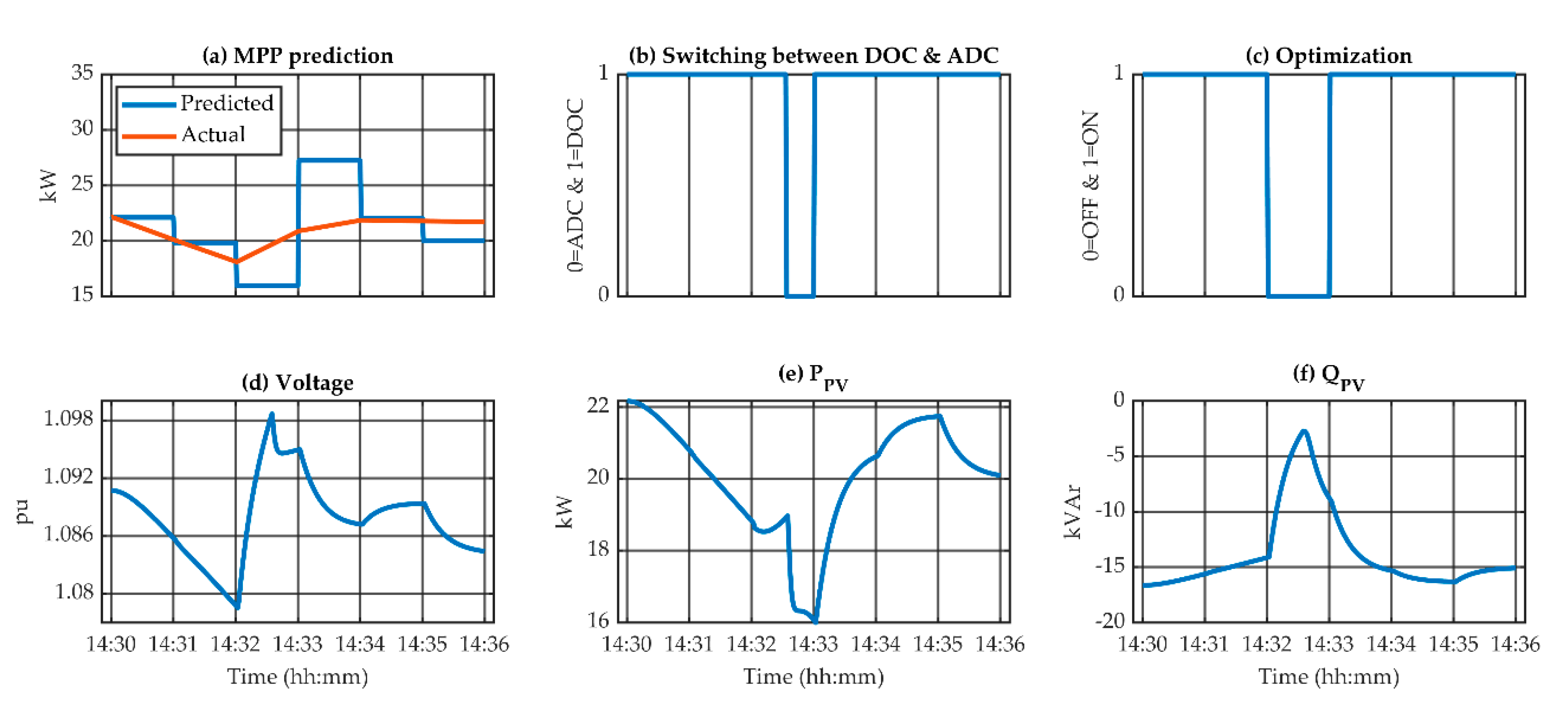
To show how the control system reacts in the event of prediction errors, a profile of a single PV inverter is selected for illustration. Figure 18 shows a selected profile of PV5 in simulation Case 2. As seen in Figure 17a, PV5 is switched from DOC to ADC at 2:32 pm. Additionally, in Case 2 of Figure 16, the optimization is not applied for a short time around 2:32 pm.

In Figure 18a, the prediction of the MPP profile is around 3.5 kW lower than the actual value at the time section of 2:32 to 2:33 pm, so that based on the predicted power flow analysis (block 5b of Figure 2b), the DOC turns off the optimization (block 6b of Figure 2b) and operates MPP (block 7b of Figure 2b), as seen in Figure 18c. Within the MPP operation (block 7b of Figure 2b), the reactive power of the PV5 is set to return to zero, leading to the reduction of the reactive power consumption and causing a voltage increase as seen in Figure 18d,18f. When the voltage exceeds 1.098 pu, the inverter switches from DOC to ADC, as seen in Figure 18b, and remains in this mode until the start of the next minute. During the time of running the ADC, the reactive power consumption is increased and the active power is reduced to maintain the voltage within network limits.

At the time section of 2:33 to 2:34 pm, the DOC predicts a solar power that is approximately 5.8 kW higher than reality, so that the predicted power flow voltage is higher than 1.095 pu (block 5b of Figure 2b), leading to the turning on of the DOC, as in Figure 18c. More reactive power is consumed, leading to a reduction in the voltage level.

The virtual loads applied in this research solve the need to know all information of devices outside the controllable area. This reduces not only the calculation power for the controller but also the communication system. The information of the virtual load is the total power (active and reactive) that flows through a bus. The virtual load may have the property of voltage dependence, but in this research, it is considered as a constant power load for the power flow analysis.

The voltage limit in the DOC is 1.095 pu, which is lower than 1.1 pu. The lower voltage limit causes higher active power curtailment. As explained before, the voltage limit for optimization calculation is chosen as being 0.005 pu less than the network threshold of 1.1 pu to allow for any optimization and prediction error. If there is an optimization error causing the bus voltage to be over 1.098 pu, the inverter would be switched back to the ADC to make sure that the voltage limit is not violated. If the voltage limit of DOC is set to be 1.1 pu, in the case of any error and when the voltage limit is violated, the inverter has to be shut down immediately. This would result in the hunting effect of turning on and off the inverter continuously.

6. Conclusions

This paper has presented a DOC using prediction and optimization. The PV inverter limits, including the power capacity and power factor, are considered. The control strategies have been verified by the MATLAB simulation of five different scenarios.

The ADC, in combination with the first-order filter, has been proven to be reliable and effective in avoiding overvoltage and the hunting effect. The ADC also considers the power factor limit and capacity of PV inverters.

The mechanism for the power flow analysis of a group of PV inverters inside a distribution network using the prediction method was introduced. The power flow calculation method using a virtual loads approach is applied to the controller to reduce the prediction calculation and the need to know all devices in a network.

A mechanism to switch between the DOC and ADC of a smart inverter is investigated to ensure network stability even in the event of erroneous optimal calculation and loss of communication. The DOC with a combination of a short time prediction, group optimization and virtual load can be applied for multiple and different groups in the network. This technique can also be applied for optimization of loss communication between controllable devices in further research.