Spatio-Temporal and Power–Energy Scheduling of Mobile Battery Storage for Mitigating Wind and Solar Energy Curtailment in Distribution Networks

Abstract

Several technical, computational, and economic barriers have caused curtailing a share of renewable-based power generation, especially in systems with higher penetration levels. The Mobile Battery Energy Storage (MBES) can cope with this problem considering the spatial and temporal distribution of the curtailed energy. Accordingly, a new operation model is proposed for optimal scheduling of the MBES in a distribution network with wind and photovoltaic (PV) resources. The network experiences curtailment situations because of bus overvoltage, feeder overload, and power over-generation. The MBES is a truck-mounted battery system compacted in a container. The proposed model seeks to determine the optimal spatio-temporal and power–energy status of the MBES to achieve a minimum curtailment ratio. The model considers transportation time and cost of the MBES efficiently while both active and reactive power exchanges are modeled. The model is linear, without convergence and optimality problems, applicable to real-life large-scale networks, and can be easily integrated into the commercial distribution management software. The implementation results on a test system demonstrate its functionality to recover a considerable share of the curtailed energy for both wind and PV resources at all curtailment patterns and scenarios.

1. Introduction

The growing share of renewable energy in the electricity generation portfolio has reduced energy costs in addition to air pollution [1]. However, some technical, economic, and computational limitations have restricted the maximum utilization of these clean and inexhaustible alternative energy resources. These restrictions have caused a percentage of renewable energy production to be cut off inevitably. Today, the imposed curtailment of renewable energy has become one of the main challenges in maximizing the deployment of these resources [2]. Regarding the high share in the total renewable generation, wind and solar constitute the highest global curtailment rates [3]. Only in China, 15.85% of wind and solar energy was curtailed in 2019. This value for Germany was 4.1 and 3.9 in 2017 and 2018, respectively. Moreover, the curtailed wind and solar energy touched 961 GWh in 2019 for California Independent System Operator (CAISO) [4]. Renewable energy curtailment often occurs during peak production or low-demand periods. The main reasons for forced cut-off are renewable potential and demand forecasting errors, electricity market economics and contracts frameworks, or grid limitations, including congestion, voltage rise, stability limits, or low flexibility. In addition to the economic consequences, the imposed cut of clean generation will also lead to environmental issues due to reduced renewable penetration [5]. To date, various methods have been proposed for mitigating renewable curtailment. Generally, these methods can be categorized as sector coupling via power-to-x [6], stationary energy storage [7], upgrading the grid, enhancing flexibility, defining supportive energy policies, and improving renewable energy and demand forecasting accuracy [8].

Recently, the idea of transporting battery energy storage to enhance grid applications was proposed. The mobile or transportable battery energy storage is a combination of the battery cells, power converter, and a transformer (if needed), all placed in a container on a truck or train. The whole system also comprises some battery management systems, automation, and protection devices [9,10,11]. The Mobile Battery Energy Storage (MBES) operation is constrained to the transportation time and the cost [12]. The spatio-temporal operation possibility of the MBES can offer various benefits for the grid and the consumers. Accordingly, the MBES based on railroad transportation was employed for congestion management [13], enhancing grid security [14], and uncertainty management of renewable resources [15]. The researchers in [16] used the MBES for multi-service provision in the distribution network, including price arbitrage, expansion deferral, and reactive power support. Enhancing the distribution grid’s resiliency during severe outages is the most focused application of the MBES in the literature. To this end, the MBES is used to form multiple microgrids coordinated with network reconfiguration to enhance the distribution grids’ resiliency. Accordingly, a two-stage model was proposed in [17] to optimize MBES investment in distribution networks, aiming to minimize expected load shedding. The model forms dynamic microgrids to cope with disasters. The optimal MBES capacity is determined in the first stage, while spatio-temporal status will be determined optimally in the second stage. A post-disaster restoration procedure was proposed in [18] by coordinating and optimizing the MBES and generation resources in the microgrids and network reconfiguration to achieve a minimum operation schedule. Besides, the MBES and an electric vehicle fleet were used in [19] to boost the distribution grid’s resiliency. Coordination of the network repair crew and mobile generators scheduling with the MBES was addressed in [20] via proposing a new model for optimizing service restoration in distribution networks.

In [21], a two-stage stochastic model based on the user-equilibrium-based multi-layer multi-timescale time-space network was proposed for maximum utilization of the MBES mobility under variable resources and transportation traffic uncertainties. The model aims to minimize the system’s expected operation cost by enhancing the flexibility of coupled transmission and distribution networks and hybrid AC/DC microgrids’ conversion capacities. The authors in [22] focused on a network-constrained robust unit commitment model integrating MBES and demand response programs. The information gap decision theory was employed to cope with wind energy uncertainty. The optimal sizing of the MBES for the provision of multiple services in the distribution network is addressed in [23]. The proposed model takes load variations, renewable intermittency, and market price fluctuations into account while the battery’s capacity and lifetime constraints are modeled. Finally, the authors in [24] proposed a two-stage robust-stochastic market-clearing model while considering rail-based battery storage transportation in the transmission network. Besides, a demand response program, price-sensitive shiftable load bidding, is applied to increase the network’s flexibility and environmental performance.

The distribution of renewable energy curtailment in the grid varies both temporally and spatially. Solar and wind energy currently constitute the most dominant grid integrated renewable energies and thus have the highest curtailment rate. Fortunately, the time distribution of their maximum energy output period is almost different. As a result, the MBES can be present at different time periods to store the curtailed energy at different production locations. This application of the MBES was focused on in this paper. The application of the MBES for renewable curtailment mitigation was addressed previously as a by-product of the other applications. Moreover, various curtailment causes and scenarios and the applicability of the MBES to recover the curtailed energy at each one are not addressed yet. With this view, a new MBES transportation model is proposed in this paper for renewable curtailment mitigation. The proposed model is utterly different from the previous formulations. The proposed model considers transportation time and cost of the MBES efficiently and with less computational burden. The model is linear, while the reactive power exchange of the battery is taken into account besides the active power. The only model inputs are the time and cost of transporting the MBES between network buses. Reactive power flow and bus voltages are also considered via linear equations to preserve the whole model’s linearity. The proposed model is integrated into the distribution grid Optimal Power Flow (OPF) to mitigate solar and wind energy curtailment. Three primary technical reasons for the imposed cut-off of these resources in the distribution network are considered. In other words, the applicability of the MBES utilizing the proposed method to mitigate renewable energy curtailment caused by the power over-generation, feeder overload, and bus overvoltage is analyzed. Concisely, the paper novelties are:

-

Proposing a spatio-temporal and power–energy scheduling model for truck-mounted mobile battery in distribution networks while considering transportation time and cost;

-

Constructing a linear model taking battery reactive power exchange and full power factor range into account;

-

Validating the proposed MBES model functionality to recover a considerable share of the curtailed energy for both wind and PV resources at all curtailment patterns and scenarios.

The rest of the paper is organized as follows. In Section 2, the proposed model for MBES operation is outlined and formulated. The case study is implemented in Section 3, wherein results and discussions are provided. Finally, the concluding remarks of the study are drawn in Section 4.

2. Proposed Model for Mobile Battery Operation

The Mobile Battery Energy Storage (MBES) is a complete battery system placed in a container capable of transportation using any shipping method. Accordingly, the MBES can be charged or discharged at any preferred location in the network when needed. The truck-mounted MBES is the most proposed MBES realization method, especially in the distribution network. Road-based battery transportation is consistent with the battery sizes suitable for operation in distribution networks and offers more flexibility in transportation time [25]. An illustrative example is used to describe the proposed MBES operation model. 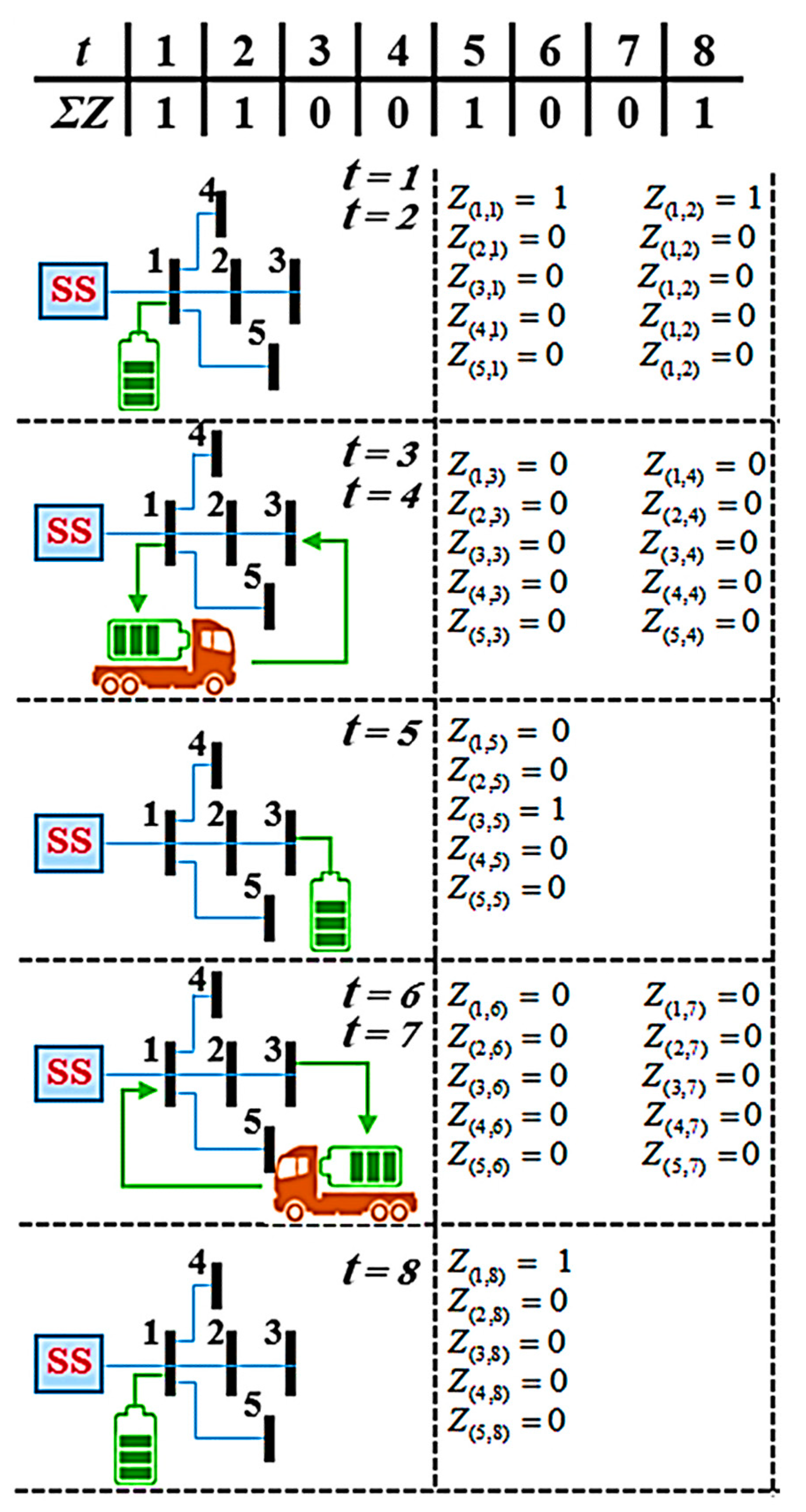A simple distribution network (DN) with five buses connected to the upstream substation (SS) is considered in Figure 1. The DN has an MBES, and eight one-hour time periods are considered. It is assumed that the MBES is at Bus #1 for two first hours for charging. Then, it is transported during the third and fourth hours. It will be at Bus #2 at the fifth hour for discharging. Subsequently, it transports during the sixth and seventh hours to be at its initial place, Bus # 1, at the last hour. The transportation method is based on the road network. The transportation network is mapped into the distribution network in the coincidence points, i.e., network buses. In the points where the transportation network crosses a distribution network bus, and there is access to the truck’s parking footprint, a parking station for MBES is assigned.

2.1. Primary Rules of MBES Operation

A binary variable can be used to present the spatio-temporal status of the MBES. This binary variable, Z(i,t), indicates the presence of the MBES in the bus i and at time period t. Accordingly, when the MBES is connected to the grid for the charging and discharging, the variable’s value is one, and when transporting between the buses, its value must be zero. Corresponding values for Z(i,t) are shown in Figure 1 for all time periods and DN buses. The first MBES operation limitation is that it can connect to only one of the network buses at any time, as formulated in Equation (1). If the sum of all Z(i,t) is zero for a time period, it means the MBES was being transported at that period. Accordingly, the MBES is transported during hours 3,4,6, and 7 in this illustrative example. Another point is that the initial status of the MBES has to be determined previously. At the beginning of the daily scheduling, the spatio-temporal binary status of the MEBS is equal to this predefined situation, as denoted by Equation (2). Similarly, at the end of the time periods, the MBES has to be relocated to the initial location to start a day ahead, as denoted by Equation (3). These constraints are also consistent with the example wherein the MBES starts from Bus #1 and relocates to that place at the end of the time periods, as depicted in Figure 1.

$${\displaystyle \sum _i{Z}_{\left(i,t\right)}^{}}\le 1\hspace{0.17em}\hspace{0.17em}\hspace{0.17em}\hspace{0.17em}\hspace{0.17em}\hspace{0.17em}\forall t$$

(1)

$$Z_{\left(j,u\right)}^{}=Z_{\left(i,t\right)}^0\hspace{0.17em}\hspace{0.17em}\hspace{0.17em}\forall i,j,t,u=t_0$$

(2)

$$Z_{\left(j,u\right)}^{}=Z_{\left(i,t\right)}^0\hspace{0.17em}\hspace{0.17em}\hspace{0.17em}\forall i,j,t,u=T$$

(3)

2.2. Transportation Time Modelling

Since the MBES must disconnect its electrical connection before leaving the bus, a specific time has to be spent for this purpose. Similarly, after the MBES reaches the new location, its operation requires spending a specific time for bus reconnection. These two times, disconnection time and reconnection time, together with the time required for traveling the distance between the two buses, will constitute the total MBES transportation time. The total MBES transportation time is a specific value for each movement between network buses. The corresponding values, i.e., Transportation Time (TTij), can be presented by a matrix such as Equation (4). The MBES transportation time for the illustrative example depicted in Figure 1 is supposed to be Equation (5).

$$TT=\left[\begin{array}{l}0\hspace{0.17em}\hspace{0.17em}\hspace{0.17em}\hspace{0.17em}\hspace{0.17em}\hspace{0.17em}\hspace{0.17em}\hspace{0.17em}\hspace{0.17em}\hspace{0.17em}T{T}_{1,2}\hspace{0.17em}\dots \hspace{0.17em}T{T}_{1,J}\\ T{T}_{2,1}\hspace{0.17em}\hspace{0.17em}\hspace{0.17em}\hspace{0.17em}\hspace{0.17em}\hspace{0.17em}\hspace{0.17em}0\hspace{0.17em}\hspace{0.17em}\hspace{0.17em}\hspace{0.17em}\hspace{0.17em}\hspace{0.17em}\hspace{0.17em}\hspace{0.17em}\hspace{0.17em}\hspace{0.17em}\hspace{0.17em}\hspace{0.17em}⋮\hspace{0.17em}\hspace{0.17em}\hspace{0.17em}\\ \hspace{0.17em}\hspace{0.17em}\hspace{0.17em}\cdots \hspace{0.17em}\hspace{0.17em}\hspace{0.17em}\hspace{0.17em}\hspace{0.17em}\hspace{0.17em}\hspace{0.17em}\hspace{0.17em}\hspace{0.17em}\hspace{0.17em}\hspace{0.17em}\hspace{0.17em}\hspace{0.17em}\hspace{0.17em}\hspace{0.17em}0\hspace{0.17em}\hspace{0.17em}\hspace{0.17em}\hspace{0.17em}\hspace{0.17em}⋮\hspace{0.17em}\\ T{T}_{I,1}\hspace{0.17em}\hspace{0.17em}\hspace{0.17em}\hspace{0.17em}\hspace{0.17em}\hspace{0.17em}\cdots \hspace{0.17em}\hspace{0.17em}\hspace{0.17em}\hspace{0.17em}\hspace{0.17em}\hspace{0.17em}\hspace{0.17em}\hspace{0.17em}\hspace{0.17em}\hspace{0.17em}\hspace{0.17em}\hspace{0.17em}0\end{array}\right]\hspace{0.17em}\hspace{0.17em}\forall \hspace{0.17em}\hspace{0.17em}i,j$$

(4)

$$TT{\hspace{0.17em}}^{[h]}=\left[\begin{array}{l}0\hspace{0.17em}\hspace{0.17em}1\hspace{0.17em}\hspace{0.17em}2\hspace{0.17em}\hspace{0.17em}3\hspace{0.17em}\hspace{0.17em}4\\ 1\hspace{0.17em}\hspace{0.17em}0\hspace{0.17em}\hspace{0.17em}1\hspace{0.17em}\hspace{0.17em}2\hspace{0.17em}\hspace{0.17em}3\\ 2\hspace{0.17em}\hspace{0.17em}1\hspace{0.17em}\hspace{0.17em}0\hspace{0.17em}\hspace{0.17em}1\hspace{0.17em}\hspace{0.17em}2\\ 3\hspace{0.17em}\hspace{0.17em}2\hspace{0.17em}\hspace{0.17em}1\hspace{0.17em}\hspace{0.17em}0\hspace{0.17em}\hspace{0.17em}1\\ 4\hspace{0.17em}\hspace{0.17em}3\hspace{0.17em}\hspace{0.17em}2\hspace{0.17em}\hspace{0.17em}1\hspace{0.17em}\hspace{0.17em}0\end{array}\right]\hspace{0.17em}\hspace{0.17em}\hspace{0.17em}\hspace{0.17em}\hspace{0.17em}\hspace{0.17em}\forall \hspace{0.17em}\hspace{0.17em}i,j$$

(5)

The necessary condition for transporting the MBES between different buses is that the travel time between the origin and destination bus has elapsed. It must be kept in mind that if the MBES is currently connected to bus i, it must not be connected to the grid for a certain period of time to connect to another bus rather than i at a later time. In other words, if the MBES connection bus will change in the future, the Z(i,t) must be zero in some next time intervals. The number of the time intervals wherein the Z(i,t) must be kept zero depends on the destination bus and, consequently, its transportation time from the origin bus. In our example, the transportation time between Bus #1 and Bus #3 is two hours. The MBES is disconnected from the grid and on the road for two hours (hours 3 and 4). This limitation on connection is modeled by Equation (6). The inequality denotes that if the origin and destination buses are not the same, the destination bus’s binary variable cannot be switched on at least before the required transportation time has elapsed.

$$Z_{\left(i,t\right)}^{MB}+Z_{\left(j,u\right)}^{MB}\le 1\hspace{0.17em}\hspace{0.17em}\hspace{0.17em}\hspace{0.17em}\forall i,j,t,i\ne j,u=\left\{\hspace{0.17em}t+1,\dots ,t+T{T}_{\left(i,j\right)}\right\}$$

(6)

In the illustrative example, considering that Z(1,2) = 1 and the MBES needs to be at Bus #3 for discharging, the inequality enforces that for t = 3 and t = 4, all binary variables should be zero. This case is also valid for the second transportation from Z(3,5) to Z(1,8), wherein Z(i,6) and Z(i,7) are all zero. The above inequality ensures elapsing transportation time between buses. However, it does not necessitate that the MBES be connected to the grid after passing this time. In this case, the MBES may experience some unnecessary idle status without network connection after transportation. This problem is handled by adding inequality Equation (7). The constraint imposes that the destination bus’s status binary variable has to be switched on if the required transportation time from the origin bus is elapsed.

$${\displaystyle \sum _{u\hspace{0.17em}=\hspace{0.17em}\hspace{0.17em}t+1}^{t+T{T}_{\left(i,j\right)}+1}\left[Z_{\left(j,u\right)}^{}\right]}\ge \hspace{0.17em}\hspace{0.17em}\hspace{0.17em}{Z}_{\left(i,t\right)}^{}\hspace{0.17em}\hspace{0.17em}\hspace{0.17em}\forall i,j,t,i\ne j,u=\left\{\hspace{0.17em}t+1,\dots ,t+T{T}_{\left(i,j\right)}\right\}$$

(7)

2.3. Transportation Cost Modelling

Transporting the MBES between network buses necessitates a certain cost. For a truck-mounted MBES, this cost is composed of the driver and electrical technician crew cost, truck renting cost, and fuel cost. The daily operation cost of the MBES is a function of the performed transportations during the whole day. The battery operation cost for each movement between network buses is a specific value. The corresponding values, i.e., Transportation Cost (TCij), can be presented in a matrix such as Equation (8). The MBES transportation cost for the illustrative example depicted in Figure 1 is supposed to be as Equation (9).

$$TC=\left[\begin{array}{l}0\hspace{0.17em}\hspace{0.17em}\hspace{0.17em}\hspace{0.17em}\hspace{0.17em}\hspace{0.17em}\hspace{0.17em}\hspace{0.17em}\hspace{0.17em}\hspace{0.17em}T{C}_{1,2}\hspace{0.17em}\dots \hspace{0.17em}T{C}_{1,J}\\ T{C}_{2,1}\hspace{0.17em}\hspace{0.17em}\hspace{0.17em}\hspace{0.17em}\hspace{0.17em}\hspace{0.17em}\hspace{0.17em}0\hspace{0.17em}\hspace{0.17em}\hspace{0.17em}\hspace{0.17em}\hspace{0.17em}\hspace{0.17em}\hspace{0.17em}\hspace{0.17em}\hspace{0.17em}\hspace{0.17em}⋮\hspace{0.17em}\hspace{0.17em}\hspace{0.17em}\\ \hspace{0.17em}\hspace{0.17em}\hspace{0.17em}\cdots \hspace{0.17em}\hspace{0.17em}\hspace{0.17em}\hspace{0.17em}\hspace{0.17em}\hspace{0.17em}\hspace{0.17em}\hspace{0.17em}\hspace{0.17em}\hspace{0.17em}\hspace{0.17em}\hspace{0.17em}\hspace{0.17em}\hspace{0.17em}\hspace{0.17em}0\hspace{0.17em}\hspace{0.17em}\hspace{0.17em}⋮\hspace{0.17em}\\ T{C}_{I,1}\hspace{0.17em}\hspace{0.17em}\hspace{0.17em}\hspace{0.17em}\hspace{0.17em}\hspace{0.17em}\cdots \hspace{0.17em}\hspace{0.17em}\hspace{0.17em}\hspace{0.17em}\hspace{0.17em}\hspace{0.17em}\hspace{0.17em}\hspace{0.17em}\hspace{0.17em}\hspace{0.17em}0\end{array}\right]\hspace{0.17em}\hspace{0.17em}\forall \hspace{0.17em}\hspace{0.17em}i,j$$

(8)

$$TT{\hspace{0.17em}}^{[\$]}=\left[\begin{array}{l}0\hspace{0.17em}\hspace{0.17em}\hspace{0.17em}\hspace{0.17em}10\hspace{0.17em}\hspace{0.17em}\hspace{0.17em}20\hspace{0.17em}\hspace{0.17em}\hspace{0.17em}30\hspace{0.17em}\hspace{0.17em}\hspace{0.17em}40\\ 10\hspace{0.17em}\hspace{0.17em}\hspace{0.17em}0\hspace{0.17em}\hspace{0.17em}\hspace{0.17em}\hspace{0.17em}10\hspace{0.17em}\hspace{0.17em}\hspace{0.17em}20\hspace{0.17em}\hspace{0.17em}\hspace{0.17em}30\\ 20\hspace{0.17em}\hspace{0.17em}\hspace{0.17em}10\hspace{0.17em}\hspace{0.17em}\hspace{0.17em}0\hspace{0.17em}\hspace{0.17em}\hspace{0.17em}\hspace{0.17em}10\hspace{0.17em}\hspace{0.17em}\hspace{0.17em}20\\ 30\hspace{0.17em}\hspace{0.17em}\hspace{0.17em}20\hspace{0.17em}\hspace{0.17em}\hspace{0.17em}10\hspace{0.17em}\hspace{0.17em}\hspace{0.17em}0\hspace{0.17em}\hspace{0.17em}\hspace{0.17em}\hspace{0.17em}10\\ 40\hspace{0.17em}\hspace{0.17em}\hspace{0.17em}30\hspace{0.17em}\hspace{0.17em}\hspace{0.17em}20\hspace{0.17em}\hspace{0.17em}\hspace{0.17em}10\hspace{0.17em}\hspace{0.17em}\hspace{0.17em}0\end{array}\right]\hspace{0.17em}\hspace{0.17em}\hspace{0.17em}\hspace{0.17em}\hspace{0.17em}\hspace{0.17em}\forall \hspace{0.17em}\hspace{0.17em}i,j$$

(9)

A binary indicator variable is used to model MBES transportation. This binary variable denotes transportation from bus i and at time period t (Z(i,t)) to bus j and at time period u (Z(j,u)), where u = t + TT(i,j) + 1 and i≠j. This variable can be calculated by multiplying the origin and destination status binary variable, as presented by Equation (10).

$$T_{\left(i,j,t,u\right)}=Z_{\left(i,t\right)}^{}\hspace{0.17em}{Z}_{\left(j,u\right)}^{}\hspace{0.17em}\hspace{0.17em}\hspace{0.17em}\forall i,j,t,i\ne j\hspace{0.17em},\hspace{0.17em}\hspace{0.17em}u=\left\{\hspace{0.17em}t+T{T}_{(i,j)}+1\right\}\hspace{0.17em}\hspace{0.17em}$$

(10)

In our example, the origin status variable is one for the first hour; however, all possible destination variables are zero. Therefore, no transportation has occurred. For the second hour, the origin status variable and the status variable at the fifth hour for Bus #3 are one. Hence, the corresponding transportation variable, T(1,3,2,5), will be equal to one indicating the MBES transportation. For hours 3,4,6, and 7, the transportation variable will be equal to zero, considering that the origin bus’s binary status variable is zero for all the buses.

There will be another transportation initiated after hour 5 and from Bus #3. In this case, the MBES has four transportation choices with a destination at hour 7 and hour 8, as illustrated in Figure 1. Finally, the MBES is turned back to Bus #1 at hour 8. As a result, second transportation is calculated as T(3,1,5,8). The non-linearity caused by the multiplication in Equation (10) can be alleviated by transforming to Equations (11–13). The MBES transportation cost for each movement can be calculated by multiplying the transportation indicator variable by corresponding transportation cost, denoted by Equation (14). For the illustrative example, daily MBES operation costs a total value of 40 $, transportation cost for Bus #1 to Bus #3 movement (20$) and vice versa (20$).

$$T_{\left(i,j,t,u\right)}\ge Z_{\left(i,t\right)}^{}+Z_{\left(j,u\right)}^{}-1\hspace{0.17em}\hspace{0.17em}\hspace{0.17em}\forall i,j,t,i\ne j,u=\left\{\hspace{0.17em}t+T{T}_{(i,j)}+1\right\}\hspace{0.17em}\hspace{0.17em}$$

(11)

$$T_{\left(i,j,t,u\right)}\le Z_{\left(i,t\right)}^{}\hspace{0.17em}\hspace{0.17em}\hspace{0.17em}\forall i,j,t,i\ne j,u=\left\{\hspace{0.17em}t+T{T}_{(i,j)}+1\right\}$$

(12)

$$T_{\left(i,j,t,u\right)}\le Z_{\left(j,t\right)}^{}\hspace{0.17em}\hspace{0.17em}\hspace{0.17em}\forall i,j,t,i\ne j,u=\left\{\hspace{0.17em}t+T{T}_{(i,j)}+1\right\}$$

(13)

$$T{C}_{\left(i,j,t,u\right)}^{MB}=T_{\left(i,j,t,u\right)}T{C}_{\left(i,j\right)}\hspace{0.17em}\hspace{0.17em}\hspace{0.17em}\hspace{0.17em}\hspace{0.17em}\hspace{0.17em}\hspace{0.17em}\hspace{0.17em}\hspace{0.17em}\hspace{0.17em}\hspace{0.17em}\forall i,j,t,u$$

(14)

2.4. Power and Energy Constraints

The general limitations on a generic battery systems operation have to be adapted to be used with the proposed MBES model. The first one is that the battery cannot be charged and discharged simultaneously. Besides, each charge and discharge power passing the battery cannot exceed its nominal power. These constraints are modeled by using indicator charging and discharging binary variables as in Equations (15)–(17) [26]. It should be noted that charging and discharging of the MBES in a bus at a specific time period depends on its presence at that time and location, or in other words, the unity of the relevant spatio-temporal binary variable. These limitations are also valid for the inductive and capacitive reactive power contribution of the battery, which is modeled in Equations (18–20) in a similar way to the active power. Last but not least, the apparent power flow limit of the MBES in Equation (21) is considered by a piece-wise linearization method to avoid non-linearity.

$$X_{(i,t)}^{CP}+X_{(i,t)}^{DP}\le Z_{(i,t)}^{}\hspace{0.17em}\hspace{0.17em}\hspace{0.17em}\forall i,t$$

(15)

$$p_{(i,t)}^{BC}\le X_{(i,t)}^{CP}\hspace{0.17em}{S}_{MB}^R\hspace{0.17em}\hspace{0.17em}\hspace{0.17em}\forall i,t$$

(16)

$$p_{(i,t)}^{BD}\le X_{(i,t)}^{DP}\hspace{0.17em}{S}_{MB}^R\hspace{0.17em}\hspace{0.17em}\hspace{0.17em}\forall i,t$$

(17)

$$Y_{(i,t)}^{IQ}+Y_{(i,t)}^{CQ}\le Z_{(i,t)}^{}\hspace{0.17em}\hspace{0.17em}\hspace{0.17em}\forall i,t$$

(18)

$$q_{(i,t)}^{BI}\le Y_{(i,t)}^{IQ}\hspace{0.17em}{S}_{MB}^R\hspace{0.17em}\hspace{0.17em}\hspace{0.17em}\forall i,t$$

(19)

$$q_{(i,t)}^{BC}\le Y_{(i,t)}^{CQ}\hspace{0.17em}{S}_{MB}^R\hspace{0.17em}\hspace{0.17em}\hspace{0.17em}\forall i,t$$

(20)

$${\left(p_{(i,t)}^{BC}+p_{(i,t)}^{BD}\right)}^2+{\left(q_{(i,t)}^{BI}+q_{(i,t)}^{BC}\right)}^2\le \hspace{0.17em}{\left(S_{MB}^R\right)}^2\hspace{0.17em}\hspace{0.17em}\hspace{0.17em}\forall i,t$$

(21)

The energy stored in the battery has to be kept within the permissible values formulated in Equation (22). The stored energy is a function of the previously stored value and the performed charging and discharging regarding related efficiencies, as modeled by Equation (23). The critical point to be noticed in this equation is that the summation over net charged and discharged powers will only gather the power at the MBES connection bus. The last constraint on the battery energy is that the net absorbed and released energy during the whole operation time periods should be the same, which is denoted by Equation (24) [27].

$$E_{MB}^{Min}\le e_{\left(t\right)}^{MB}\le \hspace{0.17em}{E}_{MB}^{Max}\hspace{0.17em}\hspace{0.17em}\hspace{0.17em}\hspace{0.17em}\hspace{0.17em}\forall t$$

(22)

$$e_{\left(t\right)}^{MB}=e_{(t-1)}^{MB}+{\displaystyle \sum _i{p}_{\left(i,t\right)}^{BC}{\eta }_{}^{BC}}-{\displaystyle \sum _i{p}_{\left(i,t\right)}^{BD}/{\eta }_{}^{BD}}\hspace{0.17em}\hspace{0.17em}\hspace{0.17em}\hspace{0.17em}\forall t$$

(23)

$${\displaystyle \sum _{(i,t)}{p}_{\left(i,t\right)}^{BC}{\eta }_{}^{BC}}={\displaystyle \sum _{(i,t)}{p}_{\left(i,t\right)}^{BD}/{\eta }_{}^{BD}}$$

(24)

2.5. MBES Model Inclusion in Distriution OPF

The proposed mathematical model for the MBES operation is integrated into the optimal power flow (OPF) framework of the distribution network. To this end, the linear version of the DistFlow equations, known as LinDistFlow, is used. Details of the LinDistFlow can be found in [28]. The previously proposed OPF model is employed in this study with a modification in the bus power balance equation. The charging and discharging power of the MBES were emulated by adding a corresponding fictitious load and generation in the bus. Accordingly, the balance of the active and reactive power flow in any network bus is shown by Equations (25) and (26). In this equation, the MBES’ active charge and discharge powers are treated as the fictitious load and generation. The inductive and capacitive reactive power of the MBES are also handled similarly. The apparent power flow of network lines has to be lower than the thermal capacity, denoted by Equation (27). This non-linear constraint is handled similarly to the MBES flow using piece-wise linearization. Finally, from the total active power generated from the distributed renewable resource, a portion is used in the grid, and the remaining one is curtailed inevitably, as it is formulated by Equation (28).

$${\displaystyle \sum _i{p}_{(i,j,t)}^{Flow}}\hspace{0.17em}+p_{(j,t)}^{BC}+\hspace{0.17em}{p}_{(j,t)}^{DG}=\hspace{0.17em}{\displaystyle \sum _k{p}_{(j,k,t)}^{Flow}}\hspace{0.17em}+p_{(j,t)}^{BD}+\hspace{0.17em}{P}_{(j,t)}^{LD}\hspace{0.17em}\hspace{0.17em}\hspace{0.17em}\forall j,t$$

(25)

$${\displaystyle \sum _i{q}_{(i,j,t)}^{Flow}}\hspace{0.17em}+q_{(j,t)}^{BI}+\hspace{0.17em}{q}_{(j,t)}^{DG}=\hspace{0.17em}{\displaystyle \sum _k{q}_{(j,k,t)}^{Flow}}\hspace{0.17em}+q_{(j,t)}^{BC}+\hspace{0.17em}{Q}_{(j,t)}^{LD}\hspace{0.17em}\hspace{0.17em}\hspace{0.17em}\forall j,t$$

(26)

$$p_{(i,j,t)}^{Flow}{}^2+q_{(i,j,t)}^{Flow}{}^2\le \hspace{0.17em}{\left(S_{(i,j)}^{Max}\right)}^2\hspace{0.17em}\hspace{0.17em}\hspace{0.17em}\forall i,\hspace{0.17em}t$$

(27)

$$c{p}_{(i,t)}^{DG}=c_{(i,t)}^{DG}+p_{(i,t)}^{DG}\hspace{0.17em}\hspace{0.17em}\hspace{0.17em}\forall i,\hspace{0.17em}t$$

(28)

The relation between sending and receiving bus voltages of each line, represented by Equation (29), is a function of the line’s parameters and active and reactive powers. The voltage magnitude of buses has to be within the permissible values, modeled by Equation (30). For the substation energy cost, a piece-wise linear approximation is assumed. In this way, the total hourly power drawn from the substation can be calculated using Equation (31).

$${\nu }_{\left(i,t\right)}={\nu }_{\left(j,t\right)}-2\hspace{0.17em}(R_{(i,j)}{p}_{(i,j,t)}^{Flow}+X_{(i,j)}{q}_{(i,j,t)}^{Flow})\hspace{0.17em}\hspace{0.17em}\hspace{0.17em}\forall i,j,t$$

(29)

$$V_{\min }\le {\nu }_{\left(i,t\right)}\le V_{\max }\hspace{0.17em}\hspace{0.17em}\hspace{0.17em}\forall i,t$$

(30)

$$P_{\left(t\right)}^{SS}={\displaystyle \sum _n^{}\mathsf{\Delta }{P}_{\left(n,t\right)}^{SS}}\hspace{0.17em}\hspace{0.17em}\hspace{0.17em}\hspace{0.17em}\forall t$$

(31)

The problem’s objective function is assigned to the sum of the substation energy cost with the MBES transportation cost over the daily operation’s entire time periods. Thus, the total daily operation cost can be shown by Equation (32).

$$Min\hspace{0.17em}\hspace{0.17em}\hspace{0.17em}O{C}^{Tot}={\displaystyle \sum _{(n,t)}^{}{\lambda }_{\left(n\right)}^{SS}\hspace{0.17em}\mathsf{\Delta }{P}_{\left(n,t\right)}^{SS}}+{\displaystyle \sum _{(i,j,t,u)}^{}T{C}_{\left(i,j,t,u\right)}^{MB}}$$

(32)

It should be noted that the considered objective function possesses a cost-based nature. Accordingly, the solution procedure seeks to obtain a minimum cost operation schedule. This orientation means that the curtailed renewable energy will be recovered if its cost is lower than the substation energy cost. In other words, the renewable resources have to be utility-owned generators and with zero operation cost. In this case, the problem will try to minimize curtailed energy by optimal scheduling of the MBES. The optimal scheduling means defining spatio-temporal and power–energy status of the MBES to yield the minimum renewable curtailment ratio.

3. Case Study

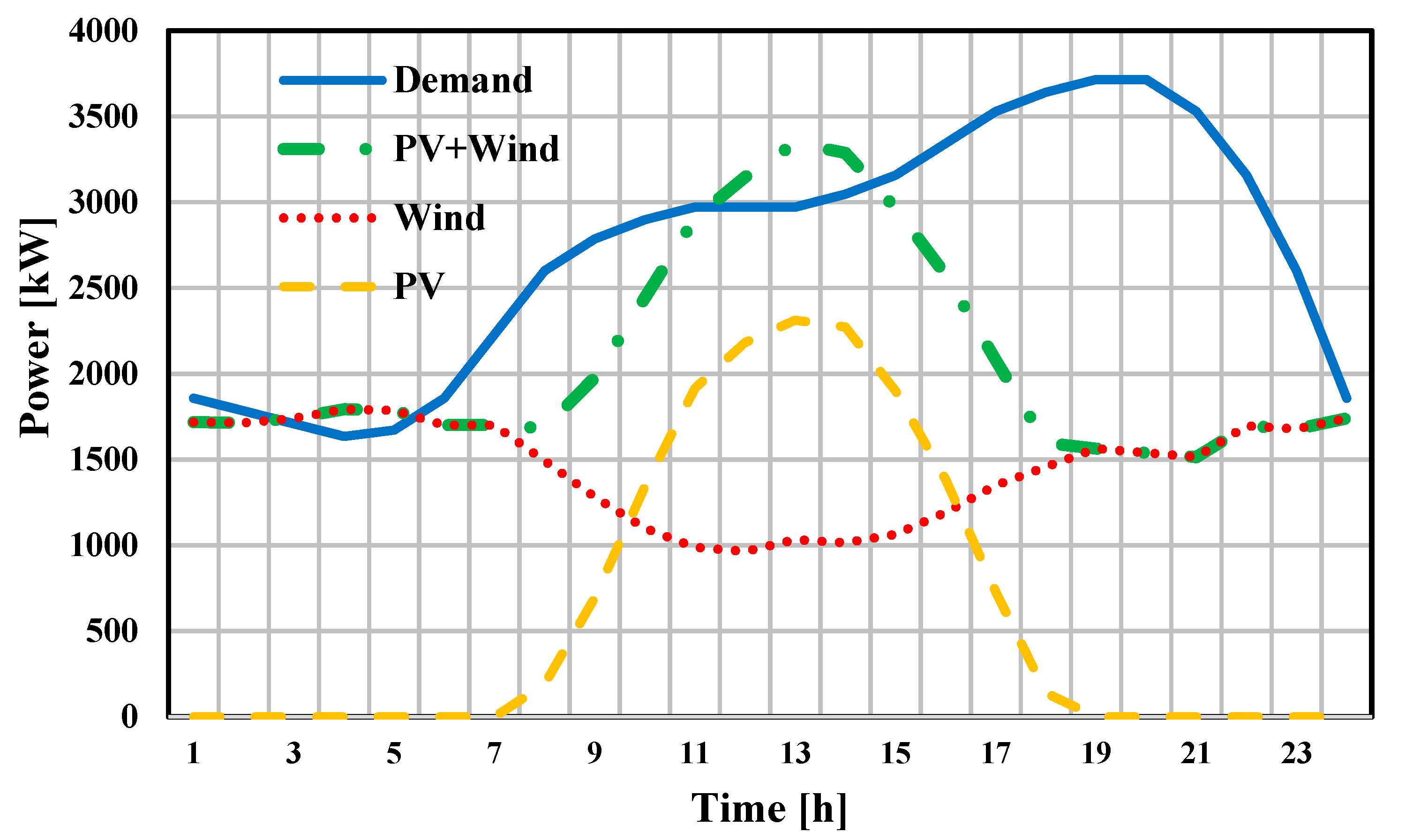
The model developed in the previous section is tested on the IEEE 33-bus distribution test system. The line and bus load data can be found in [29]. The distributed generation resources in the form of PV panels and wind turbines are added to buses 22 and 25. The hourly load and production profile for the wind farm, PV panels, and total renewable generation for the base case simulations are shown in Figure 2.

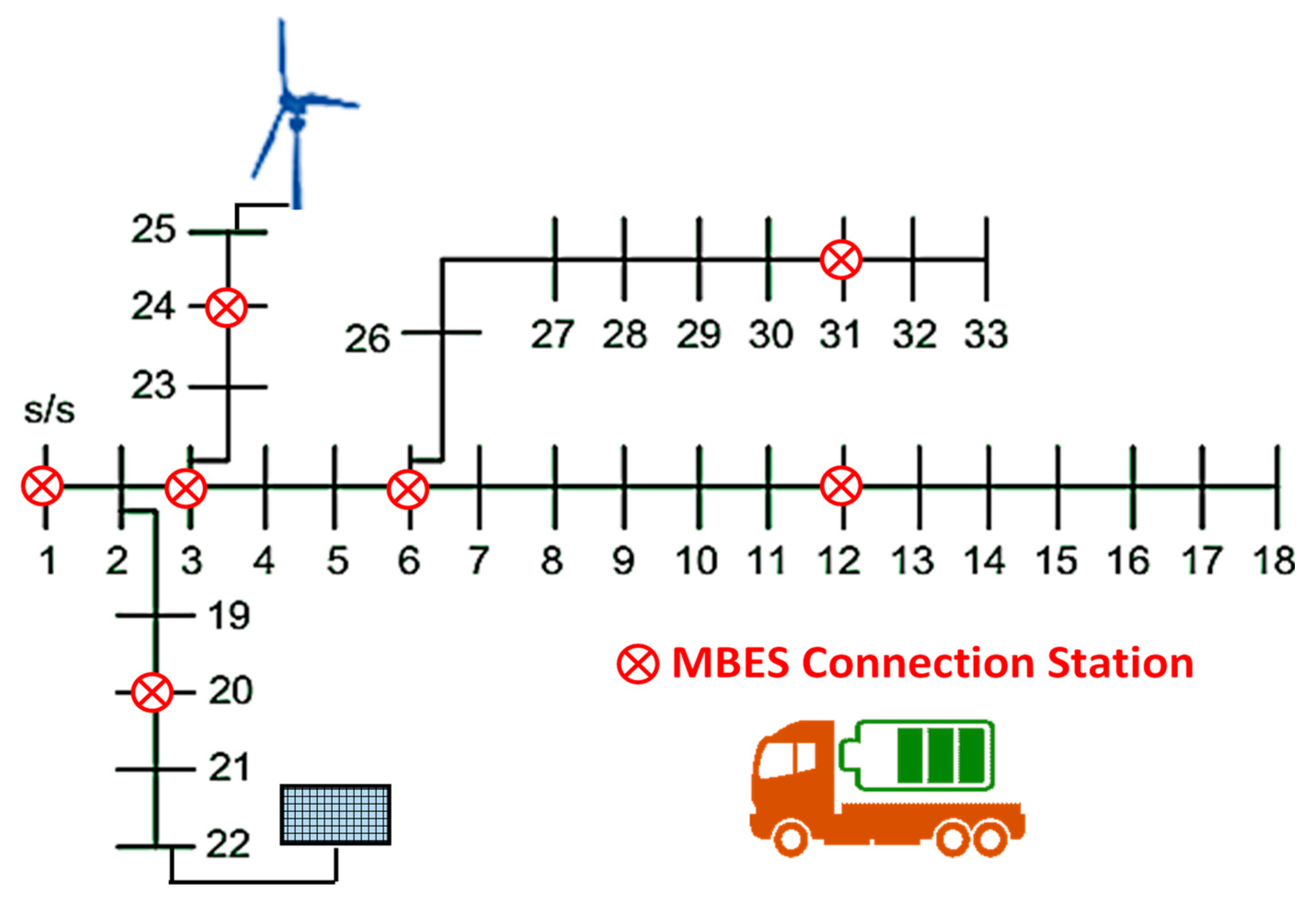
The system is equipped with an 800 kW and 2000 kWh MBES with the parking stations at buses 1, 3, 6, 12, 20, 24, 31, as depicted in Figure 3. Considering that the transportation network crosses the distribution network at limited and specific bus numbers and also truck parking location limitations, a limited number of network buses have the opportunity for MBES connection. The battery’s round-trip efficiency is equal to 0.9 while it starts the operation period with zero initial energy and is located at Bus #1.

Table 1. Transportation time of the MBES (h).

Bus	1	3	6	12	20	24	31
1	0	1	1	2	1	1	3
3	1	0	1	2	2	2	2
6	1	1	0	2	2	2	2
12	2	2	2	0	1	1	2
20	1	2	2	1	0	1	3
24	1	2	2	1	1	0	3
31	3	2	2	2	3	3	0

and

Table 2. Transportation cost of the MBES ($).

Bus	1	3	6	12	20	24	31
1	0	50	80	150	100	100	200
3	50	0	50	150	200	200	150
6	100	50	0	100	150	150	150
12	150	150	100	0	80	80	150
20	100	200	150	80	0	100	250
24	100	200	150	80	100	0	250
31	200	150	150	150	250	250	0

present the transportation time and cost of the MBES transportation between network buses, respectively.

Three different cases indicating various curtailment causes are simulated, including power over-generation, bus overvoltage, and feeder overload curtailment. Each case is itself composed of five scenarios.

Table 3. Details of the simulated cases.

Case Title	Curtailment Cause	Renewable Generation Factor	Voltage Deviation Limit	Line Thermal Capacity
Ogc	Power Over-generation	0.9–1.1	Free	Free
Ovc	Bus Overvoltage	1.00	0.05–0.15	Free
Olc	Line overload	1.00	Free	0.6–1.4

represents details of the controlled parameters for each simulation case. In the over-generation curtailment (Ogc), there is no limitation on the bus voltages in addition to the feeder capacity. In the Ogc case, the base wind and solar generation profile in Figure 3 is changed with a factor of 0.9 to 1.1. Then, each resource’s curtailment is calculated for the conventional distribution network (DN) and the network equipped with the mobile battery (MB).

For the overvoltage curtailment (Ovc), the renewable power generation is constant and based on Figure 2. Moreover, there is no line flow limit in the network. However, the bounds on the bus voltage are changed with a deviation from 5 to 15 percent, and then the curtailment is calculated. Finally, for the overload curtailment (Olc), the renewable profile is kept constant similar to the previous case. Additionally, the voltage limits for the network buses are not applied. In this case, the power rating of lines 3–23 (wind farm lateral) and 2–19 (PV site lateral) is first set to 1200 and 500 kVA, respectively. These ratings are then changed from 80 to 140 percent to calculate the effect of the congestion on the renewable curtailment.

Table 4. Simulation results for Ogc case.

Case Title			Ogc90	Ogc95	Ogc100	Ogc105	Ogc110
Total Operation Cost ($)		DN	4217	3757	3371	3017	2714
		MB	3620	3123	2656	2264	1892
		%	14.16	16.86	21.21	24.96	30.30
Curtailment (kWh)	PV	DN	38	299	240	617	894
		MB	0	0	0	0	0
	Wind	DN	0	93	850	1322	2233
		MB	0	0	0	0	55
	Total	DN	38	392	1090	1939	3128
		MB	0	0	0	0	55
# of Transports			0	0	0	0	0

presents the results of the simulations for the Ogc case. In the table, the Ogc90, Ogc95, Ogc100, Ogc105, and Ogc110 scenarios denote multiplying the base case renewable profile by a factor of 0.9, 0.95, 1.00, 1.05, and 1.10, respectively. The table contains the total operation cost and the PV, wind, and total renewable curtailment for both DN and MB networks. Moreover, the total number of MBEs transports is reported in the table. Based on the results, total curtailed renewable generation varies from 38 kWh to 3128 kWh in the network without MBES.

By utilizing the MBES, the curtailment is reduced completely for both PV and wind resources except for the Ogc110 scenario. In this scenario, only 55 MW of wind energy is curtailed, equivalent to only 2.47% of the cut-off wind and 1.76% of the total renewable energy curtailment. Considering that there is no voltage or line capacity limit, the MBES has not moved and performed the charge/discharge in the initial location, i.e., Bus #1. In this case, the MBES acts similar to a stationary battery without exercising the mobility feature. Storing excess renewable energy and preventing it from being cut off has resulted in a percentage of the load being fed from this free energy, which has led to a reduction in the energy purchased from the substation. This reduction, in turn, reduces the daily operation cost from 14.16 to 30.30 percent, depending on the renewable energy penetration. It should be noted that the reduction in the purchased energy will also reduce pollutions by the same rate considering the emissions footprint of the grid energy.

Table 5. Simulation results for Ovc case.

Case Title			Ovc5	Ovc7.5	Ovc10	Ovc12.5	Ovc15
Total Operation Cost ($)		DN	7538	4425	3490	3371	3371
		MB	5663	3446	2861	2656	2656
		%	24.87	22.12	18.02	21.21	21.21
Curtailment (kWh)	PV	DN	11,703	6088	1957	240	240
		MB	7529	2619	0	0	0
	Wind	DN	8935	1920	302	850	850
		MB	5990	702	0	0	0
	Total	DN	20,639	8009	2259	1090	1090
		MB	13,519	3322	0	0	0
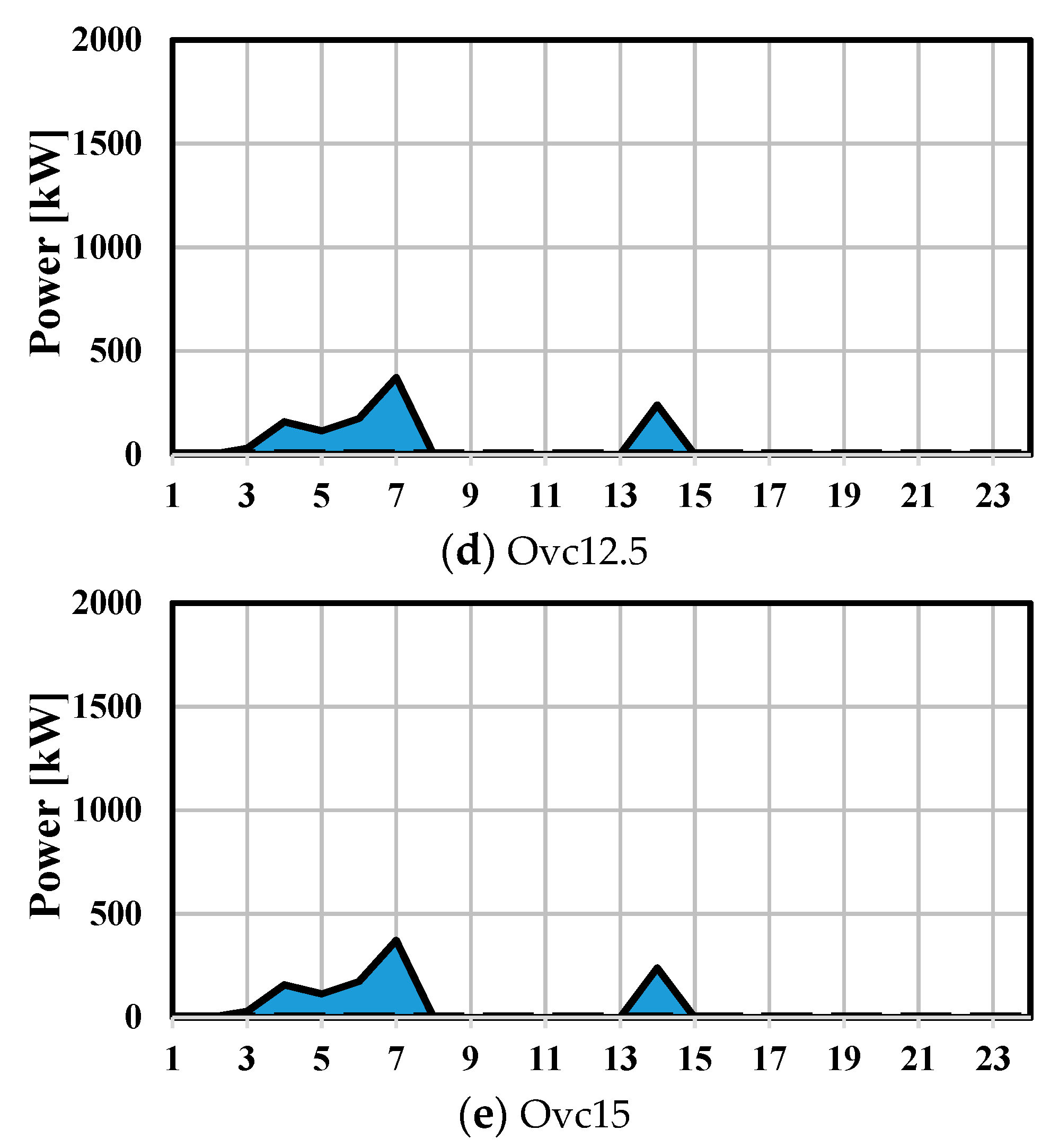
# of Transports			3	3	2	0	0

presents the result of the simulations for the Ovc case. In the table, the Ovc5, Ovc7.5, Ovc10, Ovc12.5, and Ovc15 scenarios denote 5, 7.5, 10, 12.5, and 15 percent deviation permitted in the nominal bus voltage, respectively. Renewable generation is the same as the base values in Figure 2, and there are no line flow constraints. Based on the results, utilization of the MBES will result in an 18–25 percent reduction in the daily operation cost depending on the voltage limit. Only for the Ovc5 and Ovc7.5 scenarios with stringent voltage constraints, the MBES is not capable of absorbing total curtailed energy. The MBES has also experienced the highest total number of transportations for these scenarios. The curtailment mitigation level starts from 34% and 58% for these two scenarios while reaching 100% for the last three ones. It should be noted that for the two last scenarios with wider voltage bounds, Ovc12.5 and Ovc15, the same results are obtained. Additionally, the MBES performs charge and discharge actions without transportation to avoid transportation costs. This means that the MBES can be charged or discharged directly from Bus #1 without violating voltage bounds for these two scenarios. 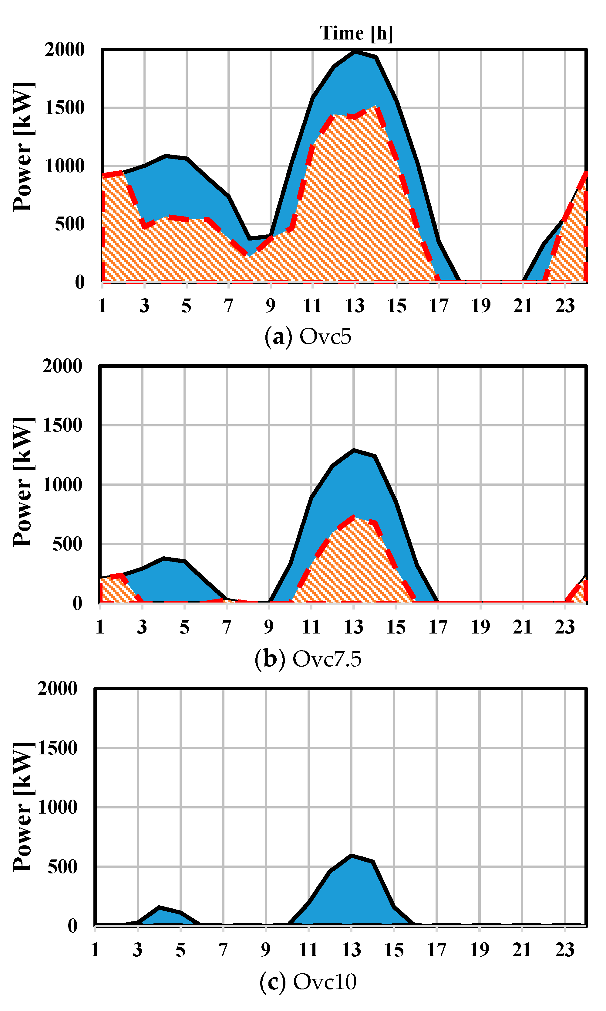Figure 4 shows hourly curtailed renewable energy for this case’s scenarios. The solid blue surface that remained behind the hatched red area denotes recovered curtailed renewable energy by the MBES. As it can be observed, the MBES is charged with the free curtailed energy at two time periods. The first one is the initial hours of the day during 3–7 a.m., with excess energy produced by the high wind speeds. The other one is from 10 to 16 when solar radiation and PV-based energy production are abundant. The MBES absorbs excess and unusable energy produced by renewable sources according to its capacity. Afterward, the stored energy is rejected back to the grid in the optimal time and location. According to the results, except for the first two scenarios where the amount of power cut is very high, the MBES performed a complete energy recovery. In other words, in the last three scenarios, the MBES fully prevented the renewable energy curtailment.

Table 6. Hourly power schedule of the MBES (kW) for Ovc case (+ Charge and − Discharge).

h	Ovc5	Ovc7.5	Ovc10	Ovc12.5	Ovc15
1	0	0	+160	+160	+160
2	0	0	+231	+231	+231
3	+247	+429	+330	+330	+330
4	+247	+464	+458	+458	+458
5	+247	+414	+414	+414	+414
6	+247	+142	0	+142	+142
7	+247	0	−229	−229	−229
8	0	−317	−617	−617	−617
9	−27	−209	−366	−494	−494
10	+247	0	−155	−155	−155
11	0	+247	+232	+232	+232
12	0	+247	+474	+474	+474
13	+247	+247	+672	+672	+672
14	0	+247	+540	+540	+540
15	+152	+247	+106	+106	+106
16	+247	0	0	0	0
17	0	0	0	0	0
18	−543	−543	−543	−243	−243
19	−650	−350	−350	−650	−650
20	−705	−675	−490	−490	−490
21	0	−330	−515	−515	−515
22	0	0	0	0	0
23	0	0	0	0	0
24	0	0	0	0	0

and

Table 7. Hourly bus location of the MBES for Ovc case (T = Transportation).

Sc.	Ovc5			Ovc7.5			Ovc10		Ovc12.5	Ovc15
Connection Bus	1	20	24	1	20	24	1	20	1	1
1
2	T			T
3
4
5
6							T
7				T
8	T
9
10–21
22				T			T
23	T
24

demonstrate the hourly power and spatio-temporal schedule of the MBES for this case. From the results, it can be observed that the battery moves to the distributed generator locations to absorb free excess energy. The MBES performs two charge/discharge cycles according to the load and the renewable curtailment pattern. In the first cycle, the MBES is transported from Bus #1 to Bus #24 to charge from the wind farm. The duration of the MBES presence at the destination bus varies according to the surplus renewable energy availability. For example, for the first scenario with the most extra energy, the MBES spends 5 h charging. This time is reduced for the other scenarios with lower extra renewable energy.

The MBES then uses the stored energy to supply the first peak load profile from 7 to 10 a.m. When it empties, it moves to the new destination where the PV panels are installed, namely Bus #20. The MBES is recharged at the bus between hours 10 and 15 according to the available excess renewable energy. The energy stored in the second cycle is finally used between 6 and 9 p.m. to supply the second load peak. At the end of the schedule, the MBES relocates to its initial location by performing the last transportation, i.e., Bus # 20 to Bus #1. In this way, the curtailed renewable energy, which has a variable temporal and spatial distribution, is collected from the network with optimal spatio-temporal and power–energy scheduling of the MBES to supply a portion of the load when needed.

Table 8. Simulation results for Olc case.

Case Title			Olc60	Olc80	Olc100	Olc120	Olc140
Total Operation Cost ($)		DN	5089	4566	4303	4059	3848
		MB	4271	3810	3575	3356	3150
		%	16.07	16.56	16.92	17.32	18.14
Curtailment (kWh)	PV	DN	8400	7335	6285	5234	4184
		MB	6161	5055	4005	2832	1782
	Wind	DN	2217	302	302	302	302
		MB	820	7	0	0	0
	Total	DN	10,617	7638	6587	5537	4486
		MB	6982	5063	4005	2832	1782
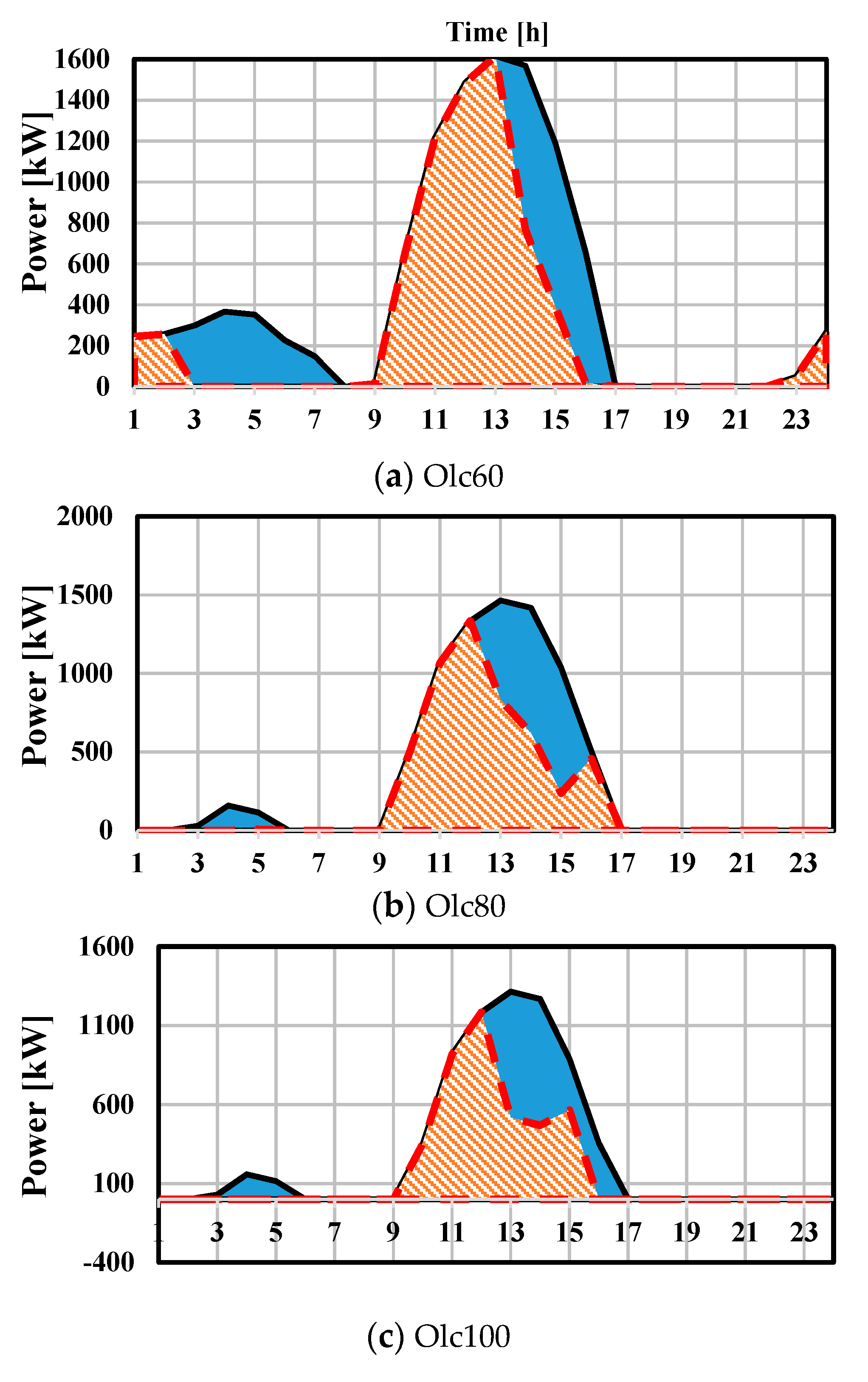
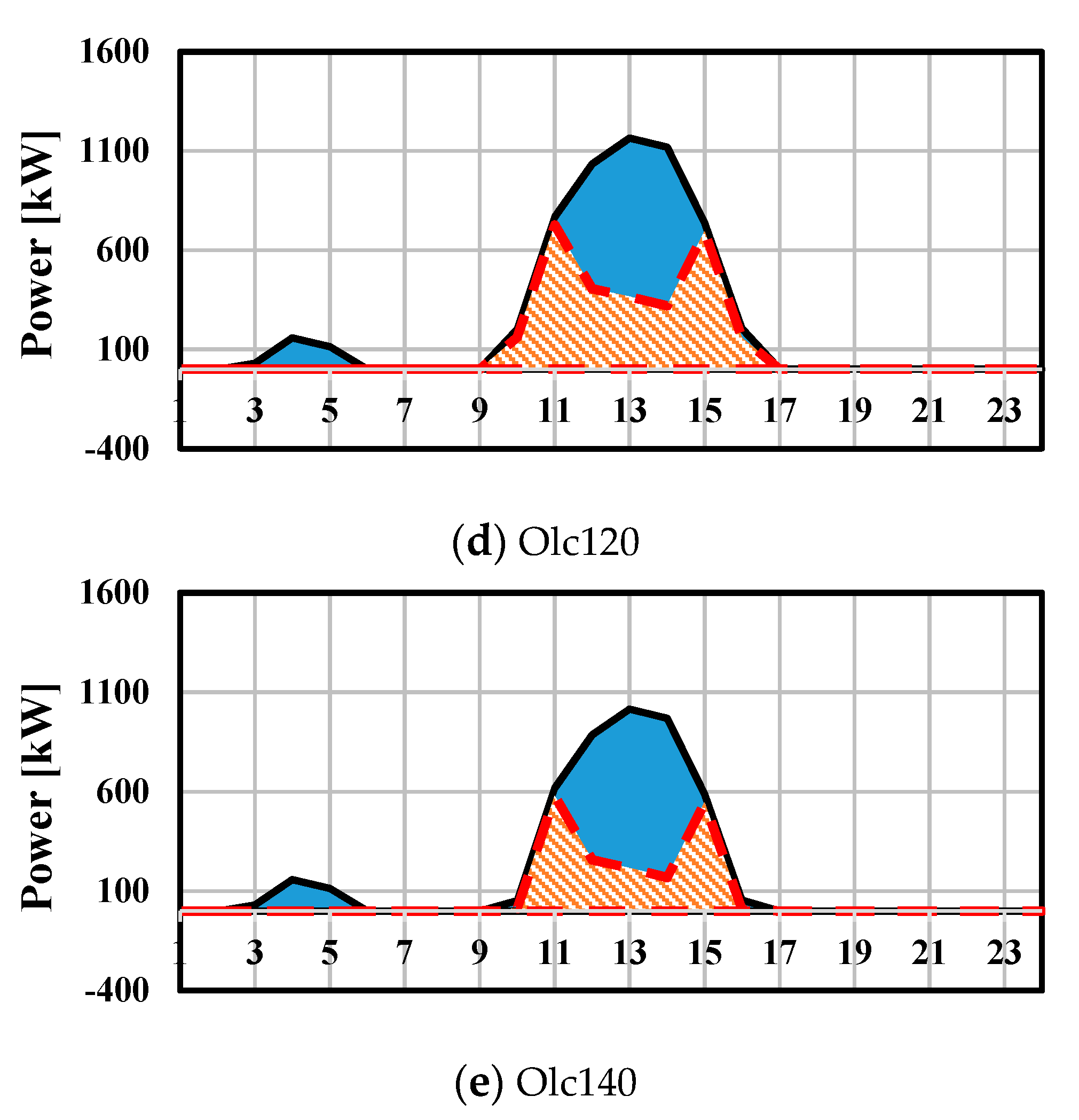
# of Transports			3	2	2	2	2

contains simulation results for the last case wherein Olc60, Olc80, Olc100, Olc120, and Olc140 scenario indicate multiplication of the capacity of the lines between buses 2–19 and 3–23 by a factor of 0.6, 0.8, 1.00, 1.20, and 1.40, respectively. Obviously, due to the limited power and energy of the MBES, it was not able to absorb all the renewable energy cut off in all scenarios. The total renewable curtailment mitigation ratio starts at about 33% for Olc60 and ends at 60% for the scenario with the lowest line congestion, namely Olc140. Moreover, the MBES’ ability to absorb excess wind energy was greater than that of the PV due to its smaller amount. The total operation cost reduction due to supplying load from the curtailed renewable energy is about 17% on average. Another point is that the MBES needs to perform at least two transports to reduce the renewable curtailment for all scenarios due to the congested lines.

Figure 5 depicts hourly curtailed wind and PV energy for this case. Besides,

Table 9. Hourly power schedule of the MBES (kW) for Olc case (+ Charge and − Discharge).

h	Olc60	Olc80	Olc100	Olc120	Olc140
1	+775	+160	+160	+30	+160
2	0	+231	+231	+231	+139
3	+630	+330	+330	+330	+330
4	+601	+450	+458	+458	+458
5	+656	+414	+414	+414	+414
6	+155	+142	+142	0	0
7	+62	0	−229	−229	−229
8	−17	−317	−317	−617	−617
9	0	−209	−209	−475	−509
10	−507	−357	−207	0	0
11	−663	−676	−604	0	0
12	−711	0	0	+587	+587
13	0	+590	+759	+759	+759
14	+758	+758	+758	+758	+758
15	+756	+756	+279	0	0
16	+590	0	+308	0	0
17	0	0	0	0	0
18	−243	−543	−543	−543	−543
19	−650	−650	−350	−650	−350
20	−490	−375	−490	−675	−490
21	−515	−330	−515	−330	−514
22	0	0	0	0	0
23	0	0	0	0	0
24	0	0	0	0	0

and

Table 10. Hourly bus location of the MBES for Olc case (T = Transportation).

Sc.	Olc60			Olc80		Olc100		Olc120		Olc140
Bus	1	20	24	1	20	1	20	1	20	1	20
1
2	T
3–5
6								T		T
7–11
12				T		T
13	T
14
15
16
17				T		T		T
18–21
22	T
23										T
24

demonstrate the hourly power and spatio-temporal schedule of the MBES for this case. Similar to the previous case and considering wind and PV location, the MBES chose Bus #24 and Bus #20 as the destinations. The MEBS transportation pattern for this case’s scenarios is quite different due to the differences in the amount and time periods of their excess renewable energy. Except for the first scenario, the MBES made only two transports. For the Olc60 scenario, considering curtailed energy on the one hand and the high line congestion, on the other hand, the MBES has decided to move to the wind park location for maximum utilization.

The stored energy at this period is used to supply a portion of the load at the first peak duration between hours 7 and 11. Subsequently, the MBES moves to Bus #20 to benefit from the free PV-based energy generation. During the second cycle, the absorbed energy is then used to meet the load demand’s second peak from 18 to 21 a.m. For the other four scenarios, the wind energy during the initial hours of the day and the less congestion in the lines is such that the battery prefers not to transport and be charged and discharged in the source bus. However, for the peak PV production hours, the MBES moves to Bus #20, considering significant excess energy. Finally, the MBES performs the second transportation, a mandatory movement to relocate to the initial location.

4. Conclusions

The MBES is a valuable asset for enhancing the distribution grids’ economic and technical performance at both emergency and normal operation states. The MBES can be used to mitigate renewable energy curtailment from wind and solar resources. Accordingly, a new MBES operation model is proposed for renewable energy curtailment mitigation. The proposed model, while considering transportation time and cost, is integrated into the distribution OPF. The case study results demonstrated that the proposed model could define the optimal spatiotemporal and power/energy status of the MBES to achieve minimum curtailment. Moreover, the MBES schedule pattern is highly dependent on the renewable energy penetration level, bus voltage limit, and congestion of the feeders. Additionally, owing to the time difference of the wind and PV maximum power generation period, the MBES can efficiently absorb excess energy by performing two cycles. The limitations of this study can constitute future research works. In line with this study, scheduling separable truck-mounted battery containers and also mobile hydrogen storage for long-term applications can be addressed. Besides, dynamic nature transportation network traffic can also be taken into account in the model.