1. Introduction
The continuously growing energy demands from depleting conventional sources and the accompanying environmental concerns with harmful green-house gas emissions and high pollution impose significant challenges to overcome. For this reason, improving energy efficiency turns out to be one of the primary objectives for academic and industrial communities to address, including the development of alternative state-of-the-art generator and low-carbon technologies. Emerging multiport electrical machines and systems [
1] are the key element in providing increased power ratings, fault-tolerant capabilities, and higher reliability relative to the existing solutions. During the past few decades, they have been rapidly developed in response to increasing requirements for a wide range of new applications such as [
1]: wind energy conversion systems (WECS), micro-grids, electric vehicles, more electric aircrafts, electric ship propulsion, high-power industrial drives, robotics, etc. Among them is certainly the Brushless Doubly Fed Reluctance Machine (BDFRM) with two electrical and one mechanical port, mostly targeting large wind generators [
2], but also commercial heating, ventilation and air conditioning (HVAC) and large pump-type drives, as well as turbo machinery [
3]. The BDFRM main advantages can be summarized as the following [
2]:
- -
Maintenance-free operation due to robust structure (no brushes and slip rings) and high reliability unlike the traditional Doubly Fed Induction Machine (DFIM);
- -
Inherently medium-speed operation allowing the use of a two-stage gearbox, instead of a vulnerable three-stage counterpart with DFIMs, offering greater mechanical robustness and lower failure rates, hence the apparent cost benefits;
- -
A small-capacity power-electronics converter (approximately 25–30% of the machine rating) for a typical speed range of 2:1 in wind turbines and pump drives;
- -
Superior low-voltage-fault-ride-through (LVFRT) and grid integration properties to DFIG afforded by the relatively large leakage inductances and lower fault current levels allowing simpler protection of the partially-rated converter, often without a crowbar circuitry [
4];
- -
Operating mode flexibility as it can operate as a classical IM (which is an important ‘fail-safe’ feature in case of the inverter failure), or as a fixed/adjustable speed synchronous turbo-machine, enabling high-speed, field-weakened traction applications, as well as high-frequency generators [
5].
The drawbacks that may be associated with the BDFRM are compromised torque density [
3], efficiency, and power factor [
2]. In order to minimize these limitations and enhance its market competitiveness, further performance improvements are necessary, especially through the rotor optimization [
2]. This promising machine technology is still evolving and according to the latest design and control advances it should be seriously considered as a viable substitute to DFIMs, foremost as a wind turbine generator (BDFRG) [
3]. The BDFRMs have therefore gained increasing attention given their numerous advantages not only over DFIMs, but also its Brushless Doubly-Fed Induction Machine (BDFIM) counterpart, which is much more difficult to control due to the heavy parameter dependence of dynamic models [
6].
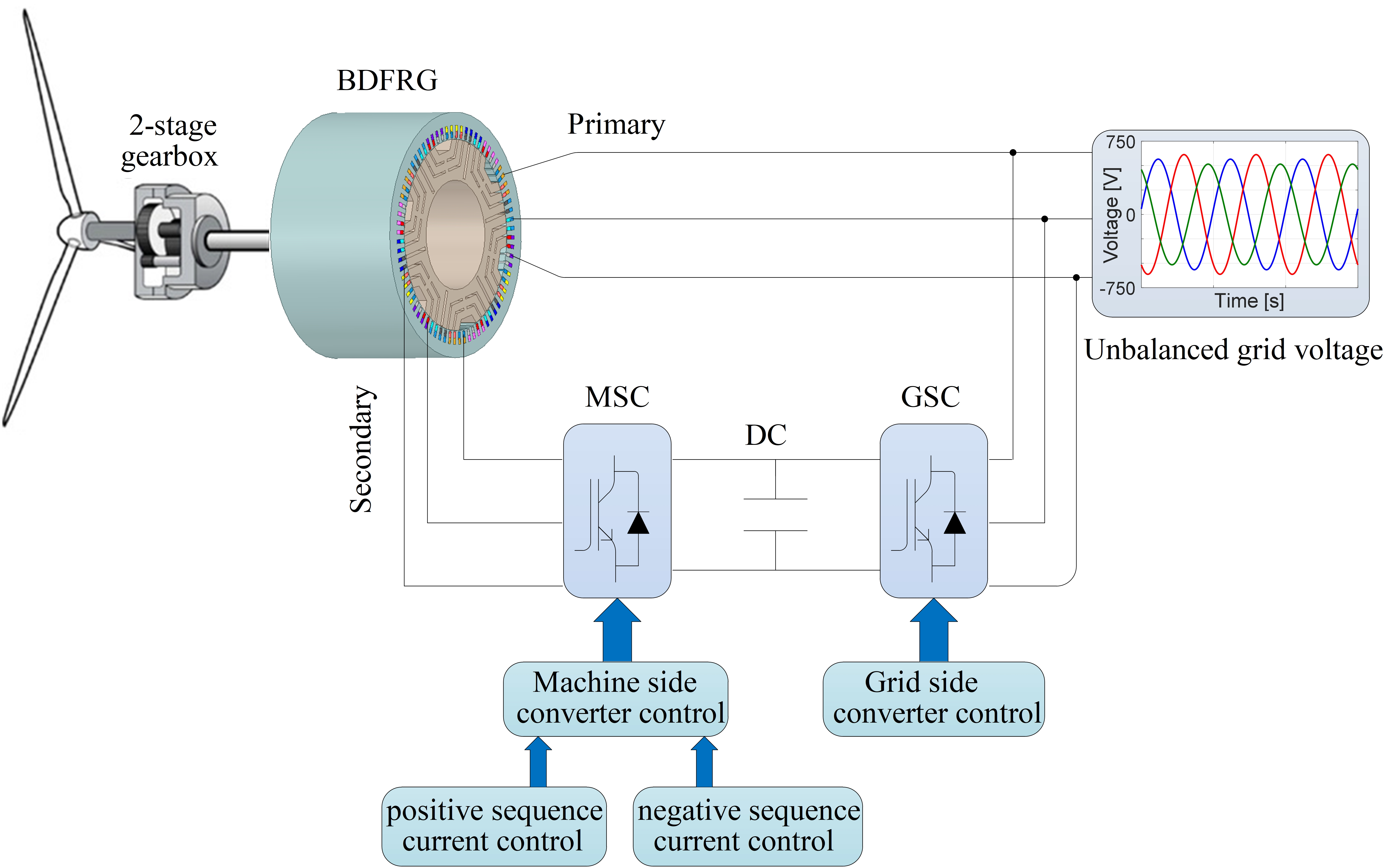
The BDFRM is a self-cascaded, slip power recovery machine [
3] with two conventional, sinusoidal stator windings of different applied frequencies and pole numbers [
7], and a modern reluctance rotor having half the total number of stator poles to provide magnetic coupling between the windings. Thus, a pre-requisite for the torque production is established by modulating the stator magneto-motive force waveforms and generating flux through a variable air gap. The primary (power) winding is directly connected to the grid, while the secondary (control) winding is usually fed by a bi-directional power converter with variable voltage and frequency to allow the super or sub-synchronous speed variations in either operating regime, i.e., as a generator (BDFRG) or a motor (
Figure 1). If the angular frequency and the number of pole pairs of the primary winding are
ωp and
Pp respectively, and those of the secondary winding are
ωs and
Ps, than the BDFRM ’natural’ synchronous speed (i.e., with the DC secondary,
ωs = 0) is
ωsyn =
ωp/Pr, where
Pr is the number of rotor poles, i.e.,
Pp +
Ps. The machine operation is determined by the power flow through the primary side, i.e., from the grid for the motor (i.e., torque
Te > 0), and to the grid for the BDFRG (
Te < 0), while the secondary winding can consume or deliver active power subject to the phase sequence, i.e., the
ωs sign: the BDFRM would absorb (produce) positive power via the secondary at super (sub)-synchronous speeds as a motor, and at sub (super)-synchronous speeds as a generator.
Regarding the WECS, various control principles to extract maximum power from the wind turbine have been reported in the literature over the years. They can be mainly classified as scalar control [
5,
8,
9,
10], vector control, which can be voltage oriented control (VOC) or field-oriented control (FOC) [
4,
11,
12], and direct torque control [
5,
13,
14]. These control techniques can be shaft position sensor based or sensorless [
15], established through different position or speed estimation methods, including Model Reference Adaptive System (MRAS) [
12,
16] or observer-based schemes for speed, as well as torque (and flux) control [
17]. The underlying control strategies have different objectives such as: power-winding unity power factor [
11,
18], minimum converter current or maximum torque per inverter ampere (MTPIA), minimum copper losses, maximum power factor [
11], reactive power and torque control [
19], or Direct Power Control (DPC) [
20,
21,
22,
23]. Besides, other approaches such as Open-Winding-Based control [
24,
25], improved Particle Swarm Optimization to adequately track the speed [
26], and etc. have also been documented.
All of the previous methods are concerned with the balanced operating conditions of the BDFRM. There are two main reasons to consider dynamic modeling and control aspects under unbalanced voltage conditions. Firstly, wind turbines are often installed in remote areas with weak grids where unbalanced voltages are common [
27]. Secondly, the power system’s transient stability issues with high penetration of WECS in recent years and consequently their large impact on the electricity system steady-state and dynamic operation [
28,
29]. Therefore, under voltage dip conditions caused by faults within the grid, wind generators have to stay connected and act similarly to conventional power plants providing active power control, frequency regulation, and dynamic voltage control, as well as low voltage ride through (LVRT) [
28,
29]. These requirements are specified by transmission system operators as grid codes for different countries and regions.
Under unbalanced conditions, negative-sequence components are present in the grid voltage, causing problems for wind generators such as unbalanced primary currents, current harmonics at the secondary side, unequal heating, or hot spots in the windings [
30] which degrade the insulation and reduce the life expectancy of the windings, as well as producing power pulsations [
31,
32]. Unbalanced currents also create a pulsating torque, which may cause extra mechanical stress on the drive train and gearbox [
33,
34,
35,
36] and increase acoustic noise, too. Therefore, studying wind generators under unbalanced grid voltage conditions and designing a convenient control strategy are very important.
A new model for the BDFRG unbalanced operation was put forward in [
34] using positive and negative sequence equations. The same authors used the model presented in [
34] to develop a Predictive DPC (PDPC) method for the BDFRG under unbalanced grid conditions in [
30]. The proposed PDPC is based on a power compensation strategy aiming to achieve two control objectives: balancing the primary currents and mitigating the electro-magnetic torque pulsations. However, the impact of unbalanced grid voltage on the primary active power and the secondary current has not been fully investigated. To the best of the authors’ knowledge, there is no other work on vector control under unbalanced grid conditions in the BDFRG (M) literature to date either.
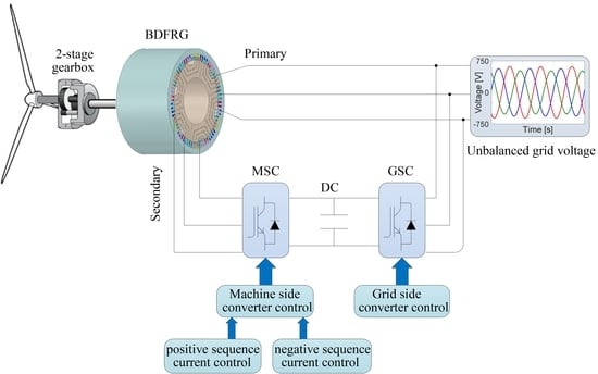
This paper aimed to partly fill the existing void by presenting the main concepts, design aspects, and simulation verification of the advanced vector control strategy developed for unbalanced grid voltage conditions with the intention to simultaneously achieve the primary active power and the secondary current control. A modified vector control scheme was proposed for the BDFRG to control the positive and negative sequences of the secondary currents independently. In the primary flux-oriented positive and negative (dq) reference frames, the model of the BDFRG with unbalanced terminal voltages was developed and subsequently used to derive the control form relationships between torque and active and reactive power, including positive and negative components.
The paper is organized as follows: after the Introduction, the dynamic model of the machine under balanced conditions is presented in
Section 2. The BDFRM mathematical model for unbalanced grid voltages is presented and discussed in
Section 3.
Section 4 describes the system behavior with conventional vector control under unbalanced conditions. An improved vector control design is presented to address the negative sequence components in
Section 5, where the corresponding current references are calculated for different control targets. The improved control is verified by computer simulations in
Section 6, demonstrating the potential of the proposed control strategy. Finally, the main results are summarized in the Conclusions.
2. BDFRM Model under Balanced Conditions
The BDFRM(G) space vector dynamic model in rotating
dq reference frames assuming
motoring convention can be represented as in [
37]:
where
up and
us are the primary and secondary winding voltages respectively, while
λp and
λs are the corresponding fluxes. The remaining parameters are as follows: the primary and secondary winding resistances
Rp and
Rs, and self-inductances
Lp and
Ls,
Lps is the primary to secondary mutual (magnetizing) inductance,
σ = 1–
L2ps/(
LpLs) is the leakage factor,
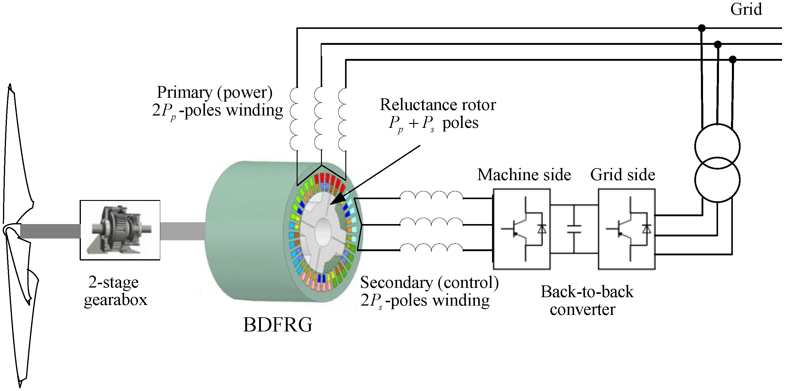
λps is the mutual flux linkage, and “*” denotes a complex conjugate as usual. All the vectors in the primary voltage and flux equations are stationary in a
dq reference frame rotating at
ωp, and so are secondary counterparts but in a
ωs rotating
dq reference frame shown in the phasor diagram of
Figure 2. Note that
ism =
is and
ipm =
ip (in their respective frames) are the magnetically coupled currents from one machine side to the other, with the same magnitude albeit a different frequency to the originating current vectors as a result of the frequency modulating action of the rotor [
7,
37].
The fundamental relation between the angular frequency of the primary (
ωp), the angular frequency of the secondary (
ωs), and the electrical angular velocity of the rotor (
ωr) can be written as,
where
ωrm is rotor mechanical angular velocity.
Active and reactive power of the primary winding are expressed as follows
where the electromagnetic torque expression using the primary quantities is:
The dynamic performance of the BDFRM(G) connected to the grid with balanced voltages is completely characterized by (1)–(5).
3. Mathematical Model under Unbalanced Grid Voltage Condition
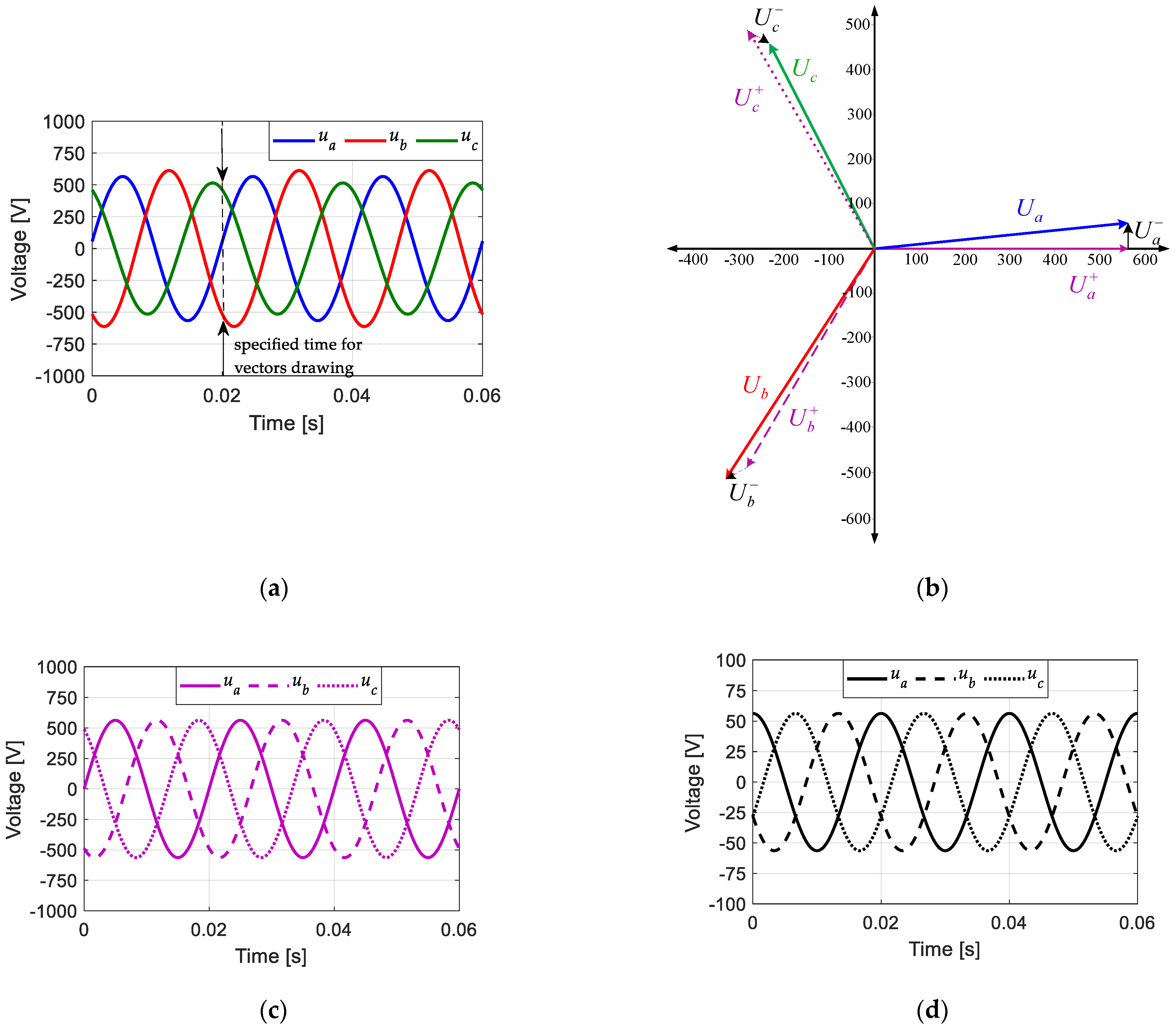
Each unbalanced three-phase system can be divided into three balanced three-phase systems using the symmetrical component theory, i.e., positive, negative, and zero sequence. Assuming no zero components (because of the isolated neutral), any vector can be decomposed into symmetrical positive and negative sequence components [
38]. Therefore, unbalanced voltages of a weak grid can be described as the sum of the positive and negative sequences as shown in
Figure 3.
In case of unbalanced grid voltages, all primary variables (voltages, currents, and fluxes) can be expressed in a stationary (αβ) reference frame as follows:
where
Fp1 and
Fp2 are the modules of the positive and negative sequences respectively, while
φ+Fp and
φ−Fp are their initial angular positions. Transforming (6) into the primary reference frame (by multiplying with
e−jωpt) leads to (7):
where
F+p and
F−p are the positive and negative sequence components of
Fp in the respective positive and negative reference frames rotating at
ωp and −
ωp, respectively.
Likewise, any secondary winding variable represented in the space vector form in the αβ frame under unbalanced grid voltage conditions can be expressed as:
where
Fs1 and
Fs2 are the modules of the positive and negative sequences, respectively, and
φ+Fs and
φ−Fs are their initial angular positions. By multiplying (8) with
e−jωst one obtains:
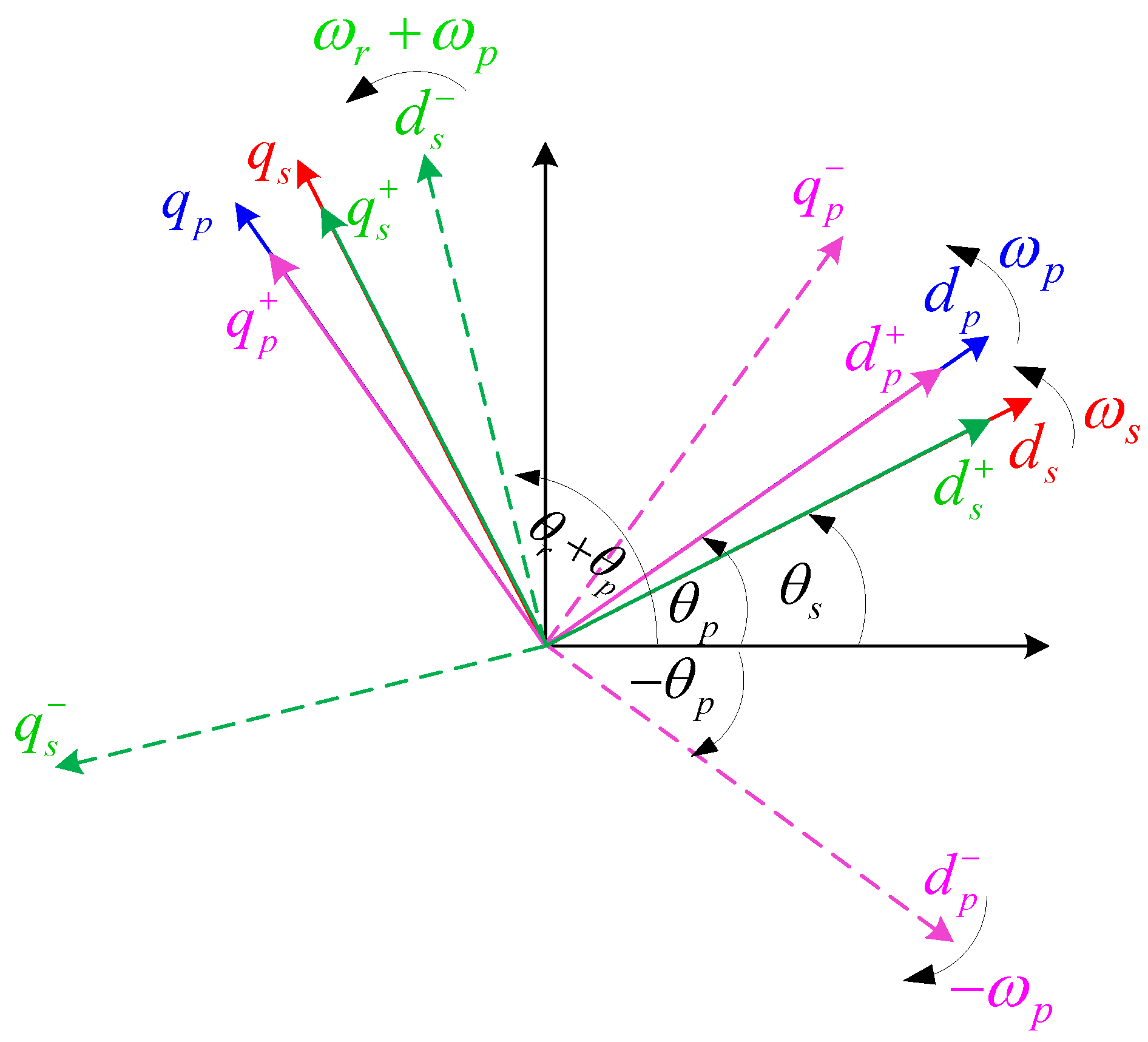
where
F+s and
F−s are the positive and negative sequence components in the respective positive and negative reference frames rotating at (
ωr −
ωp) and (
ωr +
ωp), respectively. The reference frames of the BDFRG unbalanced model are illustrated in
Figure 4.
The space vector model of the BDFRG using the positive and negative sequences can be obtained by substituting (7) and (9) into (1) and (2) [
34]:
It is worth noting that the positive sequence equations are similar to the space vector model under balanced conditions given by (1) and (2). The negative sequence model can be obtained in a similar manner [
34]:
Using the aforementioned space vector equations, one can now derive the
dq equations for the positive and negative sequences as follows,
where the fluxes are:
Similarly, for the negative sequence, the
dq equations are:
and
3.1. Power and Torque Relationships
The power and torque expressions can be derived by substituting the
dq positive and negative components into (4) as [
34,
39]:
It can be observed from (25) and (26) that there are DC components Pp0 and Qp0, together with the oscillating terms at double supply frequency, pp-sin, pp-cos and pp-sin, pp-cos, which indicate the presence of negative sequence components.
An average (DC) value and two components oscillating at 2
ωp also constitute the secondary active and reactive power given the following:
The electromagnetic torque expression for the BDFRG under unbalanced conditions can be obtained by substituting (7) and
F =
Fd +
jFq into (6):
Therefore, apart from the fundamental component Te0, there are two additional oscillating terms at 2ωp. Therefore, we can conclude that unbalanced grid voltages cause the appearance of pulsations in the power and torque waveforms.
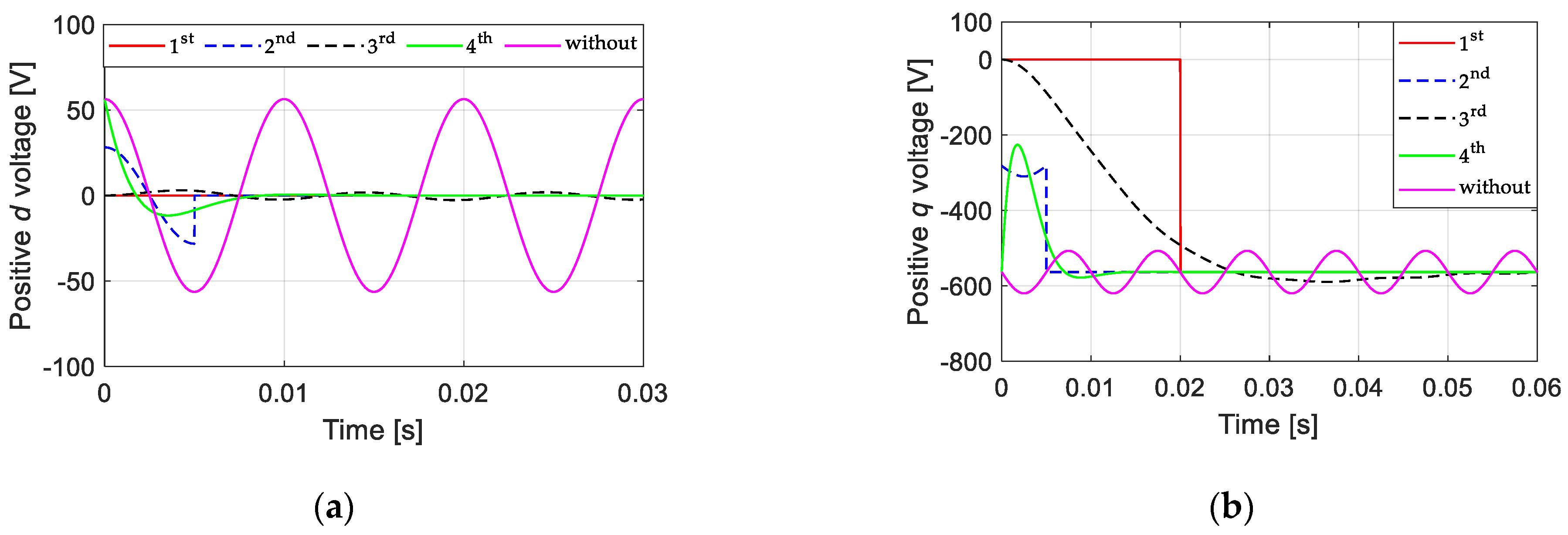
3.2. Methods for Real-Time Separation of Positive and Negative Sequences
The effectiveness of the proposed control method highly relies on the accurate separation of positive and negative sequences in real-time. There are mainly four methods reported in the literature: the analytically based method [
34], “Signal delay cancellation” [
40], and filtering methods, i.e., low-pass filters [
40] and notch filters (band trap, band-stop) [
41]. Any of the listed methods reported in the literature can be used for this purpose.
The first method, which is the analytically based method presented in [
34], is derived from the fact that
F+pd,
F+pq and
F+sd,
F+sq represent the DC components of
Fpd,
Fpq,
Fsd and
Fsq because frequencies of
F+p and
F+s are respectively equal with the frequencies of
dqp and
dqs frames. In other words,
F+pd,
F+pq and
F+sd,
F+sq are the mean values of
Fpd,
Fpq,
Fsd, and
Fsq.
The real and imaginary part of (7) and (9) can be expressed as,
where
,
,
and
are the mean values of
Fpd,
Fpq,
Fsd, and
Fsq, respectively. Therefore, the negative sequence components can be obtained from (30) and (31) as:
“Signal delay cancellation” is the second method, which is described in [
40]. The
abc system is firstly converted to the stationary
αβ reference frame using Clark’s transformation, and then delayed for T/4 as formulated below:
The signals generated in this manner are further processed to separate positive and negative sequence components as follows [
40]:
Furthermore, the
dq positive and negative sequence components can be calculated as:
Finally, with the third method described in [
40] and the fourth method described in [
41], the positive (negative) Park’s transformation is applied to variables
F in the
abc system to produce variables
F in the positive (negative)
dq synchronously rotating reference frame. It is well known fact that negative sequence components manifest themselves as second-order harmonics in the positive
dq synchronously rotating reference frame according to (7), and vice-versa for the positive sequence components. Hence, a low-pass filter [
40] or notch filter [
41] can be used to separate positive and negative sequence components in real time.
Without the aforementioned separation methods, the unbalanced three-phase voltages or currents have second-order harmonics in the
dq positive synchronously rotating reference frame as shown in
Figure 5. This figure also presents the results of applying the four listed separation methods. The separation of positive and negative sequences must be accurate, fast, and with as low oscillations as possible at the beginning and at the end of voltage dip. Based on results presented in
Figure 5 and according to chosen criteria, the “Signal delay cancellation”, or the second separation approach offering the best transient performance was adopted in the generator model under unbalanced conditions presented in this paper. For the control system, notch filter presented as the fourth method was chosen, which has a slightly worse performance, but simpler implementation.
4. Conventional Vector Control
Using the BDFRG model for balanced conditions given in
Section 2, the following important power relations for the primary voltage vector-oriented control (VOC) and flux-oriented control (FOC) can be derived [
4]:
By observing the VOC expressions, there are coupling terms since
isd and
isq appear in both real and reactive power relationships of (41). The level of coupling can be reduced by aligning the
qp-axis to the primary voltage vector (
Figure 2). If the
dp-axis is aligned to the primary flux linkage (i.e.,
λpq = 0), the primary flux-oriented control (FOC) is realized [
15]. The most important advantage of FOC over VOC is the inherently decoupled control of the primary active and reactive power. However, these appealing FOC properties come at the cost of the primary flux angle estimation. In addition, the primary winding resistance may need to be known in low to medium-power applications [
14].
From
Figure 2 it can be seen that if the
dp-axis lies along the
λp, the
ds-axis of the secondary (control) frame will align to
λps. Under this condition, the primary active power depends upon the
q-axis current component of the secondary windings. Furthermore, reactive power depends upon the
d-axis current component of the secondary windings as clearly illustrated in (42). Consequently, this enables the decoupled control of active and reactive powers. However, primary-FOC requires the estimation of primary flux angle, which, in turn, depends on the primary winding resistance (
Rp). The effect of primary resistance is small with larger machines having lower resistances.
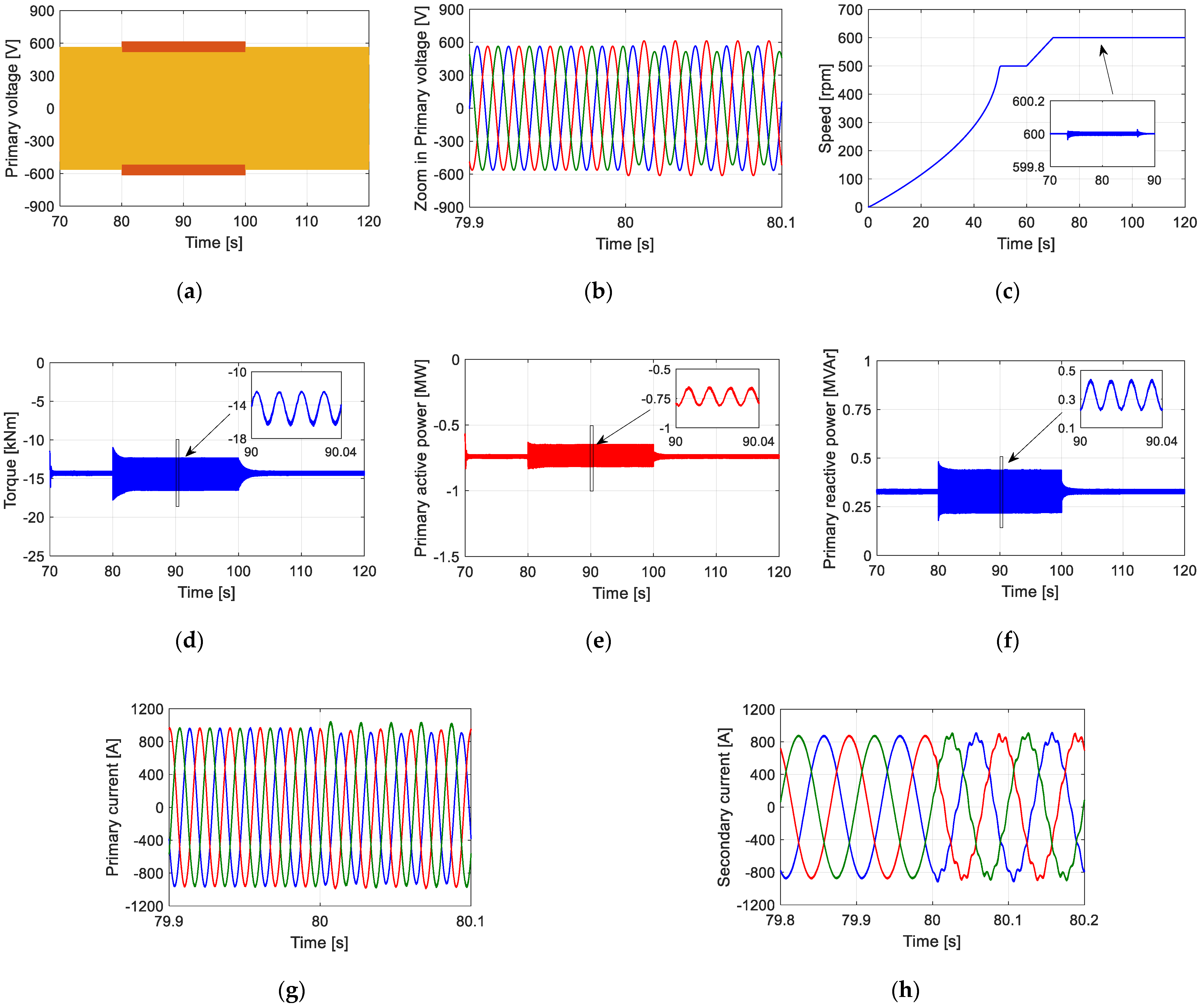
In order to demonstrate performance of the conventional vector control under unbalanced grid conditions, simulations on the dynamical model were conducted. The following test was performed: after starting the machine as a slip-ring-induction machine (i.e., with the shorted secondary winding) and achieving synchronous speed, the reference speed of 600 rmp in super-synchronous generator mode was required. After reaching a steady state, 10% VUF was introduced at 80 s and terminated at 100 s. The system response for the conventional single
PI current control design to a given period of unbalanced operation is shown in
Figure 6. The maximum torque per inverter ampere (MTPIA) objective was selected by adopting
isd = 0. This approach allowed for the minimization of the
is magnitude, and hence the reduction of both the copper and converter losses, for a given torque. Although the averaged active and reactive powers were regulated, significant power oscillations were observed due to the sine and cosine terms in (25) and (26).
With the conventional single
PI secondary current controller, the primary current became unbalanced in the presence of grid voltage unbalance (
Figure 6g). The secondary currents, whose angular frequency can be calculated from (3), contain both the fundamental component of 10 Hz and the harmonic component of 110 Hz as in
Figure 6h. The measured primary current unbalance, i.e., the deviation from the positive value was about 5.2% and a total harmonic distortion (THD) of the secondary current was about 3.7%. In addition, all the time functions of the primary active and reactive power, and the electromagnetic torque, contained significant 100 Hz pulsations, which were about 14%, 27.4%, and 11.5% of the average value, respectively.
One can conclude that, during grid voltage unbalance, the positive sequence components are well regulated by common PI controllers, while the negative sequence component rotating at double grid frequency cannot be regulated due to the controller’s limited bandwidth. Therefore, conventional vector control without backward sequence control is not able to solve the problems associated with the unbalanced grid voltage effects and consequently yields an unsatisfactory performance.
5. Proposed Control Strategy under Unbalanced Grid Voltage Conditions
Under unbalanced conditions, the positive and negative sequence components were completely decoupled as shown in (18)–(24), and thus the BDFRG can be controlled in
dq positive and negative reference frames independently. There are four secondary current components, i.e.,
i+sd,
i+sq,
i−sd, and
i−sq to be controlled. Apart from the average primary active and reactive power, i.e.,
Pp0, and
Qp0 in (25) and (26), two more parameters can be controlled. Hence, there are four selectable control targets that can be addressed [
41]. Using the FOC approach by aligning the
d+p -axis to
λp, i.e.,
λ+pq = 0, the secondary reference current can then be calculated for each selectable control target, as further elaborated.
The balanced primary currents imply that
i−pd = 0 and
i−pq = 0. According to (23), the primary negative sequence currents are given as:
Thus, the reference negative sequence secondary currents can be defined as:
Therefore, the converter intentionally injects the backward sequence currents into the secondary winding to suppress the corresponding components in the primary [
39].
In this case, there will be no double-frequency power oscillations appearing in the primary active power. Considering
λ+pq= 0, the oscillating terms of the primary active power in (25) should be zero i.e.,
pp_cos =
pp_sin = 0. This can only be achieved under the following conditions:
According to (23), the reference negative sequence secondary currents for control purposes can then be expressed as follows:
For this target, the pulsating terms of the electromagnetic torque shown in (29) have to be eliminated, i.e.,
Te_cos =
Te_sin = 0. This condition can only be achieved if the BDFRG is controlled with the reference currents formulated as:
In this case, the converter control attempts to eliminate the negative sequence of the secondary currents. The most straight-forward approach of mitigating the secondary current oscillations is setting the negative sequence secondary current references to zero,
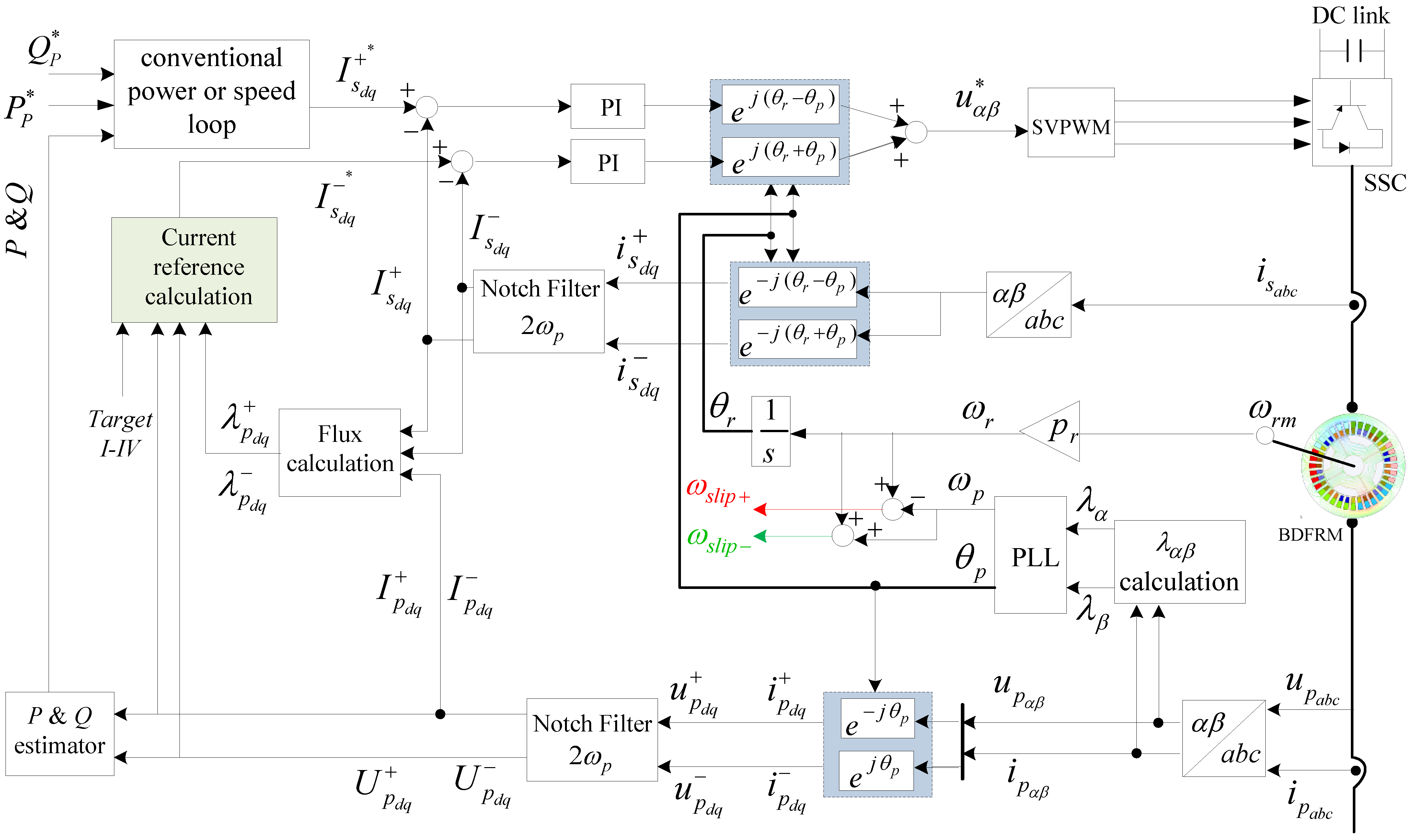
In order to implement the aforementioned control strategies, a new control algorithm was proposed as shown in
Figure 7.
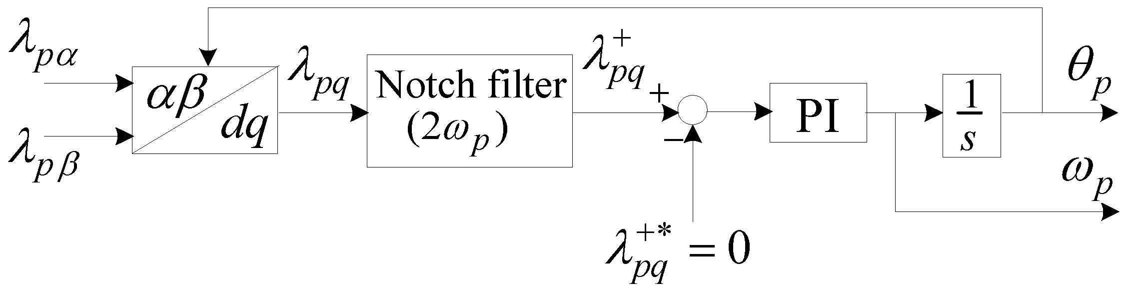
Under unbalanced conditions, the primary flux contains both positive and negative sequence components. Its stationary frame components can be estimated as:
To achieve an accurate reference frame transformation, the PLL must only recognize the positive sequence primary flux [
42]. Therefore, a notch filter was applied and tuned at twice the line frequency to remove the negative sequence components (
Figure 8).
Once the angular velocity ωp and position θp of the positive sequence primary flux are detected by the PLL, primary currents and flux in the stationary αβ frame can be transformed to dq+p and dq−p rotating reference frames. Likewise, the secondary current can be transformed to dq+s and dq−s reference frames.
In the
dq+ reference frame, the positive sequence components appear as DC and the negative sequence ones are oscillating at 2
ωp, and vice versa in the
dq−. Thus, to separate the positive and negative sequence components, notch filters tuned at 2
ωp were used in the respective reference frames to remove the oscillating terms as illustrated in
Figure 7.
6. Simulation Studies
The simulations of the proposed control algorithm were carried out in
Matlab/Simulink using the parameters of a 1.5 MW BDFRG-based WECS provided in
Appendix A. The rated DC-link voltage was set to 1200 V and a standard Space Vector Modulation (SVM) with a switching frequency of 4 kHz was used. The Maximum Torque Per Inverter Ampere (MTPIA) strategy [
43] was implemented in
Figure 7 for the main controller, by setting
i+sd = 0. The simulated turbine was assumed to have a torque-speed profile as follows [
44],
where
nr and
Tr are the rated speed and torque respectively,
nrm is the BDFRG speed.
Under regular grid conditions with negligible voltage imbalance, the system is regulated with a conventional controller, while the auxiliary one (i.e., negative sequence current controller) is disabled. When the voltage unbalance is detected, the latter is instantly enabled and the negative sequence reference currents are generated subject to the selected control target. The positive and negative sequence reference currents are passed to the main and auxiliary PI controller to produce the required secondary control voltage.
Initially, the system runs under balanced conditions with the BDFRG being started as a slip ring induction machine (i.e., with the shorted secondary winding). After reaching the steady-state, the conventional FOC is enabled, and a 10% voltage unbalance instigated at 80 s time instant.
Figure 9,
Figure 10,
Figure 11 and
Figure 12 show a comparison of the responses obtained by conventional vector control and the proposed control design in different modes. The difference between the control modes is a consequence of different target selection.
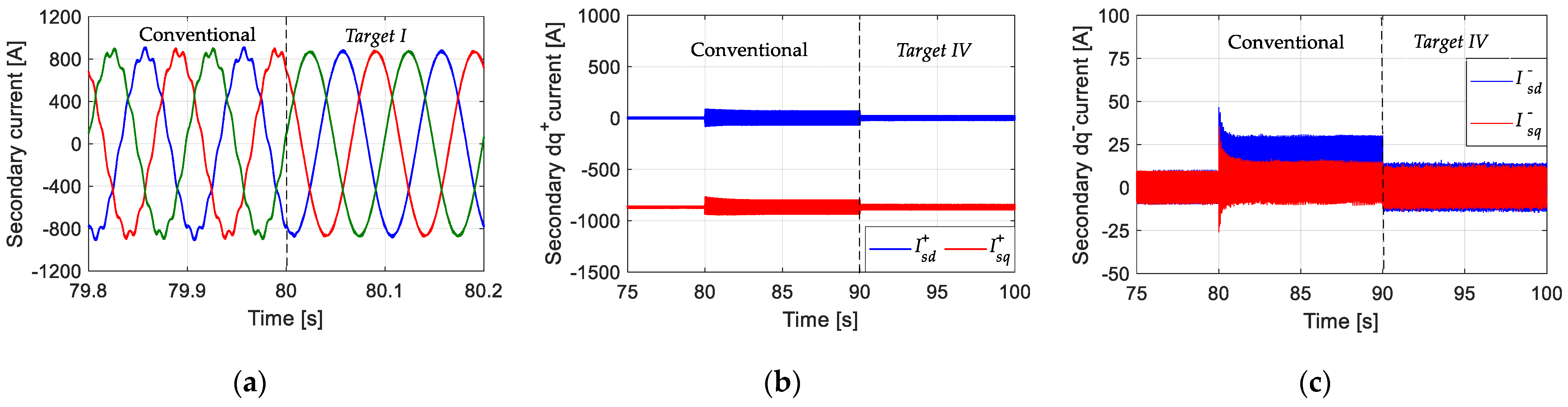
Following the unbalance inception at 80 s, the conventional design cannot provide adequate control of the negative-sequence currents, resulting in significant active power oscillations and unbalanced currents in the primary winding. On the contrary, with the proposed control design, the negative sequence currents were completely controlled according to the
Target I requirements as illustrated in
Figure 9.
It can also be seen that with the proposed controller, the operation of the system was much smoother with reduced primary active power pulsations according to the
Target II requirements as shown in
Figure 10.
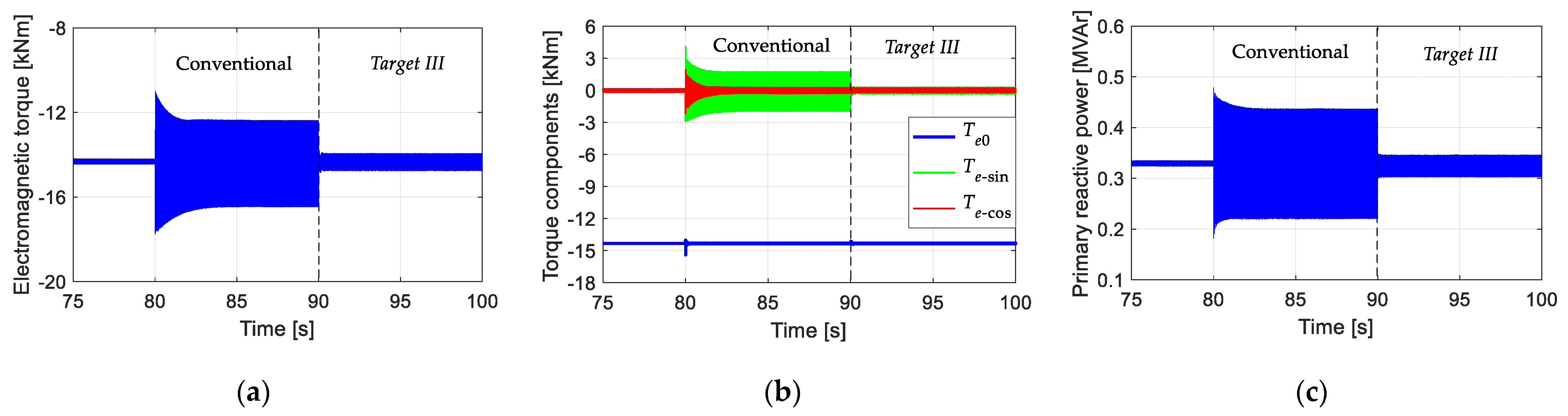
Figure 11 shows that the proposed control design with
Target III can improve the BDFRG generation system during the voltage unbalance period by eliminating the torque oscillations, which are the most concerning issue during grid voltage unbalance [
41]. According to (26) and (29), the primary reactive power pulsations are also suppressed.
Under unbalanced conditions, the secondary current contains both the 10 Hz fundamental component (positive slip 60–50 Hz) and the 110 Hz harmonic component (negative slip 60 Hz + 50 Hz), which can be eradicated by applying the proposed control with
Target IV. Hence, the secondary current immediately became harmonic free as it is clearly observed from
Figure 12.
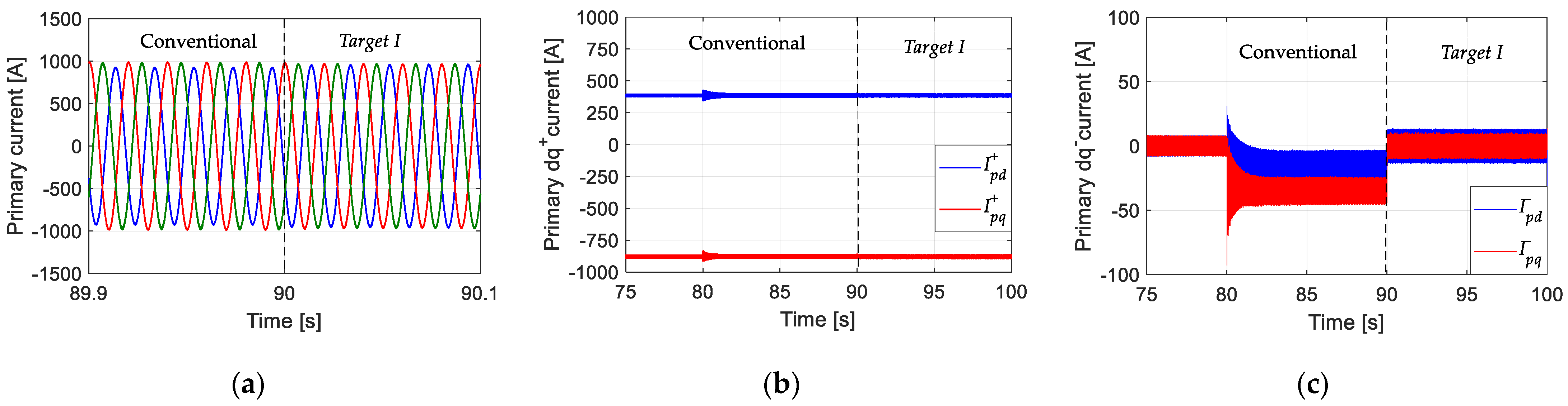
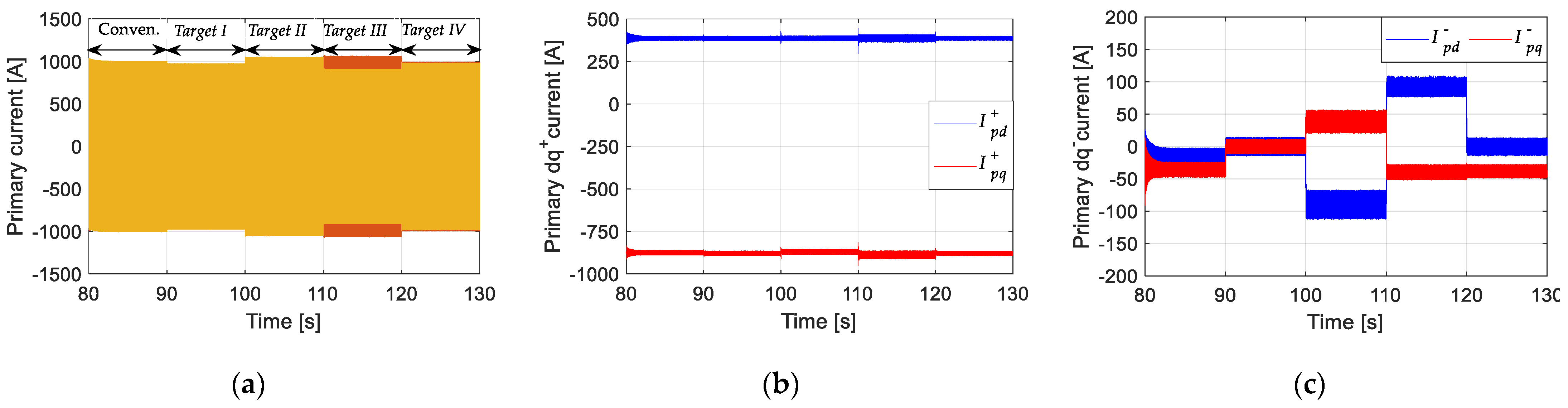
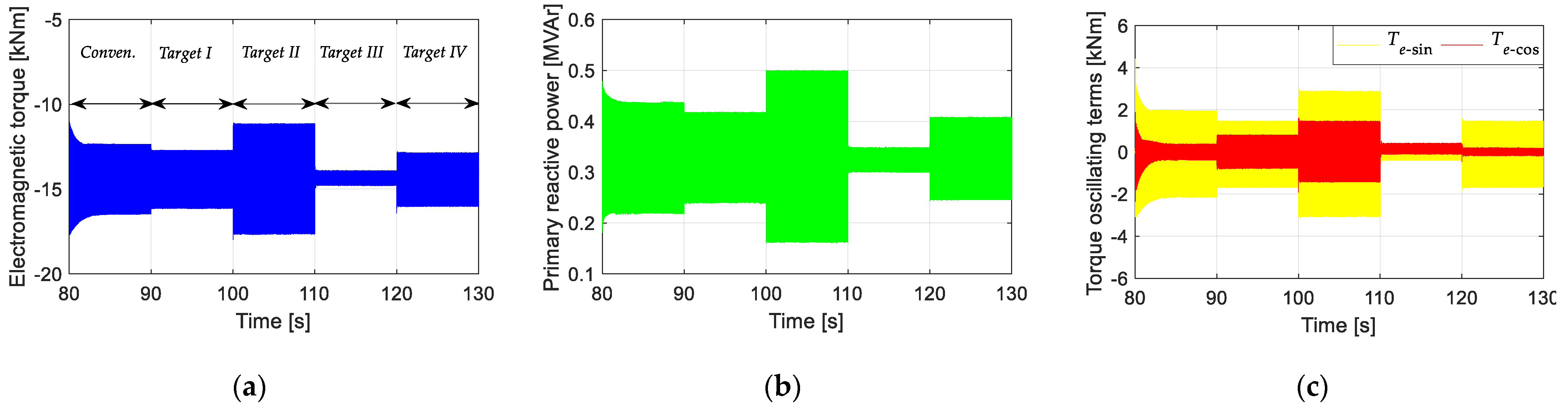
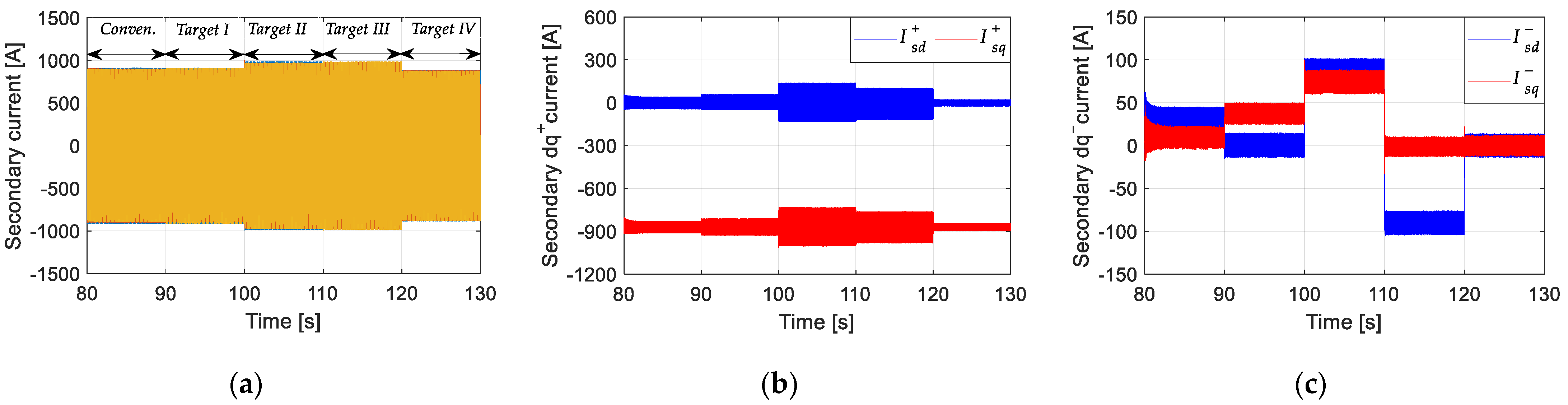
In order to assess the control targets under consideration, they were applied sequentially with a 10% voltage unbalance factor as shown in
Figure 13a. For all four control objectives,
Pp0 and
Qp0 were controlled to be constant. As a result, the positive sequence components,
i+pdq and
i+sdq remained constant, too. With
Target I,
i−pdq was controlled at zero.
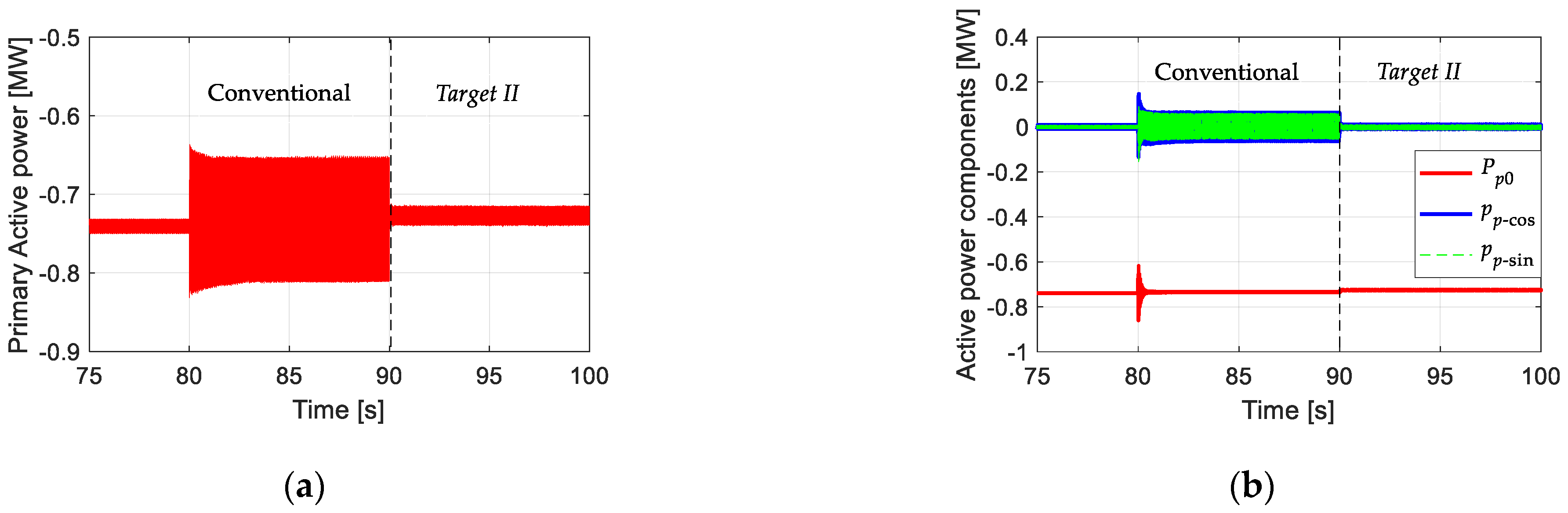
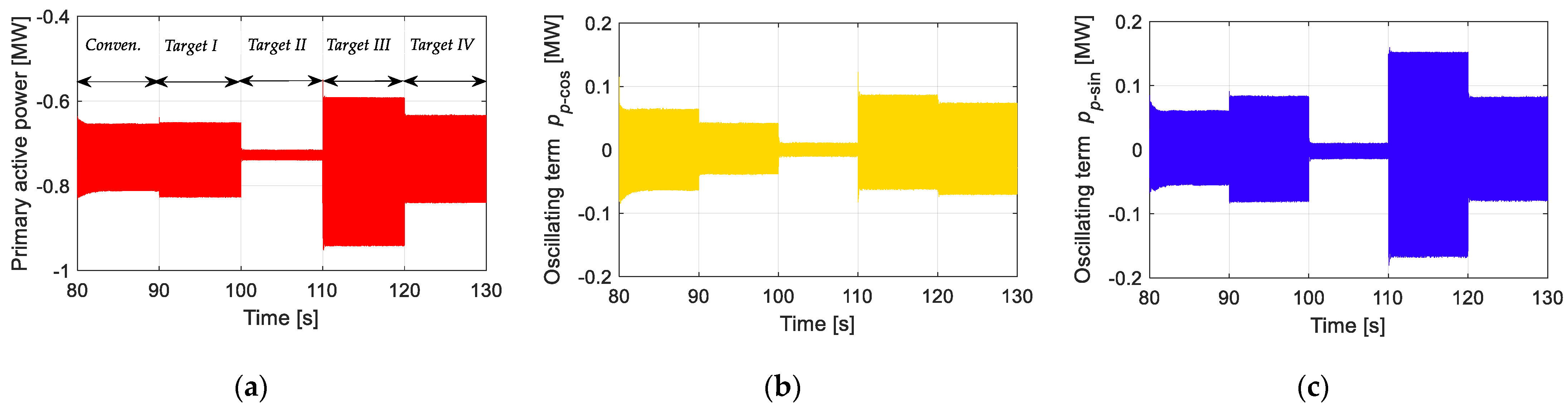
With
Target II, further reduction of active power oscillations was achieved as shown in
Figure 14. Although, in principle, the oscillations should be fully removed, this was not accomplished due to 2
ωp harmonic effects. This phenomenon has also been reported with DFIGs, and BDFIGs and they have been attributed to converter influences [
39].
Figure 15 shows that by applying the proposed control strategy with the
Target III, the BDFRG generation system during voltage unbalance can be improved by eliminating the double-frequency pulsations of electromagnetic torque. It can be also observed that the pulsation of primary reactive power is diminished as expected from (26) and (29).
With the
Target IV, the negative sequence components were completely eliminated as shown in
Figure 16. Furthermore, performance improvements in primary current, torque, and reactive power can also be seen in
Figure 13 and
Figure 15, as well as in
Table 1.
For different control targets,
Table 1 summarizes the following metrics: the primary currents unbalance, relative amplitude of the 11th harmonic (110 Hz) to the fundamental component (10 Hz) of the secondary current (
Is distortion), pulsations of the generator torque, and pulsations of the primary active and reactive power.
As can be seen from
Figure 13,
Figure 14,
Figure 15 and
Figure 16 and
Table 1, with the controller set to
Target I, the primary current unbalance became very low (about 1.2%) compared with 5.2% with conventional design. When it is switched to
Target II at 100 s, the primary active power pulsations were reduced to 2.6%. When
Target III was chosen at 110 s, the torque pulsations approximately disappeared (about 1.9% left), and so did the primary reactive power oscillations when the torque pulsation terms were zero. At 120 s, when the controller was set to
Target IV, the secondary current immediately became harmonic free (110 Hz), and the THD factor was reduced to 0.55%.
Owing to already mentioned lack of literature concerning control of BDFRG under unbalanced voltage conditions, gained results can be observed only in relation to results presented in [
30]. Additionally, it must be emphasized that 1.5 kW machine was analyzed in [
30] regarding two selectable control targets, while a large scale machine of 1.5 MW was considered here, regarding four selectable control targets. By comparing presented results of two control strategies with the same targets, it can be concluded that results presented in this paper showed better performance with the targeted value control, but worse performance considering the other value. Therefore, drawn conclusions indicate the possibility of further optimization of the solution presented in this paper, which is planned for future work.
Selection of control target depends mostly on the design of wind turbines and the operational requirements of the grid. However, as was clearly demonstrated in this paper, by choosing one of the above-mentioned control targets and the proposed control design, performance of the system can be improved during grid voltage unbalance.
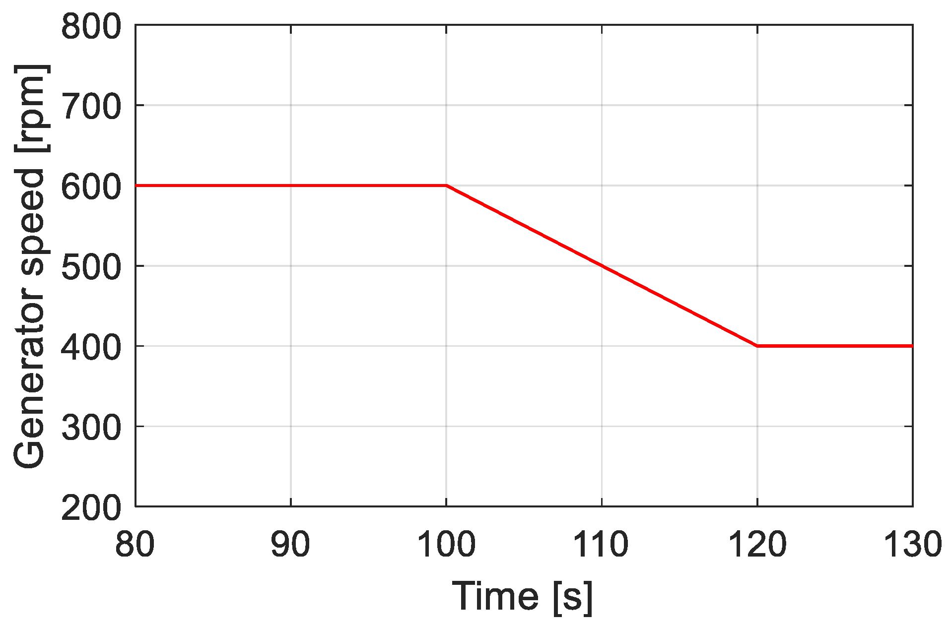
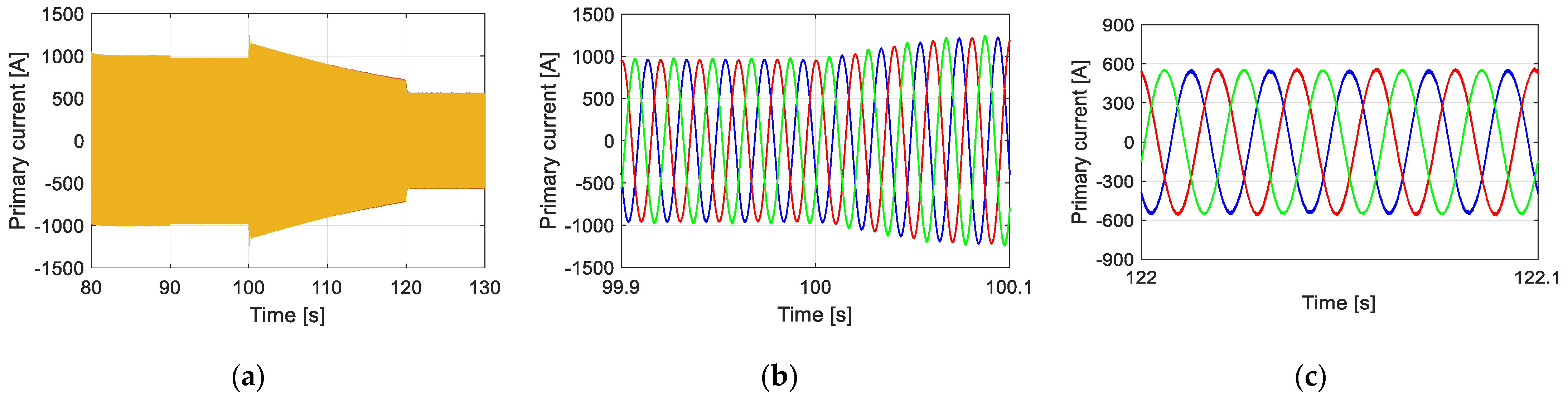
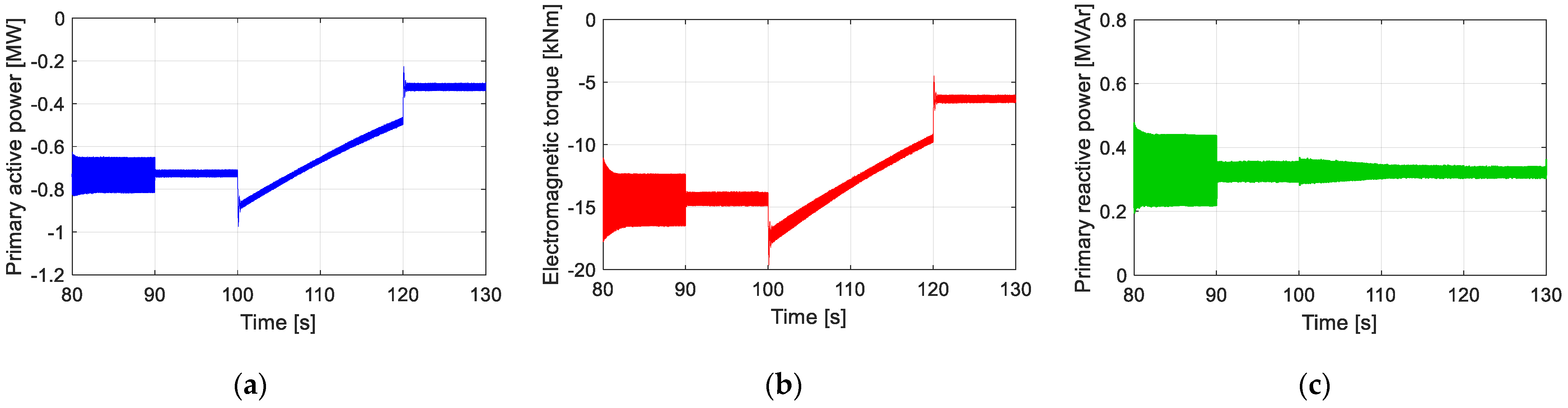
In order to test the performance of the proposed control during operation under variable speed and loading conditions (load change in accordance with (52)), the speed mode change from super to sub-synchronous was analyzed. The test was conducted with the maximum power point tracking (MPPT).
Under the
Target I, the primary current remained balanced during the transient and the new steady state, as clearly seen in
Figure 18. During the speed change, the primary active power was well controlled according to the
Target II requirements as shown in
Figure 19a. Good torque response can be also observed from
Figure 19b during the transient period between super- and sub-synchronous speeds according to the
Target III. On the other hand, the reactive power remained constant as is expected under the MTPIA.
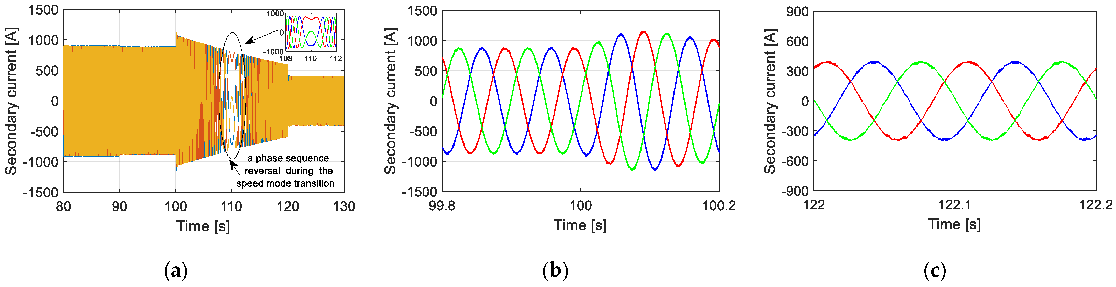
Furthermore,
Figure 20 shows a phase sequence reversal while changing from super- to sub-synchronous speed modes, with a good performance under the
Target IV.


