Comparative Study of Classical and MPC Control for Single-Phase MMC Based on V-HIL Simulations

Abstract

The operation of single-phase Modular Multilevel Converter (MMC) is analyzed in the paper. A mathematical model of the converter is developed and described, based on which the structure and selection of parameters for Classical Control and Optimal Switching State Model Predictive Control (OSS-MPC) are defined. Additionally, the procedure for the determination of circuit parameters, such as submodule capacitance and arm inductance, is described and carried out. The listed control methods are designed and evaluated in Virtual Hardware-in-the-Loop together with single-phase MMC power circuit, regarding three control objectives: AC current control, voltage balancing control and circulating current control. Control methods are evaluated for both steady-state and transient performance and compared based on nine criteria: AC current reference tracking, THD of AC current and voltage, submodule capacitor voltage balancing, total submodule voltage control, circulating current magnitude and THD, number of control parameters and computational complexity. This is the first time that a fair comparison between Classical Control and MPC is considered in literature, resulting in superior performance of both control methods regarding four different criteria and the same performance regarding AC current reference tracking.

1. Introduction

In accordance with the ever growing energy demands, together with the depletion and combustion problems of fossil fuels, renewable energy sources, especially large offshore wind farms have gained maybe the most significant place in future energy systems. Since 2002, when the modular multilevel converter (MMC) was proposed [1], it is recognized as the most attractive solution for HVDC transmission systems of offshore wind farms but also in other HVDC applications, as well as in industry. In the last two decades, intense research work was invested in MMCs and systematized in several recently published review papers, such as [2,3,4,5]. The authors of [3] have presented the state of the art of MMCs regarding topologies, modeling and control methods, modulation techniques and applications. The authors of [2] have additionally discussed power losses considering the wide-bandgap (WBG) technology application. A review of operation and control methods for MMCs in unbalanced AC grids is provided in [4], while [5] presents the state of the art in model predictive control of high power MMCs. Considering AC-to-AC applications, the state of the art in relatively new power converter topology—modular multilevel matrix converters has been discussed regarding implementation issues and applications [6]. As stated in listed literature, the MMC is the preferable topology for high power and medium/high voltage energy conversion systems, because it offers modularity, voltage and current scalability, high efficiency with transformer—less operation, redundancy at low expenses and reduced output current ripple. Consequently, the filter size is reduced, but because of their complexity, MMCs are challenging from the control standpoint.

There are many control objectives that need to be met for the converter to operate properly, including AC current, circulating current and energy balancing between the submodules [7,8]. In addition, circuit parameters need to be defined and optimally chosen [9,10,11]. Throughout the years, various approaches for MMC control have been reported and can be mainly classified as classical methods and model predictive control (MPC) methods according to [3]. While the operation and performance of a MMC with applied Classical Control depends on the modulation method, switching frequency and proportional-integral (PI) control design and tuning, the application of MPC methods offers to overcome the limitations of Classical Control by attaining numerous control objectives with a single cost function [3]. Likewise, the MMC as a switching converter represents a nonlinear system possessing multiple coupled variables [2]. Therefore, the implementation of conventional (classical) methods has limitations regarding the dynamic response that can be overcome by applying nonlinear and predictive control strategies such as MPC. MPC can handle multiple constrains in a single cost function, providing fast dynamic response and high robustness regarding parameter variations and external disturbances [2]. Besides that, there are numerous other inventions introduced in literature to overcome limitations of classical control methods among which is the application of fractional-order PID (FOPID) controllers with non-integer derivation and integration [12,13]. FOPID controllers provide reduced THD of the output current, reduced amplitude and phase errors by controlling the switching frequency of the output voltage, good dynamic response and excellent start-up response, but their main disadvantage is complex design and tuning compared to traditional PID controllers [12].

For the single-phase MMC considered in the papers, there are two methods that can be applied: Optimal Voltage Level Model Predictive Control (OVL-MPC) and Optimal Switching State Model Predictive Control (OSS-MPC) [12]. The OVL-MPC has a single cost function that regulates AC current and circulating current. It generates an optimal number of submodules in the arm that need to be “inserted”, and based on that information voltage (energy) balancing block determines exactly which submodules are going to be “inserted” [12,14]. OSS-MPC also uses a single cost function, but voltage balancing is integrated into the function. Therefore, OSS-MPC is a more precise method compared to OVL-MPC, but also more computationally complex.

In order to maintain the good characteristics of MPC methods while reducing computational complexity, there are several methods which combine MPC with Classical Control and other control mechanisms. Implementation of Neural Network based MPC is presented in [15]. Combination of Nearest Level Control (NLC) and MPC is described in [16], while the impact of submodules grouping on MMC performance is analyzed in [17]. Merging of Classical Control and MPC into deadbeat control is presented in [18]. The MPC method that has the ability to determine online optimal trajectory for the single-phase MMC is presented in [19].

There is a notable lack of literature regarding the fair quantitative comparison between MPC and classical MMC control, in addition to listed qualitative differences, which this paper aims to fill. It is necessary to define adequate criteria for determining the improvement in MMC performance obtained by introducing MPC-based control algorithms compared to Classical Control. This paper is focused on conducting this comparison, thereby facilitating the choice of a control methods combination which results in the best performance of single-phase MMCs.

In this paper, Classical Control and OSS-MPC are designed and evaluated. Based on evaluation results, these methods are compared. For the purposes of analysis conducted in the paper, implementations of Classical Control and OSS-MPC methods for a single-phase MMC are evaluated using Typhoon’s Virtual Hardware-in-the-Loop (V-HIL). In both cases controllers and single-phase MMC are modeled in V-HIL that represents a useful tool to evaluate converter operation and to test control performance prior to converter design and assembly. Owing to the working principle of V-HIL, each model can contain a certain number of switches. V-HIL 402, supporting up to 12 switching modules, is used in the research presented in the paper. In the case of a greater number of submodules per arm, would need to be arms are modeled by an equivalent circuit. The disadvantage of such a modeling approach is that it is impossible to access and control individual submodules. Therefore, a single-phase MMC with six submodules per arm is analyzed and evaluated in the paper. Both control methods are based on precisely defined mathematical models, which helps determine the optimal number and values of control parameters [7,8].

An overview of single-phase MMCs with mathematical model description and circuit parameter setting is given in Section 2. Section 3 is dedicated to Classical Control analysis. Control mechanisms of OSS-MPC are analyzed in Section 4. Evaluation and comparison of these methods are located in Section 5. Finally, the conclusions are derived in Section 6.

2. MMC Overview

Mathematical model of the selected single-phase MMC topology is derived in this section, based on which control objectives are defined. In addition, the procedure for submodule capacitance and arm inductance selection is described and performed, in order to ensure appropriate operation of MMC.

2.1. Topology

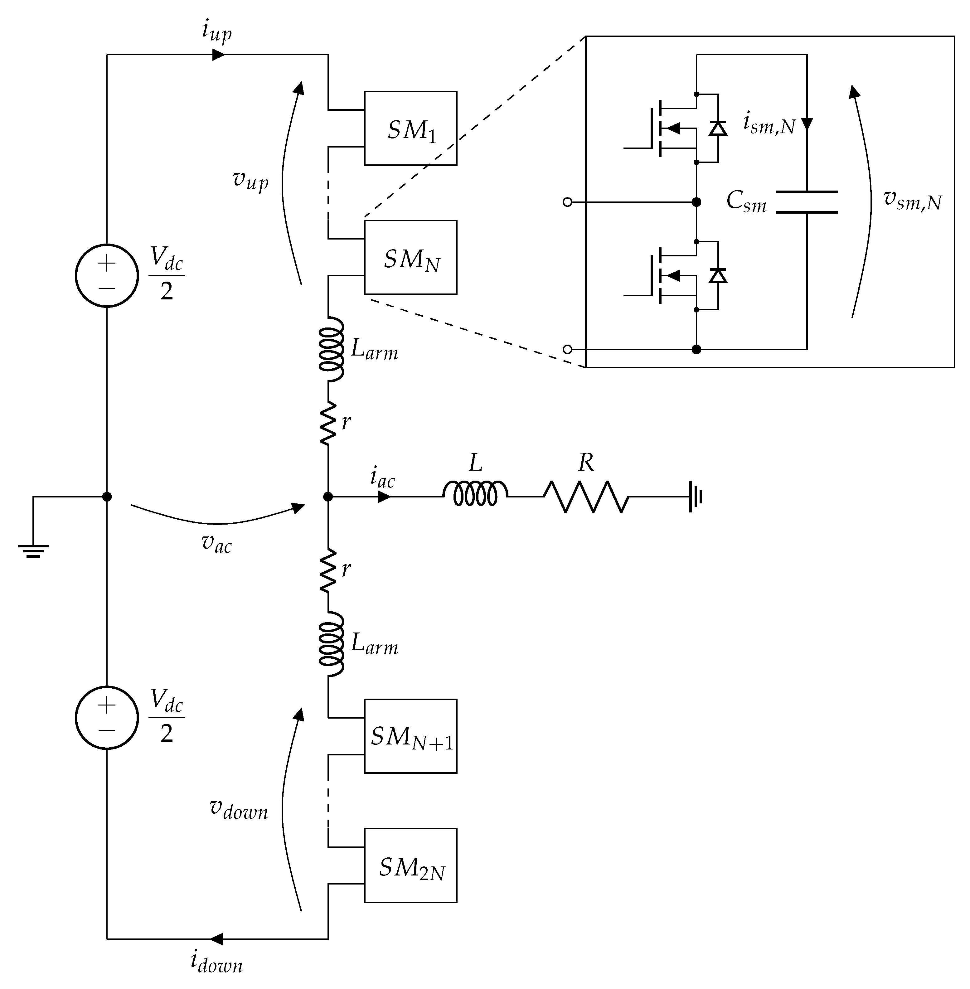
Single-phase MMC topology is presented in Figure 1. This converter consists of one leg and the leg is composed of two arms. In the middle of the arm is the AC terminal, connected to $R-L$ load. Each arm consists of N submodules. There are different variants for submodule topology, such as Half-Bridge, Full-Bridge, etc. [7]. Due to the limited model complexity allowed by the applied HIL device, i.e., the maximum number of switches per circuit, the Half-Bridge topology is chosen for the submodules, as shown in Figure 1.

The Half-Bridge submodule consists of a single capacitor in parallel with two switches. These switches have complementary control logic; when the upper switch is on, the lower switch is turned off, and vice versa. When the upper switch is on, the voltage between terminals of the submodule is equal to the capacitor voltage, and the capacitor is exposed to the arm current. When the lower switch is on, the submodule terminals are shorted and there is no current flowing through the capacitor. Therefore, it can be concluded that the capacitor voltage will increase if the arm current is positive and decrease if the arm current is negative when the upper submodule switch is turned on. When the lower submodule switch is turned on, the capacitor voltage does not change.

The number of “inserted” submodules (submodules with upper switch turned on) determines the arm voltage. The sum of arm voltages determines DC voltage of the leg, whereas their difference “generates” the voltage at the AC terminal.

2.2. Mathematical Model

According to single-phase MMC topology presented in Figure 1, it can be concluded that voltages $v_{up}$ and $v_{down}$ are equal to:

$$v_{up}=\frac{V_{dc}}{2}-L_{arm}\frac{\mathrm{d}{i}_{up}}{\mathrm{d}t}-r{i}_{up}-v_{ac},$$

(1)

$$v_{down}=\frac{V_{dc}}{2}-L_{arm}\frac{\mathrm{d}{i}_{down}}{\mathrm{d}t}-r{i}_{down}+v_{ac}.$$

(2)

The half-sum of arm currents determines the circulating current $i_z$:

$$i_z=\frac{i_{up}+i_{down}}{2},$$

(3)

whereas the difference between these two currents is equal to the AC current $i_{ac}$:

$$i_{ac}=i_{up}-i_{down}.$$

(4)

From (3) and (4), upper and lower arm currents $i_{up}$ and $i_{down}$ can be expressed as:

$$i_{up}=i_z+\frac{i_{ac}}{2},$$

(5)

$$i_{down}=i_z-\frac{i_{ac}}{2}.$$

(6)

By combining (5) and (6) with (1) and (2), (7) and (8) can be obtained:

$$v_{up}=\frac{V_{dc}}{2}-L_{arm}\frac{\mathrm{d}{i}_z}{\mathrm{d}t}-\frac{L_{arm}}{2}\frac{\mathrm{d}{i}_{ac}}{\mathrm{d}t}-r{i}_z-\frac{r}{2}{i}_{ac}-v_{ac},$$

(7)

$$v_{down}=\frac{V_{dc}}{2}-L_{arm}\frac{\mathrm{d}{i}_z}{\mathrm{d}t}+\frac{L_{arm}}{2}\frac{\mathrm{d}{i}_{ac}}{\mathrm{d}t}-r{i}_z+\frac{r}{2}{i}_{ac}+v_{ac}.$$

(8)

The half-difference of $v_{down}$ and $v_{up}$, which is basically the arm voltage component that generates voltage at the AC terminal, can be obtained by subtracting (7) from (8):

$$v_{\delta }=\frac{v_{down}-v_{up}}{2}=v_{ac}+\frac{L_{arm}}{2}\frac{\mathrm{d}{i}_{ac}}{\mathrm{d}t}+\frac{r}{2}{i}_{ac}.$$

(9)

AC load voltage $v_{ac}$ is also equal to:

$$v_{ac}=L\frac{\mathrm{d}{i}_{ac}}{\mathrm{d}t}+R{i}_{ac}.$$

(10)

By combining the previous two equations, the following expression for arm voltages half-difference $v_{\delta }$ is derived:

$$v_{\delta }=(L+\frac{L_{arm}}{2})\frac{\mathrm{d}{i}_{ac}}{\mathrm{d}t}+(R+\frac{r}{2})i_{ac}.$$

(11)

AC voltage references for upper and lower arm voltages $v_{\delta ,up}^{*}$ and $v_{\delta ,down}^{*}$ have the same values, but are of opposite sign:

$$v_{\delta ,down}^{*}=-v_{\delta ,up}^{*}=v_{\delta }^{*}=(L+\frac{L_{arm}}{2})\frac{\mathrm{d}{i}_{ac}^{*}}{\mathrm{d}t}+(R+\frac{r}{2})i_{ac}^{*},$$

(12)

where $i_{ac}^{*}$ is AC current reference. On the other hand, leg voltage $v_{\mathsf{\Sigma }}$ is obtained by adding (8) to (7):

$$v_{\mathsf{\Sigma }}=v_{up}+v_{down}=V_{dc}-2L_{arm}\frac{\mathrm{d}{i}_z}{\mathrm{d}t}-2r{i}_z.$$

(13)

Arm voltages can be decoupled in the same way as arm currents:

$$v_{up}=\frac{v_{\mathsf{\Sigma }}}{2}-v_{\delta },$$

(14)

$$v_{down}=\frac{v_{\mathsf{\Sigma }}}{2}+v_{\delta }.$$

(15)

The DC arm voltage reference $v_{\mathsf{\Sigma }}^{*}$ consists of half the value of DC-link voltage $V_{dc}/2$ and compensating voltage $v_z^{*}$:

$$\frac{v_{\mathsf{\Sigma }}^{*}}{2}=\frac{V_{dc}}{2}-v_z^{*}.$$

(16)

Compensating voltage $v_z^{*}$ controls the circulating current $i_z^{*}$:

$$v_z^{*}=L_{arm}\frac{\mathrm{d}{i}_z^{*}}{\mathrm{d}t}+r{i}_z^{*}.$$

(17)

Finally, reference voltages for upper and lower arm are given by the following two equations:

$$v_{up}^{*}=\frac{V_{dc}}{2}-v_{\delta }^{*}-v_z^{*},$$

(18)

$$v_{down}^{*}=\frac{V_{dc}}{2}+v_{\delta }^{*}-v_z^{*}.$$

(19)

When (12) and (17) are combined with (18)–(21) are obtained:

$$v_{up}^{*}=\frac{V_{dc}}{2}-(L+\frac{L_{arm}}{2})\frac{\mathrm{d}{i}_{ac}^{*}}{\mathrm{d}t}-(R+\frac{r}{2})i_{ac}^{*}-L_{arm}\frac{\mathrm{d}{i}_z^{*}}{\mathrm{d}t}+r{i}_z^{*},$$

(20)

$$v_{down}^{*}=\frac{V_{dc}}{2}+(L+\frac{L_{arm}}{2})\frac{\mathrm{d}{i}_{ac}^{*}}{\mathrm{d}t}+(R+\frac{r}{2})i_{ac}^{*}-L_{arm}\frac{\mathrm{d}{i}_z^{*}}{\mathrm{d}t}-r{i}_z^{*}.$$

(21)

If AC current is required to be a sine function:

$$i_{ac}^{*}=I_{ac}^{*}sin(\omega t),$$

(22)

then (20) and (21) can be modified to obtain (23) and (24):

$$v_{up}^{*}=\frac{V_{dc}}{2}-Z{I}_{ac}^{*}sin(\omega t+\phi )-L_{arm}\frac{\mathrm{d}{i}_z^{*}}{\mathrm{d}t}+r{i}_z^{*},$$

(23)

$$v_{down}^{*}=\frac{V_{dc}}{2}+Z{I}_{ac}^{*}sin(\omega t+\phi )-L_{arm}\frac{\mathrm{d}{i}_z^{*}}{\mathrm{d}t}-r{i}_z^{*},$$

(24)

where Z is equal to:

$$Z=\sqrt{{\omega }^2{(L+\frac{L_{arm}}{2})}^2+{(R+\frac{r}{2})}^2},$$

(25)

while $\phi$ is equal to:

$$\phi =arctan{\displaystyle \frac{\omega (L+{\displaystyle \frac{L_{arm}}{2}})}{R+{\displaystyle \frac{r}{2}}}}.$$

(26)

It should be noted that the product $Z{I}_{ac}^{*}$ must be smaller then the half of the DC link voltage. If it is assumed that circulating current has no AC component and that the number of submodules and switching frequency have no effect on upper and lower arm voltages, then upper and lower arm voltage equations can be written as:

$$v_{up}=\frac{V_{dc}}{2}-Z{I}_{ac}sin(\omega t+\phi )-r{I}_z,$$

(27)

$$v_{down}=\frac{V_{dc}}{2}+Z{I}_{ac}sin(\omega t+\phi )-r{I}_z,$$

(28)

where $I_z$ is DC value of circulating current $i_z$. Arm currents can be expressed as:

$$i_{up}=I_z+\frac{I_{ac}}{2}sin\left(\omega t\right),$$

(29)

$$i_{down}=I_z-\frac{I_{ac}}{2}sin\left(\omega t\right).$$

(30)

Consequently, instantaneous upper arm power is defined as:

$$p_{up}\left(t\right)=v_{up}\left(t\right)i_{up}\left(t\right)=(\frac{V_{dc}}{2}-Z{I}_{ac}sin(\omega t+\phi )-r{I}_z)(I_z+\frac{I_{ac}}{2}).$$

(31)

The average value of $p_{up}$ corresponds to active power in upper submodules:

$$P_{up}=\frac{V_{dc}{I}_z}{2}-\frac{Z{I}_{ac}^2}{4}cos\left(\phi \right)-r{I}_z^2.$$

(32)

Knowing that $P_{up}$ is equal to zero in steady-state, one can calculate the circulating current reference as in (33):

$$I_z^{*}={\displaystyle \frac{{\displaystyle \frac{V_{dc}}{2}}-\sqrt{{\displaystyle \frac{V_{dc}^2}{4}}-rZ{I}_{ac}^{*2}cos\left(\phi \right)}}{2r}}.$$

(33)

2.3. Control Objectives

There are three control objectives that are considered in this paper: AC current control, voltage balancing control and circulating current control. In order to tune the controller properly, appropriate MMC state-space models will be defined. It is also necessary to define the discrete form of state-space model equations to allow MPC implementation. Forward Euler approximation is used for converting continuous-time model to discrete-time model.

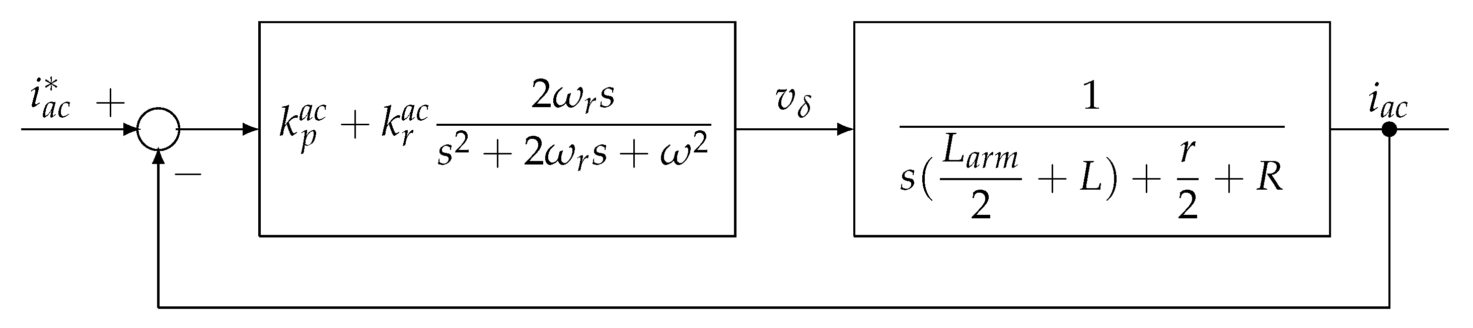
2.3.1. AC Current Control

The differential equation that describes AC current behavior is given as:

$$\frac{v_{down}-v_{up}}{2}=({\displaystyle \frac{L_{arm}}{2}}+L){\displaystyle \frac{\mathrm{d}{i}_{ac}}{\mathrm{d}t}}+({\displaystyle \frac{r}{2}}+R)i_{ac}.$$

(34)

The discrete form of the previous equation is given as:

$$i_{ac}(k+1)={\mathsf{\Phi }}_{ac}{i}_{ac}\left(k\right)+{\mathsf{\Gamma }}_{ac}\frac{v_{down}\left(k\right)-v_{up}\left(k\right)}{2},$$

(35)

where parameters ${\mathsf{\Phi }}_{ac}$ and ${\mathsf{\Gamma }}_{ac}$ are equal to:

$${\mathsf{\Phi }}_{ac}=\left(1-{\displaystyle \frac{{\displaystyle \frac{r}{2}}+R}{{\displaystyle \frac{L_{arm}}{2}}+L}}\right)T_s,$$

(36)

$${\mathsf{\Gamma }}_{ac}={\displaystyle \frac{T_s}{{\displaystyle \frac{L_{arm}}{2}}+L}},$$

(37)

and $T_s$ is the sampling period.

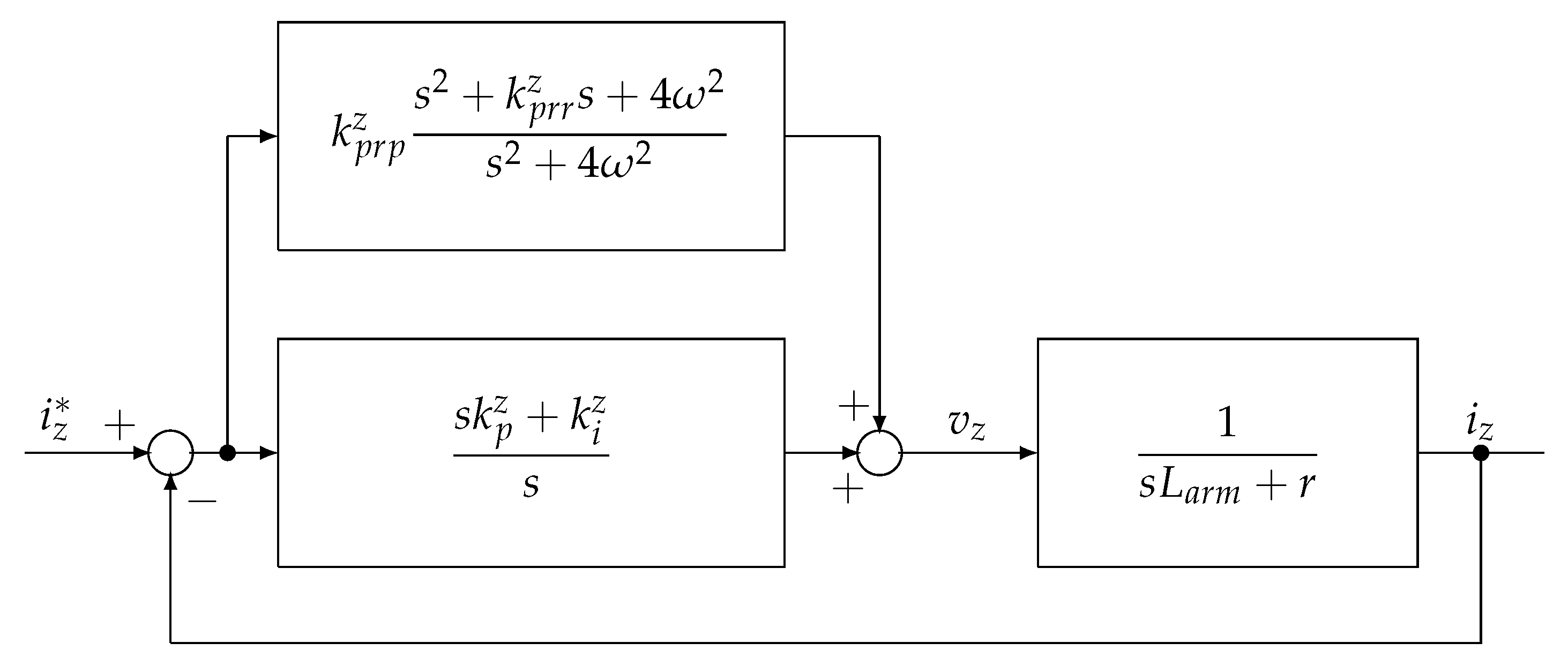
2.3.2. Circulating Current Control

The circulating current differential equation in continuous form is given as:

$$V_{dc}-v_{up}-v_{down}=2L_{arm}\frac{\mathrm{d}{i}_z}{\mathrm{d}t}+2r{i}_z.$$

(38)

The discrete form of the previous equation is given as:

$$i_z(k+1)={\mathsf{\Phi }}_z{i}_z\left(k\right)+{\mathsf{\Gamma }}_z\left[V_{dc}-v_{down}\left(k\right)-v_{up}\left(k\right)\right],$$

(39)

where parameters ${\mathsf{\Phi }}_z$ and ${\mathsf{\Gamma }}_z$ are equal to:

$${\mathsf{\Phi }}_z=\left(1-{\displaystyle \frac{r}{L_{arm}}}\right)T_s,$$

(40)

$${\mathsf{\Gamma }}_z={\displaystyle \frac{T_s}{2L_{arm}}}.$$

(41)

2.3.3. Submodule Capacitor Voltage Control

The differential equation that describes the submodule capacitor voltages is given by (42):

$$C_{sm}\frac{\mathrm{d}{v}_{sm,j}}{\mathrm{d}t}=\left\{\begin{array}{cc}{i}_{up},\hfill & 1\le j\le N,\hfill \\ i_{down},\hfill & N+1\le j\le 2N,\hfill \end{array}\right.$$

(42)

where N is the number of submodules per arm, $C_{sm}$ is the submodule capacitance and $v_{sm,j}$ is the capacitor voltage corresponding to the j-th submodule. The discrete form of the previous equation is given as:

$$v_{sm,j}(k+1)=\left\{\begin{array}{cc}{v}_{sm,j}\left(k\right)+{\displaystyle \frac{i_{up}{T}_s}{C}},\hfill & 1\le j\le N,\hfill \\ v_{sm,j}\left(k\right)+{\displaystyle \frac{i_{down}{T}_s}{C}},\hfill & N+1\le j\le 2N.\hfill \end{array}\right.$$

(43)

2.4. Parameter Settings

Initial parameters of single-phase MMC are presented in

Table 1. Initial single-phase MMC parameters.

Parameter Name	Designation	Value
DC bus voltage	$V_{dc}$	3 kV
Number of submodules per arm	N	6
Load resistance	R	80 Ω
Load inductance	L	0.19 H
Switching frequency	$f_{pwm}$	6 kHz
Fundamental AC frequency	f	50 Hz

. Based on these parameters, the submodule capacitance, arm inductance and arm resistance can be selected.

2.5. Submodule Capacitance Selection

Submodule capacitors store the energy within the arm. Equivalent capacitance of one arm is $C_{eq}=C_{sm}/N$, whereas the sum of capacitor voltages within the arm is equal to the DC link voltage. If capacitor voltage ripple is neglected, energy stored within the submodules of the observed arm can be calculated as:

$$E={\displaystyle \frac{C_{eq}{V}_{dc}^2}{2}}={\displaystyle \frac{C_{sm}{V}_{dc}^2}{2N}}.$$

(44)

However, energy fluctuation must be taken into consideration. In fact, the ripple of the voltage across capacitor $C_{eq}$ is proportional to the square root of energy fluctuation and reversely proportional to capacitance $C_{eq}$. Submodule capacitance is chosen according to the voltage ripple requirement [9,20]. Energy fluctuation of the upper arm is obtained by integrating the AC component of instantaneous power given by (31) and adding it to (44), leading to (45):

$$e_{up}\left(t\right)=\frac{C_{sm}{V}_{dc}^2}{2N}+\frac{I_{ac}}{8\omega }F\left(t\right),$$

(45)

where $F\left(t\right)$ is given by:

$$F\left(t\right)=8Z{I}_{z}cos(\omega t+\phi )-2V_{dc}cos\left(\omega t\right)-Z{I}_{ac}sin(2\omega t+\phi )+4r{I}_{z}cos\left(\omega t\right),$$

(46)

and $I_z$ is calculated as:

$$\begin{array}{c}\hfill I_z={\displaystyle \frac{{\displaystyle \frac{V_{dc}}{2}}-\sqrt{{\displaystyle \frac{V_{dc}^2}{4}}-rZ{I}_{ac}^{2}cos\left(\phi \right)}}{2r}}.\end{array}$$

(47)

Assuming an even distribution of energy across the arm, the following holds:

$$\begin{array}{c}\hfill e_{up}\left(t\right)=\frac{N{C}_{sm}{v}_{sm}^2\left(t\right)}{2},\end{array}$$

(48)

where $v_{sm}$ is the voltage of a single submodule. By equalizing (45) and (48), submodule capacitor voltage $v_{sm}\left(t\right)$ is obtained:

$$\begin{array}{c}\hfill v_{sm}\left(t\right)=\sqrt{\frac{V_{dc}^2}{N^2}+\frac{I_{ac}}{4N\omega C_{sm}}F\left(t\right)}.\end{array}$$

(49)

Minimal submodule voltage is equal to:

$$\begin{array}{c}\hfill V_{sm,min}=\sqrt{\frac{V_{dc}^2}{N^2}+\frac{I_{ac}}{4N\omega C_{sm}}{F}_{min}},\end{array}$$

(50)

while maximal submodule voltage is equal to:

$$\begin{array}{c}\hfill V_{sm,max}=\sqrt{\frac{V_{dc}^2}{N^2}+\frac{I_{ac}}{4N\omega C_{sm}}{F}_{max}},\end{array}$$

(51)

where $F_{min}$ and $F_{max}$ are minimum and maximum of $F\left(t\right)$ function. If the submodule voltage variations are limited to $\pm 0.25\%$ of $V_{dc}/N$ reference value, i.e., if the submodule voltage can vary between $0.9975$ $V_{dc}/N$ and $1.0025$ $V_{dc}/N$, submodule capacitance is calculated to be no lower than 9.2 mF. The value of 10 mF is selected for the submodule capacitance $C_{sm}$.

2.6. Arm Inductance Selection

The value of arm inductance influences the harmonic content of circulating current. Namely, by increasing the arm inductance, the circulating current harmonics are decreased. The problem regarding circulating currents in single-phase MMC circuit is that only the DC component has a purpose in active power transfer from DC terminal to AC terminal. Apart from the DC component, second-order harmonic is also present due to imbalance across the leg. This component increases the losses, which is why it should be attenuated.

Arm inductance is selected based on analysis conducted in literature [21]. The choice is guided by two conditions: avoiding resonant frequency and attenuation of circulating current second order harmonic amplitude.

2.6.1. Resonant Frequency

According to [10], the circulating current contains harmonics at frequency $n\omega$, where n is the order of the harmonic, and $\omega$ is the fundamental frequency of the AC circuit. Any higher-order harmonic can cause resonance if $\omega$ is selected so that the following holds [10]:

$$\begin{array}{c}\hfill \omega ={\omega }_{res}=\sqrt{{\displaystyle \frac{N(2n^2-2+m^2{n}^2)}{4L_{arm}{C}_{sm}{n}^2(n^2-1)}}},\end{array}$$

(52)

where $m=2v_{\delta }/V_{dc}$ is modulation index. To avoid resonance for all higher order harmonics, it is desirable to operate the converter at $\omega >{\omega }_{res}$. Maximal resonance frequency occurs when $n=2$ and $m=1$, which imposes the following condition:

$$\begin{array}{c}\hfill L_{arm}{C}_{sm}>\frac{5N}{24{\omega }^2},\end{array}$$

(53)

where $\omega$ is set to 100 $\pi$ rad/s. With $C_{sm}$ already selected, it is concluded that arm inductance has to be $L_{arm}>1.26$ mH.

2.6.2. Circulating Current Second Order Harmonic Amplitude

Based on [10], circulating current second order harmonic amplitude $I_{z2}$ can be estimated as:

$$\begin{array}{c}\hfill I_{z2}=Re\left\{{\displaystyle \frac{-j\left({\displaystyle \frac{3m{I}_{ac}}{8\omega }}{e}^{j\phi }-{\displaystyle \frac{m^2{I}_z}{2\omega }}\right)}{{\displaystyle \frac{4C_{sm}}{N}}(j2\omega L_{arm}+r)-j{\displaystyle \frac{6+4m^2}{12\omega }}}}{e}^{j2\omega t}\right\}.\end{array}$$

(54)

If the modulation index m is equal to 1, MMC generates maximal AC power, and in that case circulating current DC component is $I_z\approx 3$ A. If condition $I_{z2}<0.2I_z$ is introduced and the resistance r is neglected in (54), the minimal required value of $L_{arm}$ is determined to be 5 mH. Based on available data for commercial inductors with current rating of 30 A and inductance greater than 5 mH, it was found that parasitic resistance of such inductor ranges from 45 to 130 mΩ. The arm inductance and resistance are therefore set to 5 mH and 100 mΩ, respectively. When these values are included in (54), condition $I_{z2}<0.2I_z$ is still satisfied.

Based on the calculations performed in this section, all MMC parameters have been determined. The complete list of parameters with their values is presented in

Table 2. Single-phase MMC parameters.

Parameter Name	Designation	Value
DC bus voltage	$V_{dc}$	3 kV
Number of submodules per arm	N	6
Load resistance	R	80 Ω
Load inductance	L	0.19 H
Switching frequency	$f_{pwm}$	6 kHz
Fundamental AC frequency	f	50 Hz
Submodule capacitance	$C_{sm}$	10 mF
Arm inductance	$L_{arm}$	5 mH
Arm resistance	r	100 mΩ

.

3. Classical Control

A Classical Control block diagram for the MMC is presented in Figure 2. There are four major control blocks: AC Current Control, Total Leg Voltage Control, Leg Energy Distribution Control and DC Current Control.

3.1. AC Current Control

For classical control of the three-phase MMC (and in general for control of three-phase inverters), abc to dq transformation is usually used, as the currents are obtained by this transformation are DC quantities in steady state and can be easily controlled using PI regulators. For the control of single-phase MMC, a similar type of control is possible but requires to delay of the measured current by $\pi /2$, so that the original and delayed signals are fed to $\alpha \beta$-to-dq transformation block to obtain DC signals. However, Reference [22] suggests that there are methods for AC current control that show better results. One of them is the application of proportional resonant (PR) controller. Parameters tunning procedure for resonant controllers used in this paper is explained in [23].

The AC current control loop block diagram is shown in Figure 3. The AC current error is fed to the resonant controller, where $k_p^{ac}$, $k_r^{ac}$ are proportional and resonant gain, while ${\omega }_r$ determines the bandwidth around resonant frequency, which in this case is set to fundamental AC current frequency $\omega$. The output of the resonant controller is AC voltage reference $v_{\delta }^{*}$. If the modulation block’s transfer function is represented as a unity gain, actual AC voltage $v_{\delta }$ is equal to the AC voltage reference $v_{\delta }^{*}$.

3.2. Total Leg Voltage Control

The sum of submodule capacitor voltages is fed to the block designated Total Leg Voltage Control in Figure 2. This sum is subtracted from the reference ($2V_{dc}$) and the error is fed to the PI controller. The PI controller output, which is also the output of Total Leg Voltage Control block, represents the circulating current reference $i_z$.

3.3. Circulating Current Control

The input of this control block is the circulating current reference $i_z$, obtained from Total Leg Voltage Control block. The difference between reference $i_z^{*}$ and the actual value of circulating current $i_z$ is fed to a PI controller and PR controller (Figure 4). The PI controller tracks and regulates the DC component, whereas the PR controller tracks and regulates the second-order harmonic. For the purpose of the analysis conducted in the paper, both the PI and PR controller are tuned to provide zero steady-state error at 0 Hz and at the second-order harmonic frequency.

Output of circulating current control block is the compensation voltage reference $v_z^{*}$.

3.4. Leg Energy Distribution Control

Total Leg Voltage Control block controls the average value of submodule voltage, but it is also necessary to control distribution of energy between the arms within the leg.

Each capacitor should follow its voltage reference $V_{sm}^{*}=V_{dc}/N$. However, because of alternating direction of arm current, submodule voltage is fluctuating. When an arm current is positive and a submodule from that arm is “inserted”, its capacitor voltage increases. Similarly, when an arm current is negative and a submodule is “inserted”, its capacitor voltage decreases. Leg Energy Distribution Control block introduces a negative feedback loop for these processes. The control law is represented by the following equations:

$$v_{dt,j}^{*}=\left\{\begin{array}{cc}{k}_B(V_{sm}^{*}-v_{sm,j}),\hfill & (i_{up}>0)\hfill \\ k_B(V_{sm}^{*}-v_{sm,j}),\hfill & (i_{up}\le 0)\hfill \end{array}\right.,1\le j\le N$$

(55)

$$v_{dt,j}^{*}=\left\{\begin{array}{cc}{k}_B(V_{sm}^{*}-v_{sm,j}),\hfill & (i_{down}>0)\hfill \\ k_B(V_{sm}^{*}-v_{sm,j}),\hfill & (i_{down}\le 0)\hfill \end{array}\right.,N+1\le j\le 2N$$

(56)

Outputs of this block are fed directly to the Modulation block.

3.5. Modulation

It is worth noting that Phase-Shifted Pulse Width Modulation (PS-PWM) is used for this control. Each submodule has its own carrier, while there are two arm voltage references, one for the upper and one for the lower arm. Carriers for submodules of the same arm are shifted by ${360}^{\circ }/N$, while carriers for submodules from different arms are shifted by ${360}^{\circ }/2N$. Carrier frequency is equal to $f_{pwm}/2N$ for all carriers.

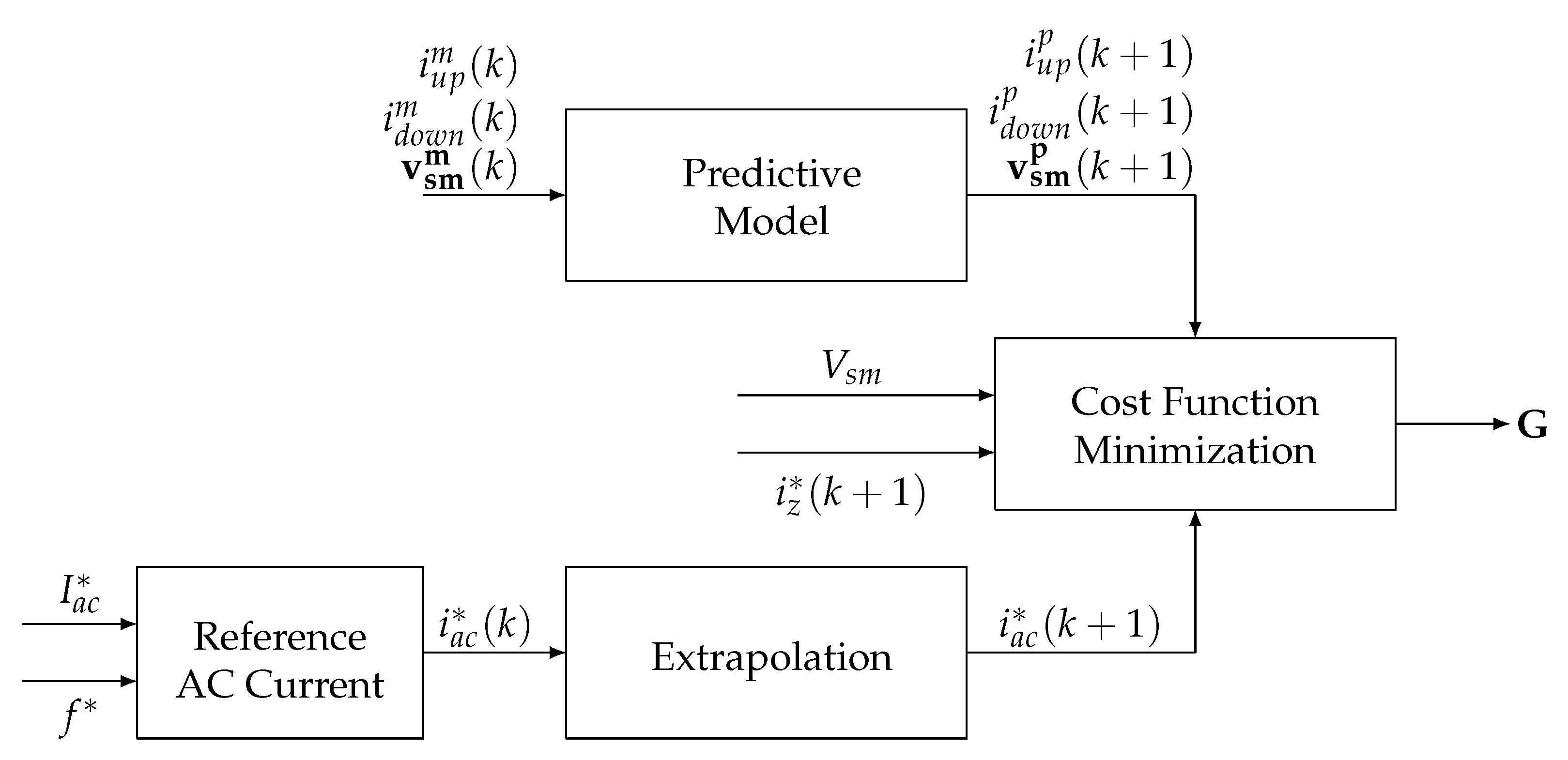
4. OSS-MPC

A block diagram of OSS-MPC method for the MMC is shown in Figure 5. This method is based on a single cost function for two scalars, AC current and circulating current, and one set of variables with $2N$ elements: submodule capacitor voltages. Due to the use of a single cost function, this method is more computationally complex but more precise when compared to the Optimal Voltage Level Model Predictive Method (OVL-MPC), a method also used for control of single-phase MMC [5].

The upper and lower arm currents, $i_{up}\left(k\right)$ and $i_{down}\left(k\right)$, and submodule capacitor voltages $v_{sm,j}$ ($1\le j\le 2N$, array ${\mathbf{v}}_{\mathbf{sm}}$) are measured and fed to Predictive Model block. This block is based on the following expressions:

$$\begin{array}{c}\hfill i_{ac}^p(k+1)={\mathsf{\Phi }}_{ac}{i}_{ac}^m\left(k\right)+{\mathsf{\Gamma }}_{ac}\frac{v_{down}^p\left(k\right)-v_{up}^p\left(k\right)}{2},\end{array}$$

(57)

$$\begin{array}{c}\hfill i_z^p(k+1)={\mathsf{\Phi }}_z{i}_z^m\left(k\right)+{\mathsf{\Gamma }}_z\left[V_{dc}-v_{down}^p\left(k\right)-v_{up}^p\left(k\right)\right],\end{array}$$

(58)

$$v_{sm,j}^p(k+1)=\left\{\begin{array}{cc}{v}_{sm,j}^m\left(k\right)+{\displaystyle \frac{i_{up}^m{T}_s}{C_{sm}}},\hfill & 1\le j\le N,\hfill \\ v_{sm,j}^m\left(k\right)+{\displaystyle \frac{i_{down}^m{T}_s}{C_{sm}}},\hfill & N+1\le j\le 2N.\hfill \end{array}\right.$$

(59)

Equations (57)–(59) are derived from Equations (35), (39) and (43). Voltages $v_{up}^p\left(k\right)$ and $v_{down}^p\left(k\right)$ are input variables, and they depend on the switching state. Designations with m in the exponent represent measured variables. For every switching state there is a single corresponding cost function value. Cost function is calculated as:

$$\begin{array}{c}\hfill f_{crit}={\lambda }_{ac}|i_{ac}^p(k+1)-i_{ac}^{*}(k+1)|+{\lambda }_z|i_z^p(k+1)-i_z^{*}(k+1)|\end{array}{I}_{z,B}+{\lambda }_{sm}\sum _{j=1}^{2N}|v_{sm,j}^p(k+1)-V_{sm}^{*}|,$$

(60)

where ${\lambda }_{ac}$, ${\lambda }_z$ and ${\lambda }_{sm}$ are weighting factors for AC current, circulating current and submodule voltages, respectively. Reference for AC current amplitude $I_{ac}^{*}(k+1)$ determines the circulating current reference $i_z^{*}$ given by Equation (33). In this way, power balance across the MMC is established. Submodule capacitor voltage reference is set to $V_{sm}^{*}=V_{dc}/N$.

Cost function minimization block is used to find a switching state that results in the lowest cost function value. The Switching state with the lowest cost function value is obtained from the cost function minimization block and set as the next switching state $\mathbf{G}$.

5. Results

A single-phase MMC is modeled in Typhoon HIL schematic editor. Along with the power circuit, both Classical Control and OSS-MPC algorithms are designed in separate models. After compiling, each simulation model is loaded into HIL SCADA, in order to extract measurements. Simulation results of steady-state and dynamic performance for each method are presented and discussed in this section.

5.1. Control Parameter Selection

Control parameters for both methods are selected based on the mathematical model of single-phase MMC. For Classical Control, PI controllers are set with damping factor $\zeta =1$ to prevent overshoot. Control parameters used for Classical Control and OSS-MPC are presented in

Table 3. Control parameters for Classical Control.

Parameter Name	Designation	Value
AC current PR controller proportional gain	$k_{prp}^{ac}$	600
AC current PR controller resonant gain	$k_{prr}^{ac}$	20,000
Circulating current PR controller proportional gain	$k_{prp}^z$	753.6
Circulating current PR controller resonant gain	$k_{prr}^z$	2
Circulating current PI controller proportional gain	$k_p^z$	79
Circulating current PI controller integral gain	$k_i^z$	39
Total leg voltage PI controller proportional gain	$k_p^{tlv}$	10
Total leg voltage PI controller integral gain	$k_i^{tlv}$	20
Leg energy distribution control factor	$k_B$	50

and

Table 4. Control parameters for OSS-MPC.

Parameter Name	Designation	Value
AC current weighting factor	${\lambda }_{ac}$	0.95
Circulating current weighting factor	${\lambda }_z$	0.16
Submodule capacitor voltage weighting factor	${\lambda }_{sm}$	1

, respectively.

5.2. Steady-State

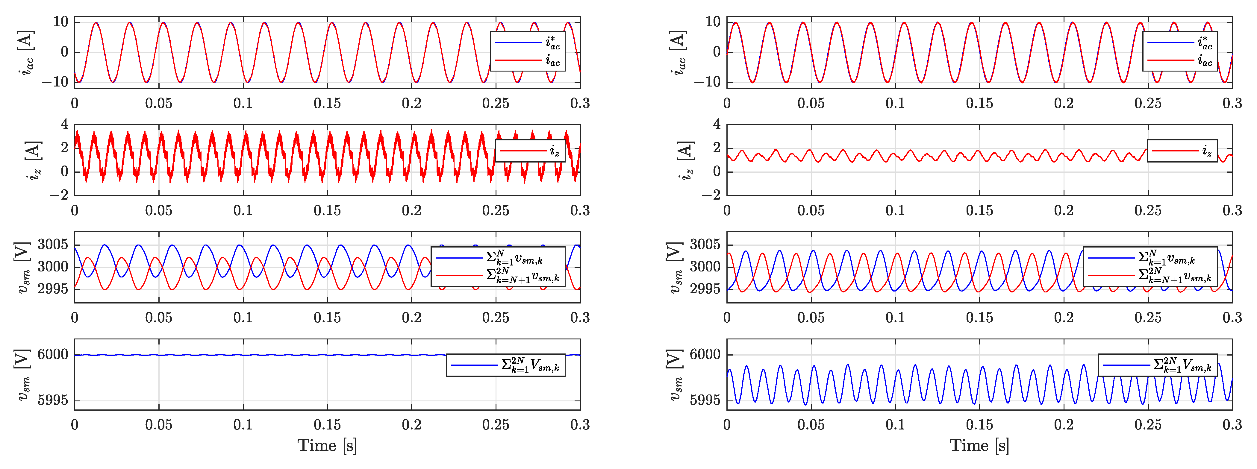
The steady-state results are shown in Figure 6. Each figure contains four time-diagrams: (1) AC current reference and response; (2) circulating current; (3) sums of upper and lower arm submodule voltages; (4) total sum of submodule voltages. Simulation results of Classical Control are presented in four time-diagrams on the left, while OSS-MPC simulation results are presented in four time diagrams on the right.

Regarding the AC current in the steady-state, reference amplitude and frequency are set to 10 A and 50 Hz, respectively. The response tracks the reference precisely in both cases. THD factor of AC voltage $v_{ac}$ for Classical Control and OSS-MPC are equal to 17.74% and 15.93%, respectively. However, THD factors of the AC current for Classical Control is $3.03$%, while for OSS-MPC it equals $1.18$%. These values indicate that in the case of Classical Control, AC voltage contains harmonics of lower order compared to the same voltage obtained when OSS-MPC is used.

OSS-MPC shows superior performance regarding circulating current. Average value of circulating current for both methods is around 1.335 A. However, the presence of second order harmonic is more significant in the case of the Classical Control, yielding a greater peak value of circulating current in the case of Classical Control compared to OSS-MPC.

Regarding submodule capacitor voltages, Classical Control has an advantage over OSS-MPC. In the case of Classical Control, total sum of submodule voltages is tracked almost perfectly, with very little oscillations. The maximal voltage of any of the submodules is 501.01 V, whereas the minimal is 498.95 V. In the case of OSS-MPC, there is a more significant presence of second-order harmonic in total sum of submodules voltage. In addition, the DC component is equal to $2V_{dc}=5996.5$ V rather than the required 6000 V. For OSS-MPC, the maximal voltage of each submodule is 501.17 V, whereas the minimal is 498.46 V.

5.3. Dynamic Performance

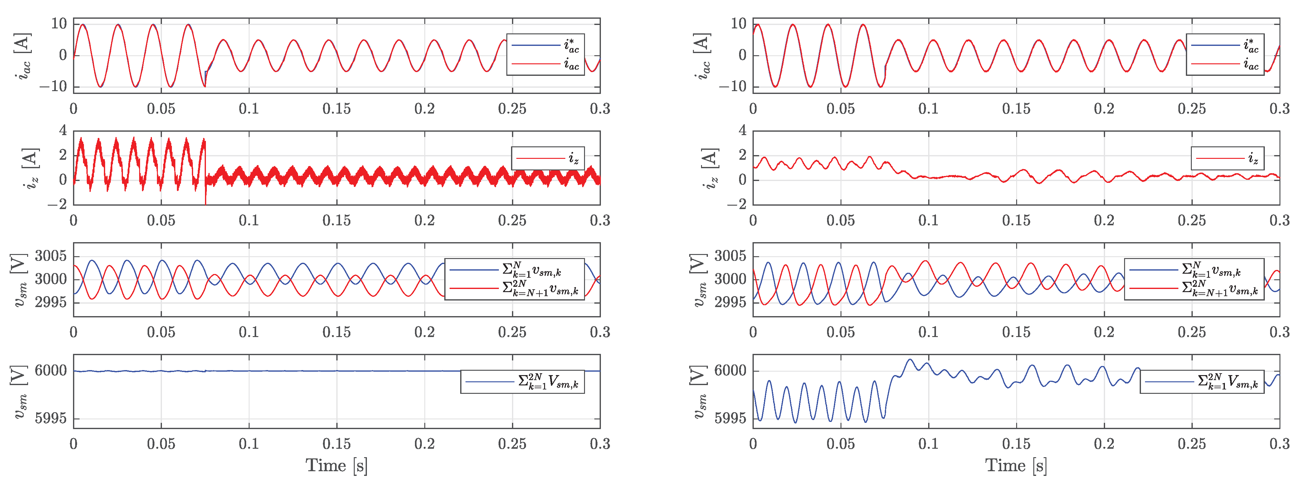
The simulation results of dynamic performance are shown in Figure 7. Similarly to the steady-state results, each figure contains four time-diagrams: (1) AC current reference and response; (2) circulating current; (3) upper and lower arm submodule voltage sums; (4) total sum of submodule voltages. Simulation results of Classical Control are presented in four time-diagrams on the left side, while OSS-MPC simulation results are presented in time-diagrams on the right side.

The following test is performed: amplitude of AC current reference is changed from 10 A to 5 A at $t=0.075$ s. Both control mechanisms responded excellently to the disturbance, as the current continues to track the reference without overshoot or time delay.

Regarding circulating current, similarly to the steady-state operation, a smaller content of second and higher order harmonics is observed in the case of OSS-MPC. As expected, the value of DC component changes for both methods, due to the change in active and reactive power.

Concerning the submodule voltage control, OSS-MPC still has a tracking error after the disturbance, but reduced compared to the previous operating mode. For OSS-MPC, the maximal voltage of each submodule is 502.26 V, whereas the minimal voltage is 498.46 V. In the case of Classical Control, the disturbance causes no significant voltage change. For Classical Control, the maximal voltage of each submodule is 500.94 V, while the minimal voltage is 499.13 V.

Finally, a fair comparison between Classical Control and OSS-MPC Control based on the selected criteria is performed and presented in

Table 5. Classical Control vs. OSS-MPC.

Criteria	Classical Control	OSS-MPC
AC current reference tracking	Excellent	Excellent
AC current THD	3.03%	1.18%
AC voltage THD	15.93%	17.74%
Submodule capacitor voltage balancing	Excellent	Good
Total submodule voltage control	Excellent	Poor
Circulating current tracking	Poor	Good
Circulating current THD	17%	8.8%
Number of control parameters	9	3
Computational complexity	Low	High

.

6. Conclusions

Control strategies for a single-phase MMC are analyzed. Based on this analysis, the submodule capacitance and arm inductance are chosen, as well as the control parameters for two control methods: Classic Control and OSS-MPC. Firstly, an optimal set of parameters is determined for both methods, and the results of simulations performed in Typhoon’s Virtual HIL simulator are compared. This is the first time that a fair comparison is made in the literature, resulting in superior performance of both control methods regarding four different criteria and the same performance regarding AC current reference tracking. Additionally, OSS-MPC is proven to be a better method regarding circulating current which has smaller presence of non-DC components and accordingly reduced value of losses. Concerning voltage control and balancing, Classical Control regulates the sum of submodule voltages almost flawlessly, even when a disturbance is introduced. However, it is worth noting that in the cost function of OSS-MPC, individual submodules’ voltages are regulated rather than their total sum, thus inherently influencing inferior performance of the observed MPC compared to Classical Control.

The authors’ efforts were to fill the void of a fair comparison between Classical Control method and MPC for single-phase MMCs that exists in the literature. The lack of such comparison in the literature may be a consequence of three-phase MMCs being analyzed more extensively due to their preferences in applications. It is required to choose adequate criteria for comparison of Classical Control with other types of control which should introduce improvement in performance of MMC. Therefore, the analysis conducted in the paper emphasizes the significance of this comparison and contributes in indicating the best choice of control methods combination, which should result in the best performance of single-phase MMCs. The authors are planning to extend the research presented in the paper to more robust control analysis and to application of improved control algorithms on FPGA/DSP, which will initially be connected to a HIL emulating power circuit and afterwards to a single-phase MMC experimental setup.