Article

Bayesian Optimized Echo State Network Applied to Short-Term Load Forecasting

by
Gabriel Trierweiler Ribeiro
1,
João Guilherme Sauer
1,
Naylene Fraccanabbia
2,
Viviana Cocco Mariani
1,2 and
Leandro dos Santos Coelho
1,3,*
1
Department of Electrical Engineering, Federal University of Parana (UFPR), Av. Coronal Francisco Heráclito dos Santos, 100, Curitiba (PR) 80060-000, Brazil
2
Department of Mechanical Engineering, Pontifical Catholic University of Parana (PUCPR), Rua Imaculada Conceição, 1155, Curitiba (PR) 80215-901, Brazil
3
Industrial and Systems Engineering Graduate Program (PPGEPS), Pontifical Catholic University of Parana (PUCPR), Rua Imaculada Conceição, 1155, Curitiba (PR) 80215-901, Brazil
*
Author to whom correspondence should be addressed.
Energies 2020, 13(9), 2390; https://doi.org/10.3390/en13092390
Submission received: 29 March 2020 / Revised: 28 April 2020 / Accepted: 30 April 2020 / Published: 11 May 2020
(This article belongs to the Section F: Electrical Engineering)

Abstract

:
Load forecasting impacts directly financial returns and information in electrical systems planning. A promising approach to load forecasting is the Echo State Network (ESN), a recurrent neural network for the processing of temporal dependencies. The low computational cost and powerful performance of ESN make it widely used in a range of applications including forecasting tasks and nonlinear modeling. This paper presents a Bayesian optimization algorithm (BOA) of ESN hyperparameters in load forecasting with its main contributions including helping the selection of optimization algorithms for tuning ESN to solve real-world forecasting problems, as well as the evaluation of the performance of Bayesian optimization with different acquisition function settings. For this purpose, the ESN hyperparameters were set as variables to be optimized. Then, the adopted BOA employs a probabilist model using Gaussian process to find the best set of ESN hyperparameters using three different options of acquisition function and a surrogate utility function. Finally, the optimized hyperparameters are used by the ESN for predictions. Two datasets have been used to test the effectiveness of the proposed forecasting ESN model using BOA approaches, one from Poland and another from Brazil. The results of optimization statistics, convergence curves, execution time profile, and the hyperparameters’ best solution frequencies indicate that each problem requires a different setting for the BOA. Simulation results are promising in terms of short-term load forecasting quality and low error predictions may be achieved, given the correct options settings are used. Furthermore, since there is not an optimal global optimization solution known for real-world problems, correlations among certain values of hyperparameters are useful to guide the selection of such a solution.

1. Introduction

To supply enough energy, operate, and maintain a power system efficiency as well as to trade energy profitably, it is necessary to know how much power will be demanded—that is, it is important to forecast the power system load, a task that is traditionally trusted to the experience of statisticians, engineers and experts from electricity industries. However, the growing introduction of renewable distributed energy, for both sources and consumers, has significantly changed the load profiles, so that traditional approaches are not effective anymore.
Load forecasting task is essential in recent smart energy management systems and it plays a part in the formulation of economic and reliable strategies for power systems. Besides, accurate load forecasting is critical for power system planning and operational decision making. Nevertheless, recent approaches to load forecasting consume a huge amount of available load time series data to produce machine learning models for load forecasting such as deep learning neural networks [1,2,3,4,5,6], ensemble of artificial neural networks [7,8,9,10,11,12], single artificial neural networks [13,14,15,16], Gaussian process [17], long short-term memory networks (LSTM) [18,19,20,21,22], deep belief networks [23,24], heterogeneous ensemble methods [25,26,27,28], k-nearest neighbor [29], echo state network [30,31], deep echo state network [32,33], ensemble of echo state networks [34], extreme learning machines [35,36], ensemble learning of regression trees [37], support vector machines tuned with particle swarm optimization (PSO) algorithm [38], and optimized artificial neural networks [39,40,41,42,43]. A review may be found in [44,45], several machine learning algorithms were compared in [46] and a meta-learning approach was proposed in [47]. A recent publication [48] presents data science methods for wind energy forecasting that could be extended for load forecasting, including autoregressive moving average models, support vector machines, and Artificial Neural Networks (ANNs).
With the development of artificial neural networks, several forecasting models based on ANNs are proposed to enhance the forecasting accuracy of nonlinear time series—for example, the Echo State Network (ESN), which is a type of reservoir for recurrent neural network trained through the learning approach of reservoir computing. The original ESN concept used randomly fixed created reservoirs, and this concept is considered to be one of the main advantages of this effective dynamic neural network model. One advantage of ESN compared to other feed-forward and recurrent ANNs are that only the connections between the reservoir and the output layer need to be trained, thereby reducing the computational complexity for the training phase and making it less likely to get trapped in local optima. Also, ESNs are one of the most well-known types of recurrent neural networks because of their excellent performance when nonlinear dynamic system modeling. It is capable to learn the complex nonlinear behaviors of dynamical systems and these have been successfully applied to a wide range of engineering problems, including time series forecasting [49,50,51] and load forecasting [30,52,53,54,55,56] problems.
ESN uses an interconnected recurrent grid of processing neurons called a dynamical reservoir to replace the hidden layer of classical recurrent neural networks. The basic idea of the ESN is a supervised learning scheme to transform the low dimensional temporal input into a higher dimensional echo state, and then train the output connection weights to make the system output the desired information. However, the use of ESN requires initially the definition of a set of parameters, and this may be done through a trial and error approach or optimization of hyperparameters. In the case of hyperparameter optimization, it is carried out chiefly through metaheuristics, including evolutionary computation and swarm intelligence algorithms. In [52], the Bayesian optimization of Gaussian process hyperparameters in reservoir computing is proposed and the results over two benchmarks, the prediction of a chaotic laser system and a Nonlinear Auto Regressive Moving Average (NARMA) model show that the method is robust. The types of the reservoir considered in their experiments were the dynamic nonlinear delay nodes and the ESN. A variation in the Bayesian optimization of ESNs is proposed in [53].
Like most machine learning algorithms, ESNs possess several hyperparameters of the dynamic reservoir that have to be carefully tuned to achieve a better performance. The ESN approach adopted in this paper has seven hyperparameters: spectral radius, internal units, input scaling, input shift, teacher scaling, teacher shift, and feedback scaling.
Bayesian optimization algorithms (BOAs) applied to echo state networks are found in the literature with two different goals: parameter optimization and hyperparameter optimization. The works in [57,58,59,60] employ the BOA for training the ESN parameters (read-out weights), while [61] employs the BOA for tuning ESN hyperparameters. However, in [61], there is no concern for or investigations about the selection of the acquisition function set in the BOA and experiments are based on theoretical benchmarks.
Like [61], the main contribution of this paper is the investigation of BOA based on the Gaussian process to find suitable hyperparameters of ESN, but applied to short-term load forecasting problems and with additional contributions as follows: (a) the validation of the surrogate utility function known as acquisition function using three approaches, which are expected improvement, lower confidence bound and the probability of improvement. The mentioned approaches were validated in BOA design to reduce forecasting errors and improve the generalization of ESN. (b) A comparison of the proposed ESN model based on BOA with three support vector regression approaches; ESN models achieve better forecasting performance in terms of mean square error minimization on two real-world case studies of short-term load forecasting, one from Poland and another from Brazil. Short-term load forecasting, the forecasting of load ranging from one hour to one week ahead, plays an essential role in the safe and stable operation of the electric grid and has always been a vital research issue for energy management. In this perspective, it could be useful to improve management efficiency and reduce the grid operating cost in power systems.
The remaining parts of this study are organized as follows. Section 2 gives a theoretical background for ESN and the BOA. Followed by an explanation of the proposed ESN approach, the findings are presented in Section 3 and discussed in Section 4. Finally, Section 5 presents the paper’s conclusions and future research directions.

2. Background

This section gives an overview of ESNs, including their basic theory and hyperparameters. Moreover, the fundamentals of BOA are presented.

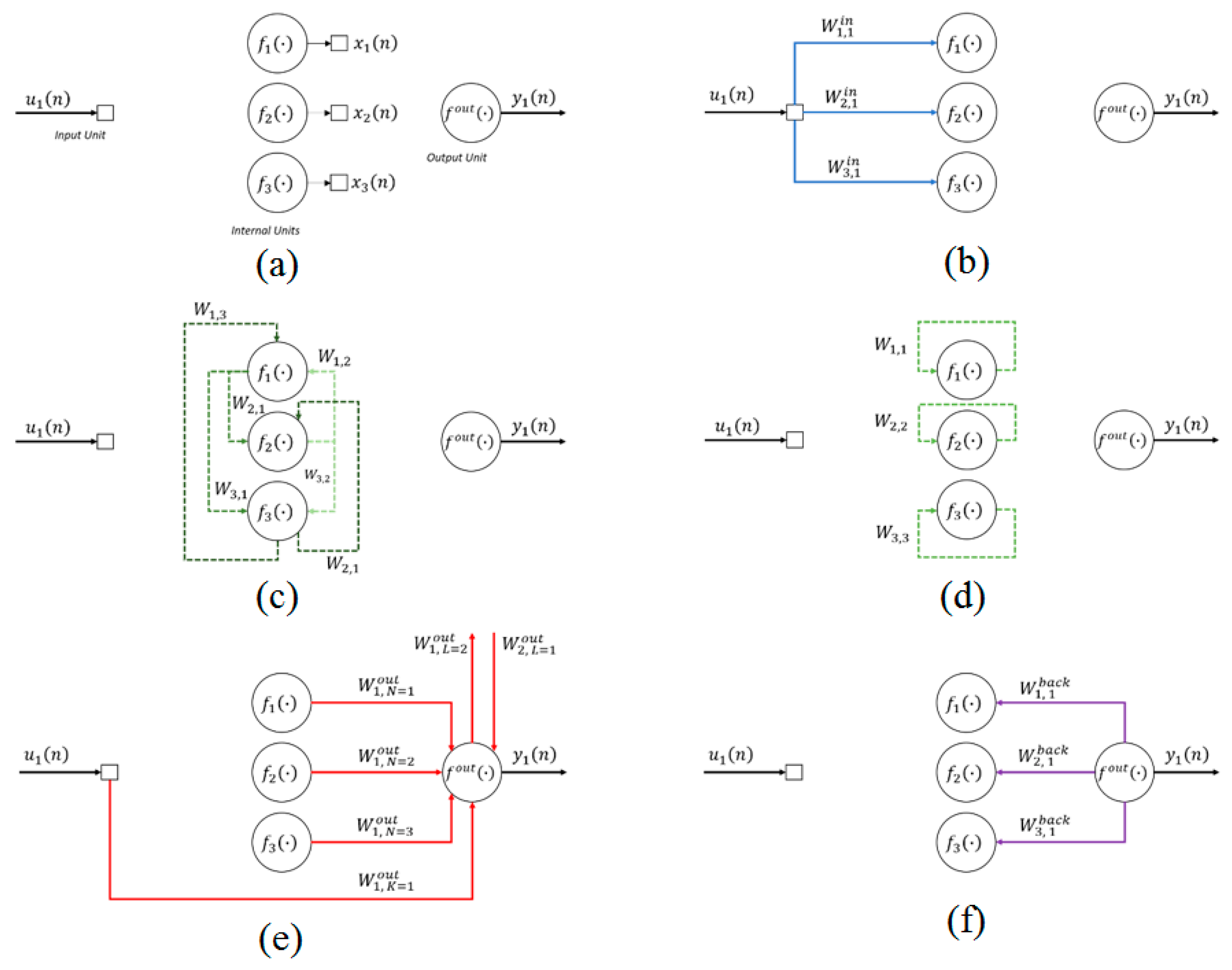
2.1. Echo State Networks

Recurrent Neural Networks (RNNs) are ANNs with recurrent weights—that is, neuron outputs from forward layers may be weighed as inputs to neurons from backward layers, creating a sort of internal memory in the network, making this a non-linear dynamic system (which is an advantage), subject to difficulties in the learning process, likely leading to problems than may be without or slower convergence [54] (which are disadvantages).
Reservoir computing has emerged in recent years as an alternative to gradient descent methods for training RNNs. They have a “reservoir” of dynamics that can be easily tapped to process complex temporal data. ESN is a type of RNN, part of the reservoir computing framework that has a sparse reservoir and a simple linear output.
An ESN, as illustrated in Figure 1, uses a least-squares based learning algorithm in a supervised training form to modify only the output weights based on the inputs and reservoir weights previously randomly assigned, first proposed by Herbert Jaeger in 2001 and later corrected in [62]. The ESN is composed of input units u , internal units f , a recurrent layer called reservoir with fixed sparse hidden-to-hidden connections, and output units f o u t . The output of internal units is called the state x (Figure 1a).
Network weights are divided into four categories, they are input weights W i n (Figure 1b), reservoir weights W (Figure 1c,d), output weights W o u t (Figure 1e), and feedback weights from the output W b a c k (Figure 1f).
The input weights are randomly initialized from a uniform distribution within a specified range between −1 and 1. The reservoir weights are fixed during the training stage, and only the output weights need to be adapted. The hidden layer state vector named “reservoir” is composed of fully connected nonlinear neurons. The reservoir outputs are named echo states when the ESN satisfies the echo state property (ESP).
The states of the reservoir are updated according to
x ( n + 1 ) = f ( W i n · u ( n + 1 ) + W · x ( n ) + W b a c k · y ( n ) )
where n is a time series sample, x , u and y are vectors of reservoir states, inputs and outputs respectively, f are the activation functions of the reservoir neurons.
The output signal y is described by
y ( n + 1 ) = f o u t ( W o u t · [ u ( n + 1 ) , x ( n + 1 ) , y ( n ) ] )
The training process is realized in the sense of least squares minimization as in
W o u t = ( x ( n + 1 ) T · x ( n + 1 ) ) 1 · x ( n + 1 ) T · T
where T is the desired output vector, also known as the target. The matrix inversion is usually made through the Moore–Penrose operator or the pseudo-inverse operator.
The main features that distinguish ESN from other RNNs are the fact that (a) the hidden layer of the ESN is a sparsely connected reservoir and (b) only the connection weights between the reservoir and the system output need to be trained, where often only a linear regression problem needs to be solved to finish the training process.
The echo state property investigated by [62] states that, given two different initial states and a time sequence of inputs, the resulting states converge to similar values independent of the initial states of the reservoir, implying that, after a transient initial time, the states are an echo of the history of the inputs. A sufficient condition to the echo state property existence is that the highest absolute eigenvalue of the W matrix—spectral radius—must be lower than unity.

2.2. Bayesian Optimization Algorithm

The BOA is an efficient framework for the global optimization of black-box functions without using gradient information, formalizing the optimization problem by learning a distribution of functions consistent with our data. It employs a probabilistic model to capture the unknown function and a Gaussian process is often a popular choice as a probabilistic model.
The principle of the BOA is to iteratively estimate a Gaussian process model, specified by its mean and covariance functions of the cost function f ( X ) and the corresponding value of X that minimizes it. Assume initially that the vector of decision variables to be optimized is X D from which some sample points of decision variables are randomly selected (e.g., uniform, log-scaled, among others) and named X i , then their corresponding costs Y i are calculated to compose the set of input–output pairs { X i ,   Y i } . This set is then used to estimate a Gaussian process model, which is a probabilistic model given by
P ( Y | X i , Y i ) = Q ( Y | h ( X i ) T · β + μ ( X ) + k ( X , θ ) , σ 2 )
where P is the model output represented as a probability of Y given X i and Y i —more precisely, the posterior probability Q of Y given the Gaussian process composed of base functions h , its coefficients vector β , the prior probability model given by its mean μ and the covariance kernel function k with parameters θ , and finally by the noise standard deviation, σ 2 .
A Gaussian process defines a prior distribution over the universe of possible functions which can be transformed into a posterior distribution over functions, given only a finite set of points. The fitting of the Gaussian process model estimates β , θ and σ 2 , with the prior mean μ usually set to zero. After estimating the Gaussian process model, the BOA uses a surrogate utility function known as acquisition function to update X i . A common choice to the acquisition function is the expected improvement (EI) maximization of evaluating the objective at each potential new point, which is given by
E I ( X , Q ) = max ( 0 , μ Q ( x b e s t ) f ( X ) )
where E I ( X , Q ) is the expected improvement as a function of decision variables X and posterior probabilities of the estimated Gaussian process Q , x b e s t is the location of the lowest posterior mean, μ Q ( x b e s t ) is the mean of Q at x b e s t and f is the cost function.
The key attribute responsible for the triumph of BOA approaches is that evaluating the acquisition function depending on the predictive distribution of the Gaussian process is inexpensive compared to evaluating the black box objective.
The maximum EI, (i.e., x b e s t ) is found by sampling thousands of x from X and evaluating μ Q at those points, the best candidates are selected and then x b e s t is found through local search. The stopping criterion is given by the number of iterations through which the aforementioned steps are executed.
Alternatively, the acquisition functions may be of the “lower confidence bound” and “probability of improvement” types. The probability of improvement (PI) is the probability that a new x lead to a lower objective function value f ( x ) modified by a margin m and is given by
P I ( X , Q ) = P Q ( f ( X ) < μ Q ( x b e s t ) m )
where P I is the probability of improvement, P Q is the posterior probability, X is the set of decision variables, Q is the modelled Gaussian process, μ Q is the mean of Q and x b e s t is the value in X related to the lower μ Q and m is the noise standard deviation.
The “lower confidence bound” type of acquisition function is the maximization of a curve two standard deviations below the posterior mean at each point, as given in
L C B ( X ) = μ Q ( X ) 2 σ Q ( X )
where L C B is the lower confidence bound, X is the set of decision variables, μ Q is the posterior mean and σ Q is the posterior standard deviation.

3. Proposed BOA Optimized ESN for Load Forecasting

This section presents the problem formulation, the datasets, the performance metric used, and the proposed method for load forecasting.

3.1. ESN Hyperparameters
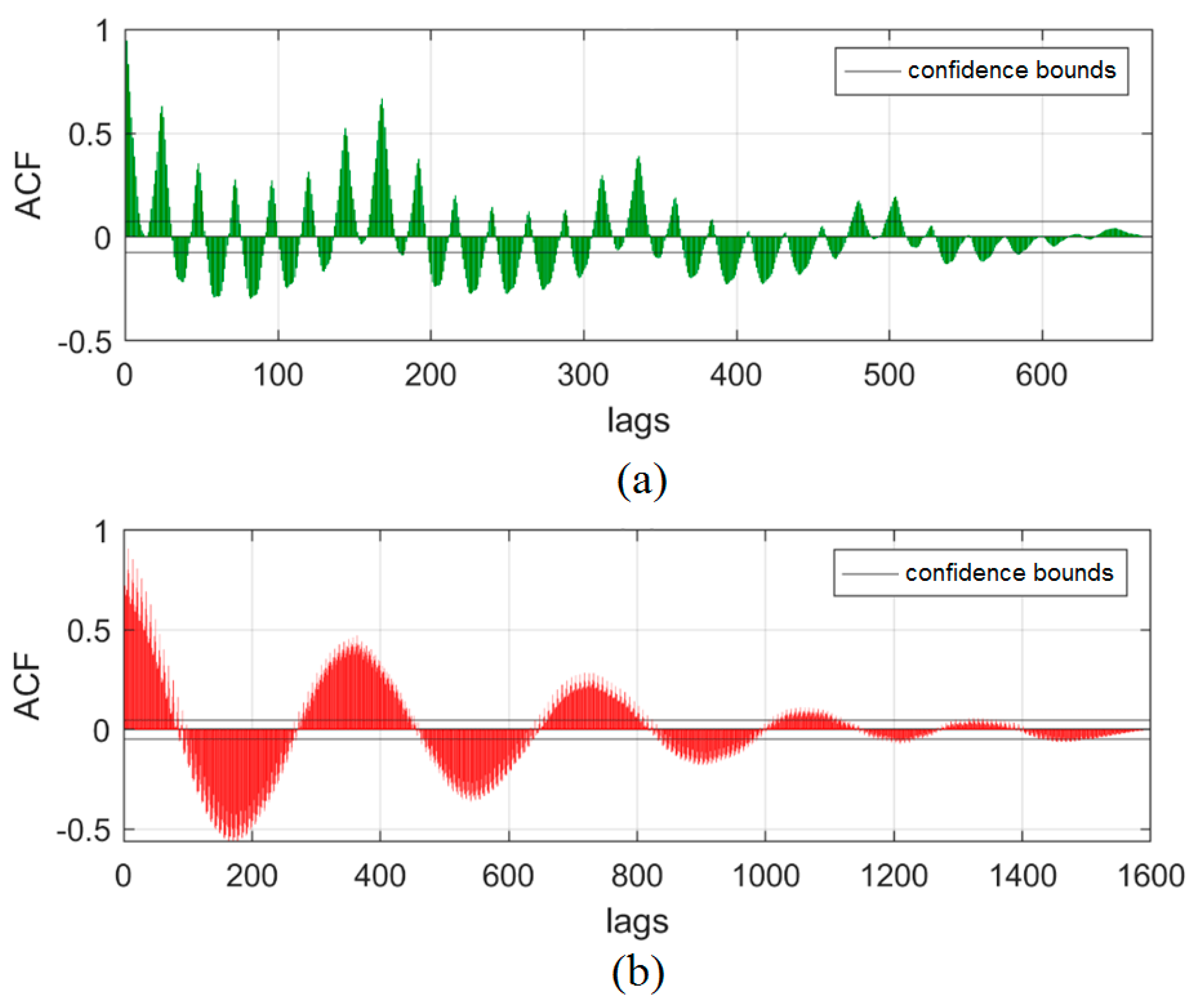
Hyperparameters are crucial to many machine learning algorithms. Conventional methods like grid search and random search can be expensive when tuning the hyperparameters of an ESN model. Recently, BOA approaches have become popular in the machine learning community as efficient tools for tuning hyperparameters. In other words, BOA can be useful to model-based approaches for automatically configuring hyperparameters to generate a surrogate model of some unknown function that would otherwise be too expensive to query in full.
Our proposal consists in evaluate Bayesian optimized ESNs for load forecasting tasks. However, hyperparameters tuning of the reservoir for ESN have a great influence on the performance of the network, so suitable values must be set for them. The training of an ESN requires the specification of basically seven hyperparameters, named: spectral radius, size of the reservoir (number of internal units), input scaling, input shift, teacher scaling, teacher shift and also feedback scaling. In our proposal, these hyperparameters are approached as decision variables to be optimized and the activation function adopted is the sigmoid function.
The hyperparameters of the ESN are optimized with BOA, each with a different kind of acquisition function for sake of comparison, which is (i) the expected improvement (EI), (ii) the probability of improvement (PI) and (iii) the lower confidence bound (LCB).
The ESNs are set with one input and one output, where the input is a sequence of load history (time series) and the output is a sequence of load predictions one-step ahead. Hence, the problem is stated as one-step ahead forecasting—that is, the forecasting horizon, also known as the prediction interval, is set to one. Data pre-processing consists of dividing by the maximum value for normalization and division into training, validation and test sets. The single feature considered is the load history one hour behind, since we expect that the echo state property reminds us of the recent history of loads that entered the reservoir.
The search space of hyperparameters are given in Table 1. The spectral radius is a positive value and must be lower than one to guarantee the echo state property, the number of internal units was empirically limited to 100 due to computational burden (the continuous value is rounded before being used), the input/teacher scales and shifts give freedom to optimize the respective normalization and operation points, and finally, the feedback scaling determines the weights of the output to the reservoir.
The cost function receives, as arguments, a set of hyperparameters, the training input, the output, the validation input, and the validation output, generates the ESN architecture, trains it with the control hyperparameter settings and returns the validation error. This process is repeated for 50 iterations for each run, with a total of 50 independent runs.

3.2. Datasets

Fortunately, electricity load data are abundant and, most of the time, public. However, to compare the performance of a proposed method it is necessary to know, beyond the data, the reported results from other publications, the approach adopted for data division in training and test sets, the forecasting horizon and the metric used for results evaluation.
The load forecasting problem may be formulated as a univariate or multivariate time series forecasting problem. Univariate problems use previous values of the time series as predictors, while multivariate problems use additional features such as weather and calendar data. Additional features may improve the performance of the prediction; however, care must be taken with collinearity and the extra effort necessary to predict weather features. For example, if a model uses temperature as an input, the evolution of predictions over time will need to feed back the predicted values as well as the unknown future temperature values that will be forecasted. In this study, the univariate load forecasting approach is adopted.
We adopt two datasets, the first is a load time series in GW (gigawatts) from Poland, also used by [14] and can be downloaded from [63], which is composed of 1601 samples, 1400 for training and 201 for testing. Since ESN explores the sequential feature of time series, cross-validation is not possible, so the validation set to be used as the cost during the optimization process is composed of the last 200 samples from the training set in a hold-out scheme.
The second dataset is from Brazil and there are no results to be used as a benchmark, so we also intend to contribute by generating a benchmark for these data, and to achieve that we followed the same strategy to deal with data as in [2]. The data selected are the hourly loads in MW from the first four weeks from the south region in Brazil; the first three weeks are for training and the test is performed over the fourth week, the validation set is drawn from the training and corresponds to the third week, also in a hold-out scheme. The Brazilian dataset can be downloaded from [64].
The dataset descriptions are exhibited in Table 2 and Figure 2. The size of the Polish time series is higher than the Brazilian dataset, but both dataset measures are regularly sampled at hourly intervals. The mean values of both datasets are quite close to the median, showing that the values are not skewed. The autocorrelation function bar charts indicate that there is a significative correlation among many past values and the current value of the time series. Considering each significative lag as an input would lead to a lot of inputs in the model and hence it would possibly cause overfitting due to the curse of dimensionality. ESNs, as any RNN, are appropriate for predicting time series because they can deal with those lags implicitly in the hidden layer, called a reservoir, through an intrinsic memory and as so they do not require each lag as a different input.

3.3. Performance Evaluation of the Forecasting

Forecast evaluation involves comparing a set of predictions with their corresponding ex-post actual values. There are a variety of error measures that can be used for assessing forecasting performances, including the mean squared error (MSE), the mean absolute error (MAE), the mean absolute percentage error (MAPE). In this paper, test results are evaluated in terms of MSE given by
M S E = 1 N i = 1 N ( y ^ i y i ) 2
where N is the number of evaluation points, y ^ is the forecasted value and y is the actual value.
If the model structure and parameter estimates obtained by the ESN are statistically valid, the system model residual should be uncorrelated with all linear and nonlinear combinations of past inputs and outputs. For nonlinear systems, under some mild assumptions, this can be tested by computing the following correlation tests proposed by [65] are calculated as
{ φ ξ ξ ( τ ) = δ ( τ ) φ u ξ ( τ ) = 0 , τ φ ξ ( ξ u ) ( τ ) = 0 , τ 0 φ ( u 2 ) ξ ( τ ) = 0 ,    τ φ ( u 2 ) ξ 2 ( τ ) = 0 ,    τ
where δ(∙) is the Kronecker delta function ( u 2 ) ( t ) = ( u ( t ) ) 2 u 2 ¯ ,   ( ξ u ) = ξ ( t + 1 ) u ( t + 1 ) , a ¯ is the mean of a and φ a b is the normalized cross-correlation given by
φ a b ( τ ) = t = 1 N τ [ a ( t ) a ¯ ] [ b ( t + τ ) b ¯ ] [ t = 1 N [ a ( t ) a ¯ ] 2 t = 1 N [ b ( t ) b ¯ ] 2 ] 1 2 ,
In practice, if these correlation functions in Equation (9) fall within the confidence intervals at a given significance level, the model is regarded as adequate and acceptable.

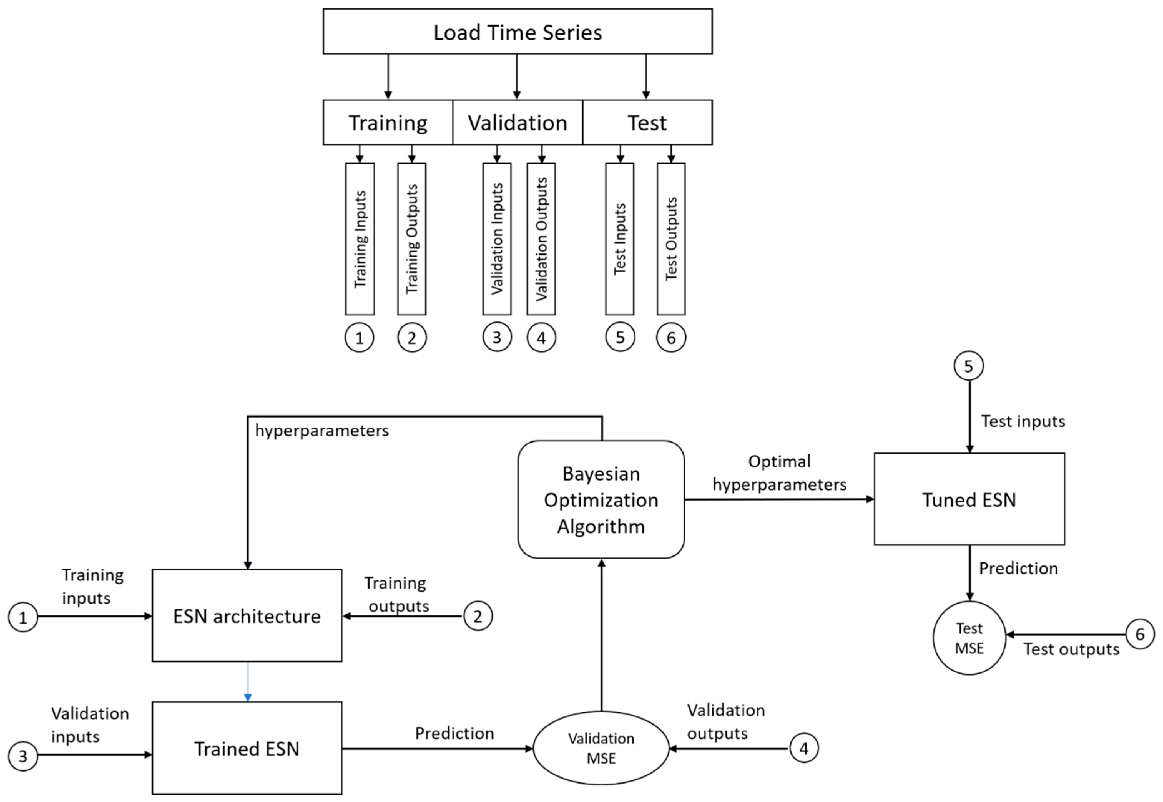
3.4. General View of the Proposed Forecasting Approach

Figure 3 presents a detailed flowchart of the proposed system. Suppose we have an initialized ESN architecture and an initial hyperparameter set. After supervised learning with training inputs and outputs, a trained ESN is achieved. Then, its predictions, given the validation set inputs, are compared with true validation outputs using the MSE, named the validation MSE. The BOA, intended to minimize the validation MSE, iteratively adjusts the hyperparameters until an optimal set of hyperparameters is found. Next, an ESN is tuned with the optimal hyperparameters and produces predictions, given the test inputs. Those predictions are compared with true test set outputs using the MSE, named the test MSE or MSE values for the test set.

4. Results and Discussion
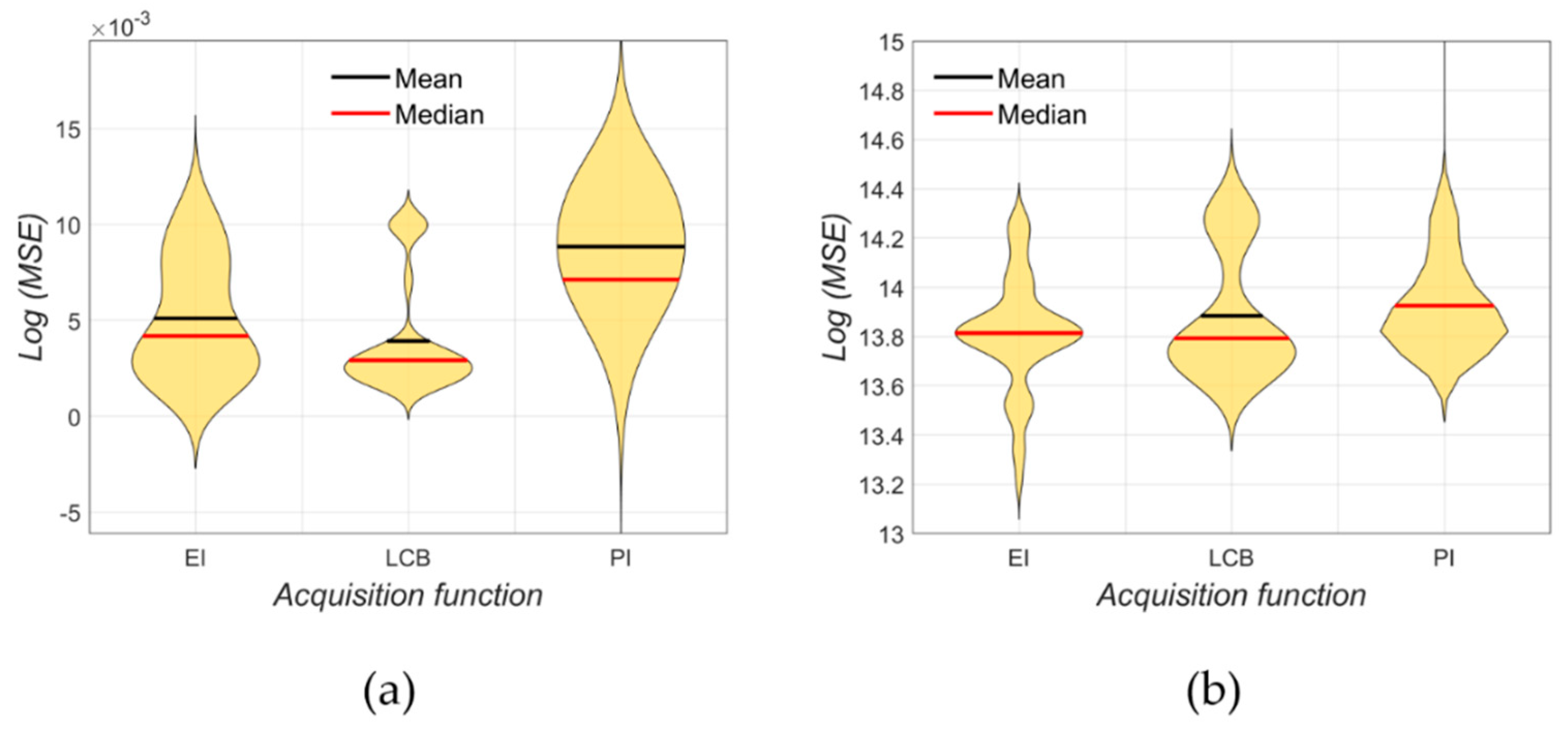
This section presents the results as well as their discussion.

4.1. Results

The optimization is performed for both datasets for 50 runs and the convergence curves of mean objective values and best objective values are analyzed for each type of acquisition function considered in the study. The MSE values of the test sets are compared (prediction versus actual data plots and correlation tests) and the best solutions are presented. The convergence analysis uses the MSE values for the validation set, while statistics descriptions and correlation tests use the MSE values for the test set.
In terms of BOA, the maximum number of iterations had to be arbitrarily set as a stopping criterion. To choose the maximum number of iterations, a single random initialization has been analyzed, increasing the maximum number of iterations in steps of 10 until any improvement had been significantly made, which has been observed after approximately 30 iterations. Due to the possibility of other initialization requirements of more iterations until convergence, this number has been arbitrarily extended to 50 for the BOA in this paper.
Since the solution of the problem is unknown, as is the case for most real-world problems, it is not possible to ensure that the probability of converging to local has been eliminated. However, multiple runs of the optimization algorithm from different starting points in the search space are expected to reduce the bias due to starting conditions. On the other side, guessing how many starting points should be enough to eliminate such bias is uncertain, and most of the time is limited by the computational effort required for each optimization run. Fifty runs are often employed in the literature regarding the comparison of algorithms in global optimization tasks.
The main performance index considered is the MSE measure over the test sets, as presented in Table 3 and Table 4. The results from [66] are included for comparison and are derived from Support Vector Regression (SVR) algorithms in the single, denoised and with Empirical Mode Decomposition (EMD) versions. The first three columns contain our results for the Expected Improvement Bayesian Optimized ESN (EI-BO-ESN), Lower Confidence Bound Bayesian Optimized ESN (LCB-BO-ESN) and Probability of Improvement Bayesian Optimized ESN (PI-BO-ESN). Optimization statistics for both datasets exhibited in Table 3 and Table 4 are graphically illustrated through violin plots in Figure 4a,b. The difference in magnitude from one dataset to another is due to the variable unit, which is in MW for Brazil and GW for Poland.
The results are evaluated in terms of statistical measures, as exhibited in Table 3 and Table 4, due to the randomness characteristic of the optimization algorithm. If a single random seed is used, it could bias the results in favor of a specific model. A method to overcome such biasing is to perform several runs of optimization and evaluate the statistical measures of central tendency and dispersion. A model that results in lower mean and median MSE values over 50 runs will probably present a lower MSE value in a new random run of the optimization.
Some features about the error distributions may be noticed from analyzing the violin plots in Figure 4a,b. For both datasets, the LCB acquisition function errors are bi-modal, with the highest mode near the median and the lowest mode near the maximum. The EI acquisition function error distribution is tailored to the minimum for the Polish dataset and symmetric for the Brazilian dataset. Conversely, the PI acquisition function error distribution is symmetric for the Polish dataset and tailored to the minimum for the Brazilian dataset. All errors are more likely to lie near the median value.
The convergence curves for the best model for Polish and Brazilian datasets are presented in Figure 5a,b, respectively (i.e., LCB-BO-ESN for the Polish dataset and EI-BO-ESN for the Brazilian dataset). Each plot contains the log of the MSE for each iteration of the optimization algorithm over the test set—more specifically, the median trend surrounded by boxplots to illustrate divergences among the runs.
Figure 6a,b exhibit the execution time behavior along with the iterations for an Intel i7-7500U 3.5 GHz processor and 20 GB RAM (Random Access Memory). The code has been implemented in the Matlab computational environment. The black line represents the median values while the shaded area represents the span between the maximum and minimum execution times of each iteration. The green line represents the cumulative execution time along with the iterations. Histograms of total execution times are shown in Figure 7a,b for the Polish and Brazilian datasets, respectively.
The frequency of values found as best hyperparameters are exhibited in Figure 8 and Figure 9 for the Polish and Brazilian datasets, respectively. Each pair of hyperparameters is compared against each other and color bars indicate the most frequency optimized values. The predictions of the LCB-BO-ESN algorithm over the test set are shown in Figure 10a for the Polish dataset and of the EI-BO-ESN in Figure 10b for the Brazilian dataset, and the correlation tests of the best predictions (i.e., LCB-BO-ESN for Polish and EI-BO-ESN for Brazilian datasets) are presented in Figure 11.

4.2. Discussion

From the Polish dataset statistics (Table 3 and Figure 4a) it is noticed that the LCB-BO-ESN achieves the lower mean and median MSE over all the runs and also the minimum MSE and the lowest maximum MSE; however, PI-BO-ESN achieves the lowest standard deviation. All ESNs improved the predictions—that is, they found the lowest minimum values compared to the SVR models.
From the Brazilian dataset statistics (Table 4 and Figure 4b), it can be observed that the EI-BO-ESN achieves the lowest mean standard deviation, minimum and maximum MSE among all the runs, however, LCB-BO-ESN achieves the lowest median MSE value. These results may now serve as a benchmark for future research.
Violin plots (Figure 4) aggregate information about central tendency and dispersion measures with a density distribution curve. The variants EI and PI present a unimodal behavior of MSE values while the LCB variant presents a bi-modality. Such a bi-modality indicates that there is a prominent occurrence of convergence to local minima when LCB variant is employed, despite it present the lowest median for both datasets. However, even when presenting the lowest median for the Brazilian dataset, its higher standard deviation and skew (deviation between the median and mean), together with the inability to find an extreme minimum value, makes EI more advantageous than LCB.
All runs converge for the same approximate value with little deviation after a certain number of iterations, which is 39 for the Polish dataset (Figure 5a) and 18 for the Brazilian dataset (Figure 5b). After the fifth iteration in the Polish dataset, a value near the minimum had already been achieved in some of the runs as shown in the lower boxplot whiskers, while in the Brazilian dataset this happened from the first iteration.
Regarding the execution times, the iteration tends to take approximately a median value two seconds after an initial transient period, presenting a slightly linear increase along with the iterations (Figure 6a,b). This linearity in time is perceived at the median cumulative time of the runs, which terminates at 100 s for the Polish dataset and 90 s for the Brazilian dataset. Most of the runs, for both datasets, take between 80 and 90 s of total execution time (Figure 7a,b) and all of them are executed in a duration ranging from 80 s (minimum) to 130 s (maximum).
Dealing with optimization on real-word datasets does not bring a known minimum value for comparison, so the best hyperparameters are grouped in pairs to get hints of its best tuning values and relationships. The Polish dataset best hyperparameters (Figure 8) suggests that an SR near one is the best choice considering an ESN with approximately 80 internal units, Tsc near one, Isc near one, Tsh near-zero or −0.5, and Ish near 0.2; however, it would be improved if it reaches around 0.7 with an Fb of 0.6. For example, improved results are also achieved with N = 60 and Isc = 0.4, as well as with Fb = 0.6 and Ish = −0.2.
In terms of the Brazilian dataset, the best hyperparameters (Figure 9), the best choices are lower N with SR = 0.6, Isc near zero with SR = 1, Ish = 0.4 with SR = 1, Tsc = 1 with SR = 1, Tsh = 0 with SR = 1, Fb = 0.3 with SR = 1, Isc near zero with lower N, Ish = −0.5 or +0.5 with lower N, Tsc = 0.7 with lower N, Tsh = −0.5 with lower N, Fb near zero with lower N, Ish = 0.4 with lower Isc, Tsc near one with Isc near zero, Tsh near zero with Isc near zero, Fb near one with Isc near zero, Tsc = 0.7 with Ish = 0.4, Tsh near zero with Ish = 0.5, Tsh = −0.5 and Tsc = 0.6, Fb = 0.2 and Tsc = 0.6, Fb = 0.2 and Tsh = 0.4.
Figure 10a,b show that the best predictions follow the nonlinear pattern of the load; in the Polish dataset, it is possible to notice the highest errors between the 60th and 100th hours, where there is a change in the mean value, and for the Brazilian dataset the highest errors are noticed during the first ten hours; however, the predictions follow the actual data. Discrepancies between predicted and actual data are due to the difficult-to-capture non-linear behavior of the time series that have not been taken into account by the model. The prediction model is trained and validated using the previous values of the time series and will generalize over these unknown values with a non-linear relationship to the previous values.
It is possible to notice that the prediction for the Polish dataset complies with all the tests in Figure 11, while the predictions for the Brazilian dataset do not comply with any. This means there may be inputs (features, load history) that are not properly echoed by the optimized ESN, meaning that perhaps it requires the use of a different activation function or even the addition of extra inputs to the network.

5. Conclusions and Future Research Direction

ESNs are an effective alternative to conventional RNNs due to their fast training process and good performance in dynamic system modeling. In this work, it has been proposed the BOA of ESN hyperparameters for load forecasting. Existing methods use a trial and error approach for the hyperparameters tuning or generates a large number of models and then apply a model selection algorithm. Results were compared with other published results and show that the proposed approach achieves similar performance when compared to the best of them; beyond that, a benchmark was proposed for the Brazilian dataset.
In terms of management implications, the adoption of forecasting models to short-term forecasting is useful. Management decisions can be made using reliable information. Hence, decisions taken by electricity suppliers and consumers will be more accurate as the load predictions are also more accurate. Some examples regarding the supplier side are about the allocation of resources such as hydric reservoir level, coal or oil stocks, and operational and maintenance planning. On the consumer side, the management of contracts that offer an incentive for non-peak load hours is more precise and the load distribution may be better with accurate forecasts.
For future research we intend to investigate the influence of other types of activation functions in the ESN, the compromise between the echo state property and the input addition, as well other variants of the BOA. Other optimization algorithms combined with chaotic sequences [67,68,69] could be applied to obtain the best hyperparameters. Besides, LSTM, gated recurrent unit (GRU), least squares-support vector regression (LS-SVR) and other promising machine learning models for time series forecasting must be included in a comparison with the ESN. Future research also intends to include a higher number of datasets with different characteristics, such as lower correlations among features and output, evaluations of the different numbers of iterations and stopping criteria for hyperparameter tuning, as well as the assessment of prediction performance for different prediction intervals.

Author Contributions

G.T.R.: Conceptualization, Methodology, Formal analysis, Validation, Writing-original draft, Writing-review & editing. J.G.S.: Conceptualization, Methodology, Formal analysis, Validation, Writing-original draft, Writing-review & editing. N.F.: Conceptualization, Methodology, Formal analysis, Validation, Writing-original draft, Writing-review & editing. V.C.M.: Conceptualization, Writing-review & editing. L.d.S.C.: Conceptualization, Writing-review & editing. All authors have read and agreed to the published version of the manuscript.

Funding

The authors would like to thank the National Council of Scientific and Technologic Development of Brazil—CNPq (Grants: 307958/2019-1-PQ, 307966/2019-4-PQ, 405101/2016-3-Univ, 404659/2016-0-Univ) and Fundação Araucária (PRONEX-FA/CNPq 042/2018) for its financial support of this work. Furthermore, the authors wish to thank the Editor and anonymous referees for their constructive comments and recommendations, which have significantly improved the presentation of this paper.

Conflicts of Interest

The authors declare no conflict of interest.

References

  1. Amarasinghe, K.; Marino, D.L.; Manic, M. Deep neural networks for energy load forecasting. In Proceedings of the 26th IEEE International Symposium on Industrial Electronics (ISIE), Edinburgh, Scotland, 19–21 June 2017; pp. 1483–1488. [Google Scholar] [CrossRef]
  2. Qiu, X.; Ren, Y.; Nagaratnam, P.; Amaratunga, G.A.J. Empirical mode decomposition based ensemble deep learning for load demand time series forecasting. Appl. Soft Comput. J. 2017, 54, 246–255. [Google Scholar] [CrossRef]
  3. Bedi, J.; Toshniwal, D. Deep learning framework to forecast electricity demand. Appl. Energy 2019, 238, 1312–1326. [Google Scholar] [CrossRef]
  4. Xiuyun, G.; Ying, W.; Yang, G.; Chengzhi, S.; Wen, X.; Yimiao, Y. Short-term load forecasting model of gru network based on deep learning framework. In Proceedings of the 2nd IEEE Conference on Energy Internet and Energy System Integration (EI2), Beijing, China, 20–22 October 2018; pp. 1–4. [Google Scholar] [CrossRef]
  5. Yudantaka, K.; Kim, J.S.; Song, H. Dual deep learning networks based load forecasting with partial real-time information and its application to system marginal price prediction. Energies 2019, 13, 148. [Google Scholar] [CrossRef] [Green Version]
  6. Shi, T.; Mei, F.; Lu, J.; Pan, Y.; Zhou, C.; Wu, J.; Zheng, J. Phase space reconstruction algorithm and deep learning-based very short-term bus load forecasting. Energies 2019, 12, 4349. [Google Scholar] [CrossRef] [Green Version]
  7. Ribeiro, G.T.; Gritti, M.C.; Ayala, H.V.; Mariani, V.C.; Coelho, L.S. Short-term load forecasting using wavenet ensemble approaches. In Proceedings of the 2016 International Joint Conference on Neural Networks (IJCNN), Vancouver, BC, Canada, 24–29 July 2016; pp. 727–734. [Google Scholar] [CrossRef]
  8. Li, S.; Wang, P.; Goel, L. A Novel wavelet-based ensemble method for short-term load forecasting with hybrid neural networks and feature selection. IEEE Trans. Power Syst. 2016, 31, 1788–1798. [Google Scholar] [CrossRef]
  9. Chen, L.; Chiang, H.; Dong, N.; Liu, R. Group-based chaos genetic algorithm and non-linear ensemble of neural networks for short-term load forecasting. IET Gener. Transm. Distrib. 2016, 10, 1440–1447. [Google Scholar] [CrossRef]
  10. Nowotarski, J.; Liu, B.; Weron, R.; Hong, T. Improving short term load forecast accuracy via combining sister forecasts. Energy 2016, 98, 40–49. [Google Scholar] [CrossRef]
  11. Hassan, S.; Khosravi, A.; Jaafar, J. Examining performance of aggregation algorithms for neural network-based electricity demand forecasting. Int. J. Electr. Power Energy Syst. 2015, 64, 1098–1105. [Google Scholar] [CrossRef]
  12. Khwaja, A.S.; Naeem, M.; Anpalagan, A.; Venetsanopoulos, A.; Venkatesh, B. Improved short-term load forecasting using bagged neural networks. Electr. Power Syst. Res. 2015, 125, 109–115. [Google Scholar] [CrossRef]
  13. Khuntia, S.R.; Rueda, J.L.; van der Meijden, M.A.M.M. Neural network-based load forecasting and error implication for short-term horizon. In Proceedings of the International Joint Conference on Neural Networks (IJCNN), Vancouver, BC, Canada, 24–29 July 2016; pp. 4970–4975. [Google Scholar] [CrossRef]
  14. Dudek, G. Neural networks for pattern-based short-term load forecasting: A comparative study. Neurocomputing 2016, 205, 64–74. [Google Scholar] [CrossRef]
  15. Rana, M.; Koprinska, I. Forecasting electricity load with advanced wavelet neural networks. Neurocomputing 2016, 182, 118–132. [Google Scholar] [CrossRef]
  16. Zjavka, L. Short-term power demand forecasting using the differential polynomial neural network. Int. J. Comput. Intell. Syst. 2014, 8, 297–306. [Google Scholar] [CrossRef] [Green Version]
  17. Li, L.-L.; Sun, J.; Wang, C.-H.; Zhou, Y.-T.; Lin, K.-P. Enhanced Gaussian process mixture model for short-term electric load forecasting. Inf. Sci. 2019, 477, 386–398. [Google Scholar] [CrossRef]
  18. Muzaffar, S.; Afshari, A. Short-term load forecasts using LSTM networks. Energy Procedia 2019, 158, 2922–2927. [Google Scholar] [CrossRef]
  19. Wang, S.; Wang, X.; Wang, S.; Wang, D. Bi-directional long short-term memory method based on attention mechanism and rolling update for short-term load forecasting. Int. J. Electr. Power Energy Syst. 2019, 109, 470–479. [Google Scholar] [CrossRef]
  20. Wang, X.; Fang, F.; Zhang, X.; Liu, Y.; Wei, L.; Shi, Y. LSTM-based Short-term Load Forecasting for Building Electricity Consumption. In Proceedings of the IEEE 28th International Symposium on Industrial Electronics (ISIE), Vancouver, BC, Canada, 24–29 July 2019; pp. 1418–1423. [Google Scholar] [CrossRef]
  21. Kong, W.; Dong, Z.Y.; Jia, Y.; Hill, D.J.; Xu, Y.; Zhang, Y. Short-term residential load forecasting based on LSTM recurrent neural network. IEEE Trans. Smart Grid 2019, 10, 841–851. [Google Scholar] [CrossRef]
  22. Bouktif, S.; Fiaz, A.; Ouni, A.; Serhani, M.A. Multi-sequence LSTM-RNN deep learning and metaheuristics for electric load forecasting. Energies 2020, 13, 391. [Google Scholar] [CrossRef] [Green Version]
  23. Dedinec, A.; Filiposka, S.; Dedinec, A.; Kocarev, L. Deep belief network based electricity load forecasting: An analysis of Macedonian case. Energy 2016, 115, 1688–1700. [Google Scholar] [CrossRef]
  24. Ouyang, T.; He, Y.; Li, H.; Sun, Z.; Baek, S. Modeling and forecasting short-term power load with copula model and deep belief network. IEEE Trans. Emerg. Top. Comput. Intell. 2019, 3, 127–136. [Google Scholar] [CrossRef] [Green Version]
  25. Dudek, G. Heterogeneous ensembles for short-term electricity demand forecasting. In Proceedings of the 17th International Scientific Conference on Electric Power Engineering (EPE), Prague, Czech Republic, 16–18 May 2016; pp. 1–6. [Google Scholar] [CrossRef]
  26. Barak, S.; Sadegh, S.S. Forecasting energy consumption using ensemble ARIMA–ANFIS hybrid algorithm. Int. J. Electr. Power Energy Syst. 2016, 82, 92–104. [Google Scholar] [CrossRef] [Green Version]
  27. Burger, E.M.; Moura, S.J. Gated ensemble learning method for demand-side electricity load forecasting. Energy Build. 2015, 109, 23–34. [Google Scholar] [CrossRef]
  28. Shen, W.; Babushkin, V.; Aung, Z.; Woon, W.L. An ensemble model for day-ahead electricity demand time series forecasting. In Proceedings of the 4th International Conference on Future Energy Systems (e-Energy ’13); ACM Press: New York, NY, USA, 2013; pp. 51–62. [Google Scholar] [CrossRef]
  29. Zhang, R.; Xu, Y.; Dong, Z.Y.; Kong, W.; Wong, K.P. A composite k-nearest neighbor model for day-ahead load forecasting with limited temperature forecasts. In Proceedings of the IEEE Power and Energy Society General Meeting (PESGM), Boston, MA, USA, 17–21 July 2016; pp. 1–5. [Google Scholar] [CrossRef]
  30. Bianchi, F.M.; De Santis, E.; Rizzi, A.; Sadeghian, A. Short-term electric load forecasting using echo state networks and PCA decomposition. IEEE Access 2015, 3, 1931–1943. [Google Scholar] [CrossRef]
  31. Wang, Z.; Zeng, Y.R.; Wang, S.; Wang, L. Optimizing echo state network with backtracking search optimization algorithm for time series forecasting. Eng. Appl. Artif. Intell. 2019, 81, 117–132. [Google Scholar] [CrossRef]
  32. Ma, Q.; Shen, L.; Cottrell, G.W. DeePr-ESN: A deep projection-encoding echo-state network. Inf. Sci. (Ny). 2020, 511, 152–171. [Google Scholar] [CrossRef]
  33. McDermott, P.L.; Wikle, C.K. Deep echo state networks with uncertainty quantification for spatio-temporal forecasting. Environmetrics 2019, 30, e2553. [Google Scholar] [CrossRef] [Green Version]
  34. Hu, H.; Wang, L.; Peng, L.; Zeng, Y.R. Effective energy consumption forecasting using enhanced bagged echo state network. Energy 2020, 193. [Google Scholar] [CrossRef]
  35. Li, Z.; Liu, X.; Chen, L. Load interval forecasting methods based on an ensemble of Extreme Learning Machines. In Proceedings of the IEEE Power & Energy Society General Meeting, Denver, CO, USA, 26–30 July 2015; IEEE: Denver, CO, USA, 2015; pp. 1–5. [Google Scholar] [CrossRef]
  36. Xu, Y.; Dong, Z.Y.; Meng, K.; Wong, K.P.; Zhang, R. Short-term load forecasting of Australian National Electricity Market by an ensemble model of extreme learning machine. IET Gener. Transm. Distrib. 2013, 7, 391–397. [Google Scholar] [CrossRef]
  37. Papadopoulos, S.; Karakatsanis, I. Short-term electricity load forecasting using time series and ensemble learning methods. In Proceedings of the IEEE Power and Energy Conference at Illinois (PECI), Champaign, IL, USA, 20–21 Feburary 2015; pp. 1–6. [Google Scholar] [CrossRef]
  38. Nadtoka, I.I.; Balasim, M.A.-Z. Mathematical modelling and short-term forecasting of electricity consumption of the power system, with due account of air temperature and natural illumination, based on support vector machine and particle swarm. Procedia Eng. 2015, 129, 657–663. [Google Scholar] [CrossRef] [Green Version]
  39. Kumaran, J.; Ravi, G. Long-term sector-wise electrical energy forecasting using artificial neural network and biogeography-based optimization. Electr. Power Components Syst. 2015, 43, 1225–1235. [Google Scholar] [CrossRef]
  40. Kavousi-Fard, A. A new fuzzy-based feature selection and hybrid TLA–ANN modelling for short-term load forecasting. J. Exp. Theor. Artif. Intell. 2013, 25, 543–557. [Google Scholar] [CrossRef]
  41. Singh, P.; Dwivedi, P. A novel hybrid model based on neural network and multi-objective optimization for effective load forecast. Energy 2019, 182, 606–622. [Google Scholar] [CrossRef]
  42. Bento, P.M.R.; Pombo, J.A.N.; Calado, M.R.A.; Mariano, S.J.P.S. Optimization of neural network with wavelet transform and improved data selection using bat algorithm for short-term load forecasting. Neurocomputing 2019, 358, 53–71. [Google Scholar] [CrossRef]
  43. Singh, P.; Dwivedi, P. Integration of new evolutionary approach with artificial neural network for solving short term load forecast problem. Appl. Energy 2018, 217, 537–549. [Google Scholar] [CrossRef]
  44. Raza, M.Q.; Khosravi, A. A review on artificial intelligence based load demand forecasting techniques for smart grid and buildings. Renew. Sustain. Energy Rev. 2015, 50, 1352–1372. [Google Scholar] [CrossRef]
  45. Hernandez, L.; Baladron, C.; Aguiar, J.M.; Carro, B.; Sanchez-Esguevillas, A.J.; Lloret, J.; Massana, J. A survey on electric power demand forecasting: Future trends in smart grids, microgrids and smart buildings. Commun. Surv. Tutorials IEEE 2014, 16, 1460–1495. [Google Scholar] [CrossRef]
  46. Tüfekci, P. Prediction of full load electrical power output of a base load operated combined cycle power plant using machine learning methods. Int. J. Electr. Power Energy Syst. 2014, 60, 126–140. [Google Scholar] [CrossRef]
  47. Matijaš, M.; Suykens, J.A.K.; Krajcar, S. Load forecasting using a multivariate meta-learning system. Expert Syst. Appl. 2013, 40, 4427–4437. [Google Scholar] [CrossRef] [Green Version]
  48. DING, Y. Data Science for Wind Energy; CRC Press: Boca Raton, FL, USA, 2019; ISBN 9781138590526. [Google Scholar]
  49. Liu, Y.; Zhao, J.; Wang, W. A Gaussian process echo state networks model for time series forecasting. In Proceedings of the Joint IFSA World Congress and NAFIPS Annual Meeting (IFSA/NAFIPS), Edmonton, AB, Canada, 24–28 June 2013; IEEE: Edmonton, AB, Canada, 2013; pp. 643–648. [Google Scholar] [CrossRef]
  50. Velasco Rueda, C. EsnPredictor: Ferramenta de Previsão de Séries Temporais Baseada em Echo State Networks Otimizada por Algoritmos Genéticos e Particle Swarm Optimization; Pontifícia Universidade Católica do Rio de Janeiro: Rio de Janeiro, Brazil, 2014; (In Portuguese). [Google Scholar] [CrossRef]
  51. Liu, C.; Zhang, H.; Yao, X.; Zhang, K. Echo state networks with double-reservoir for time-series prediction. In Proceedings of the 7th International Conference on Intelligent Control and Information Processing (ICICIP), Siem Reap, Cambodia, 1–4 December 2016; pp. 196–202. [Google Scholar] [CrossRef]
  52. López, E.; Valle, C.; Allende, H.; Gil, E.; Madsen, H. Wind power forecasting based on echo state networks and long short-term memory. Energies 2018, 11, 526. [Google Scholar] [CrossRef] [Green Version]
  53. Gouveia, H.T.V.; De Aquino, R.R.B.; Ferreira, A.A. Enhancing short-term wind power forecasting through multiresolution analysis and echo state networks. Energies 2018, 11, 824. [Google Scholar] [CrossRef] [Green Version]
  54. López, M.; Sans, C.; Valero, S.; Senabre, C. Empirical comparison of neural network and auto-regressive models in short-term load forecasting. Energies 2018, 11, 2080. [Google Scholar] [CrossRef] [Green Version]
  55. Luy, M.; Ates, V.; Barisci, N.; Polat, H.; Cam, E. Short-term fuzzy load forecasting model using genetic–fuzzy and ant colony–fuzzy knowledge base optimization. Appl. Sci. 2018, 8, 864. [Google Scholar] [CrossRef] [Green Version]
  56. Siqueira, H.; Boccato, L.; Attux, R.; Lyra, C. Unorganized machines for seasonal streamflow series forecasting. Int. J. Neural Syst. 2014, 24, 1–6. [Google Scholar] [CrossRef] [PubMed]
  57. Li, G.; Li, B.J.; Yu, X.G.; Cheng, C.T. Echo state network with Bayesian regularization for forecasting short-term power production of small hydropower plants. Energies 2015, 8, 12228–12241. [Google Scholar] [CrossRef] [Green Version]
  58. Han, M.; Mu, D. Multi-reservoir echo state network with sparse Bayesian learning. In Lecture Notes in Computer Science (Including Subseries Lecture Notes in Artificial Intelligence and Lecture Notes in Bioinformatics); Springer: Berlin/Heidelberg, Germany, 2010; pp. 450–456. [Google Scholar]
  59. Shutin, D.; Zechner, C.; Kulkarni, S.R.; Poor, H.V. Regularized variational bayesian learning of echo state networks with delay&sum readout. Neural Comput. 2012, 24, 967–995. [Google Scholar] [PubMed]
  60. Zechner, C.; Shutin, D. Bayesian learning of echo state networks with tunable filters and delay& sum readouts. In Proceedings of the IEEE International Conference on Acoustics, Speech and Signal Processing, Dallas, TX, USA , 14–19 March 2010 ; IEEE: Dallas, TX, USA, 2010; pp. 1998–2001. [Google Scholar] [CrossRef]
  61. Cerina, L.; Franco, G.; Santambrogio, M.D. Lightweight autonomous bayesian optimization of Echo-State Networks. In Proceedings of the ESANN 2019 Proceedings, 27th European Symposium on Artificial Neural Networks, Computational Intelligence and Machine Learning, Bruges, Belgium, 24–26 April 2019; pp. 637–642. [Google Scholar]
  62. Jaeger, H. The “Echo State” Approach to Analysing and Training Recurrent Neural Networks-with an Erratum Note 1; GMD Technical Report 148; German National Research Center for Information Technology: Bonn, Germany, 2010. [Google Scholar]
  63. Aalto University—Applications of Machine Learning Group Home Page. Available online: https://research.cs.aalto.fi/aml/datasets.shtml (accessed on 6 May 2020).
  64. Operador Nacional do Sistema elétrico—ONS Home Page. Available online: http://www.ons.org.br/Paginas/resultados-da-operacao/historico-da-operacao/curva_carga_horaria.aspx (accessed on 6 May 2020).
  65. Billings, S.A. Nonlinear System Identification; John Wiley & Sons, Ltd.: Chichester, UK, 2013; ISBN 9781119943594. [Google Scholar]
  66. Yaslan, Y.; Bican, B. Empirical mode decomposition based denoising method with support vector regression for time series prediction: A case study for electricity load forecasting. Measurement 2017, 103, 52–61. [Google Scholar] [CrossRef]
  67. Coelho, L.S.; Mariani, V.C.; Guerra, F.A.; da Luz, M.V.F.; Leite, J.V. Multiobjective optimization of transformer design using a chaotic evolutionary approach. IEEE Trans. Magn. 2014, 50, 669–672. [Google Scholar] [CrossRef]
  68. Coelho, L.S.; Ayala, C.H.; Mariani, V.C. A self-adaptive chaotic differential evolution algorithm using gamma distribution for unconstrained global optimization. Appl. Math. Comput. 2014, 23415, 452–459. [Google Scholar] [CrossRef]
  69. Santos, G.S.; Luvizotto, L.G.J.; Mariani, V.C.; Coelho, L.S. Least squares support vector machines with tuning based on chaotic differential evolution approach applied to the identification of a thermal process. Expert Syst. Appl. 2012, 39, 4805–4812. [Google Scholar] [CrossRef]
Figure 1. Architecture of an ESN composed of one input unit, three internal units, and one output unit for demonstration purposes: (a) description of elementary units; (b) internal weights; (c) reservoir interconnection weights; (d) reservoir intra-connection weights; (e) output weights; and (f) feedback weights. The sub-index notations mean the unit number, for example: u 1 the input unit number one, f 3 the internal unit number three, x 2 the state of internal unit number two, and y 1 the output unit number one.
Energies 13 02390 g001
Figure 2. Autocorrelation functions (ACF) bar plot with the confidence bounds for (a) the Brazilian and (b) the Polish dataset.
Energies 13 02390 g002
Figure 3. The general framework of the proposed forecasting approach based on ESN with Bayesian optimization (BO).
Energies 13 02390 g003
Figure 4. Violin plot of MSE values in log scale after 50 runs of BOA for each acquisition function in optimizing an ESN for (a) the Polish dataset, and (b) the Brazilian dataset.
Energies 13 02390 g004
Figure 5. Convergence curve for the (a) Polish dataset errors using LCB-BO and (b) Brazilian dataset errors using EI-BO, optimized ESN. The trend line is the median value, while the boxplots show the quantiles over the 50 runs.
Energies 13 02390 g005
Figure 6. Execution time for the (a) Polish dataset errors using LCB-BO and (b) Brazilian dataset errors using EI-BO optimized ESN. The black trend line and shaded area are related to the left axis, while the green line represents the cumulative execution time along iterations referred to the right axis scale.
Energies 13 02390 g006
Figure 7. Total execution time for the (a) Polish dataset errors using LCB-BO and (b) Brazilian dataset errors using EI-BO optimized ESN.
Energies 13 02390 g007
Figure 8. Best hyperparameters frequency for the Polish dataset errors using LCB-BO optimized ESN.
Energies 13 02390 g008
Figure 9. Best hyperparameters frequency for the Brazilian dataset errors using EI-BO optimized ESN.
Energies 13 02390 g009
Figure 10. Visualization of predictions (dashed) over actual (continuous) values for the (a) Polish and (b) Brazilian test sets.
Energies 13 02390 g010
Figure 11. Correlation tests for (a) Polish dataset and (b) Brazilian dataset.
Energies 13 02390 g011
Table 1. Search space of the ESN hyperparameters.
HyperparameterLower BoundUpper Bound
Spectral radius (SR)0.100.99
Internal units (N)1100
Input scaling (Isc)0.011
Input shift (Ish)−0.50.5
Teacher scaling (Tsc)0.011
Teacher shift (Tsh)−0.50.5
Feedback scaling (Fb)01
Table 2. Datasets description through statistics.
Descriptive StatisticsBrazilian DatasetPolish Dataset
Number of samples6721601
Sample interval1 h1 h
Mean11,880 MW0.96601 GW
Standard deviation1953.50 MW0.16394 GW
Minimum6949.90 MW0,6181 GW
First quartile10,413 MW0.83669 GW
Median11,773 MW0.95184 GW
Third quartile13,384 MW1.1156 GW
Maximum16,429 MW1.349 GW
Table 3. Statistical measures over best fit mean squared error (MSE) values found over the 50 runs on the Polish dataset.
Statistical MeasureEI-BO-ESNLCB-BO-ESNPI-BO-ESNSingle SVRDenoised SVREMD SVR
Mean0.00510.0039 10.0088
Median0.00420.0029 10.0071
Std0.00300.00290.0026 1
Min0.00190.0017 10.00200.00480.00470.0027
Max0.01100.0100 10.0115
1 Best value.
Table 4. Statistical measures of best fit MSE values found over the 50 runs on the Brazilian dataset.
Statistical MeasureEI-BO-ESNLCB-BO-ESNPI-BO-ESN
Mean1.02 × 10 6 11.11 × 10 6 8.78 × 10 8
Median9.99 × 10 5 9.77 × 10 5 11.12 × 10 6
Standard deviation2.31 × 10 5 12.99 × 10 5 1.68 × 10 9
Minimum5.51 × 10 5 18.46 × 10 5 9.30 × 10 5
Maximum1.57 × 10 6 11.68 × 10 6 4.81 × 10 9
1 Best value.

