An Algorithm for Recognition of Fault Conditions in the Utility Grid with Renewable Energy Penetration

Abstract

Penetration level of renewable energy (RE) in the utility grid is continuously increasing to minimize the environmental concerns, risk of energy security, and depletion of fossil fuels. The uncertain nature and availability of RE power for a short duration have created problems related to the protection, grid security, power reliability, and power quality. Further, integration of RE sources near the load centers has also pronounced the protection issues, such as false tripping, delayed tripping, etc. Hence, this paper introduces a hybrid grid protection scheme (HGPS) for the protection of the grid with RE integration. This combines the merits of the Stockwell Transform, Hilbert Transform, and Alienation Coefficient to improve performance of the protection scheme. The Stockwell Transform-based Median and Summation Index (SMSI) utilizing current signals, Hilbert Transform-based derivative index (HDI) utilizing voltage signals, and Alienation Coefficient index (ACI) utilizing voltage signals were used to compute a proposed Stockwell Transform-, Hilbert Transform-, and Alienation-based fault index (SAHFI). This SAHFI was used to recognize the fault conditions. The fault conditions were categorized using the number of faulty phases and the proposed Stockwell Transform and Hilbert Transform-based ground fault index (SHGFI) utilizing zero sequence currents. The fault conditions, such as phase and ground (PGF), any two phases (TPF), any two phases and ground (TPGF), all three phases (ATPF), and all three phases and ground (ATPGF), were recognized effectively, using the proposed SAHFI. The proposed method has the following merits: performance is least affected by the noise, it is effective in recognizing fault conditions in minimum time, and it is also effective in recognizing the fault conditions in different scenarios of the grid. Performance of the proposed approach was found to be superior compared to the discrete wavelet transform (DWT)-based method reported in the literature. The study was performed using the hybrid grid test system realized by integrating wind and solar photovoltaic (PV) plants to the IEEE-13 nodes network in MATLAB software.

1. Introduction

Capability of the renewable energy (RE) sources to meet the growing demand of electrical power has led to the increased penetration level of these sources in the network of utilities in recent years [1]. This has presented technical challenges to the power system operators and planners in terms of frequency variations, voltage regulations, efficiency, power quality (PQ) issues, grid stability issues, power reliability, and protection issues [2]. The protection challenges are due to the conversion of passive traditional feeders into active ones by the use of RE sources near load centers. Protection challenges are also observed due to reduction in the number of radial feeders and increased use of multi-tapped transmission and distribution lines for integrating RE sources and simultaneously feeding the loads [3]. A detailed study of the protection schemes and protection challenges in the power system with high penetration level of RE sources is reported in Reference [4,5,6]. The central part of the protection scheme is the detection and classification of fault conditions. Signal processing, artificial intelligence, and machine learning techniques play important role in detection and classification of the fault conditions [7]. An algorithm for detection and classification of faults in the presence of RE generation using combined use of wavelet singular entropy (WSE) and fuzzy logic (FL) is reported in Reference [8]. This is effective in identifying the faults in a time duration of 10 ms after fault inception and differentiate the fault conditions from islanding events in the presence of RE sources. A fault recognition method using a fault index (FI) computed using the detailed coefficients obtained by the decomposition of current signals is proposed in Reference [9]. Application of this method for recognition of faults in the presence of wind generation by the use of FI computed using the detail coefficient at first decomposition level of current signals using DWT is reported in Reference [10]. Application of the approach for recognition of faults in the presence of solar energy is reported in Reference [11]. Performance of this DWT-based method is affected by noise, fault recognition time is high, and range of variation of peak values of FI is large, which may generate false tripping commands during the operational events. A method for identification of faults in a utility grid when a solar photovoltaic (PV) plant is integrated and based on the use of wavelet multi-resolution singular spectrum entropy (WMRSSE) and Support Vector Machine (SVM) is reported in Reference [12]. This method is effective in recognizing the different fault conditions at fast rate in the presence of solar PV generation. In Reference [13], authors proposed a method using the Machine Learning approach for tracing of the fault current for recognizing the fault conditions in distribution systems in the presence of distributed energy resources (DER). This overcomes the demerits of the artificial intelligent (AI)- and SVM-based methods. Chen et al. [14] introduced an effective scheme for protection of a micro-grid in grid-connected mode by recognizing the fault conditions using wavelet energy and fuzzy neural network. In Reference [15], authors introduced a fuzzy-supported intelligent technique to detect and classify the fault conditions on distribution power lines where RE sources are integrated. This method is effective in recognizing the fault conditions in a time duration between quarter cycle to one cycle. A multi-class adaptive neuro-fuzzy classifier (MC-NFC) is introduced in Reference [16] to recognize the fault conditions in the presence of solar PV generation. It is established that MC-NFC has better fault classification accuracy compared to the artificial neural network (ANN) classifier. A protection scheme using the alienation coefficient and Wigner distribution function is proposed for identification of faults based on the features of current and voltage signals in the presence of solar energy [17] and both solar and wind energy [18]. This algorithm is effective to recognize faults with high penetration level of RE even in the presence of high noise level in a duration less than quarter cycle period. This article presents a method for recognition of fault conditions in the presence of renewable energy generation in addition to the conventional generation and loads. This method overcomes the demerits of the above discussed protection approaches. Hence, the main contribution of this article can be summarized by the following points:

• This article introduced a fault recognition approach that can be used for the protection of the grid with RE penetration.
• This protection scheme uses a fault index based on the features of voltage and currents extracted using the Stockwell Transform, Hilbert Transform, and Alienation Coefficient.
• This approach has the merits that its performance is least affected by noise, recognizes fault conditions in minimum time, effectively recognizes the fault conditions in different scenarios of the grid, and is free from generation of the false tripping command.
• Proposed approach effectively identify the faults using the number of faulty phases and the proposed Stockwell and Hilbert Transform-based ground fault index.

The article is structured in nine sections. The first section details the introductory part, including research gaps and contribution. The second section is related to the description of hybrid grid test system. In Section 3, protection algorithm is discussed and different proposed indexes are described. Results of simulation for recognition of fault conditions are detailed under Section 4. The fifth section describes the categorization of fault conditions, while the sixth section describes the results for various cases of study. The application of the proposed protection approach to differentiate switching transients is discussed under Section 7. A comparative study is incorporated under Section 8. Lastly, the conclusions are discussed under Section 9.

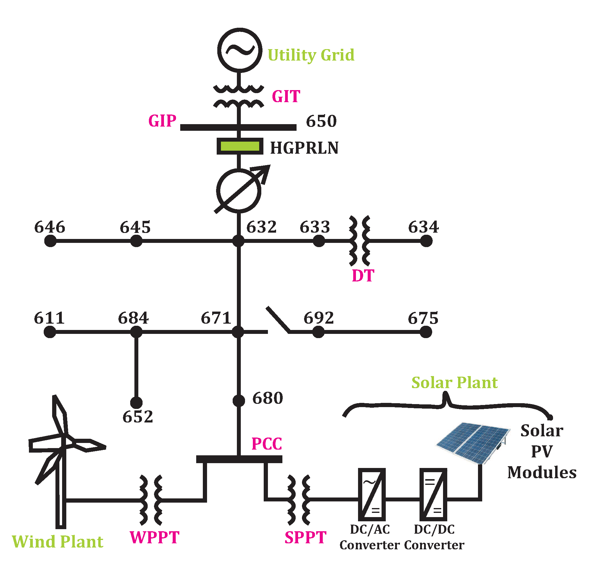
2. Proposed Test System

A hybrid grid test system (HGTS) is realized using the standard distribution network of IEEE-13 nodes and described in Figure 1. This HGTS has capacity of 5 MVA at frequency of 60 Hz and voltage levels of $0.48$ kV and $4.16$ kV. The node 634 is rated at voltage level of $0.48$ kV and the rest of the nodes are rated at $4.16$ kV. This test system is integrated to the utility grid rated at voltage level of 115 kV using a grid integration transformer (GIT) at node 650, which is considered as grid integration point (GIP). Loads with both the balanced and unbalanced nature are integrated to this grid [19,20]. A solar PV plant (SPP) of capacity 1 MW and output voltage level of 260 V is integrated on node 680 using a transformer, which is designated as SPPT. The SPP is designed using the single diode equivalent circuit of the solar cell using the modeling and data reported in Reference [21,22,23]. A wind power plant (WPP) of capacity $1.5$ MW and output voltage level of 575 V is integrated on node 680 using a transformer, which is designated as WPPT. The WPP is designed using the modeling and data reported in Reference [24,25]. The node 680 is considered as the point of common coupling (PCC) for integration of RE plants. The current and voltage measurements are performed at node 650, where the proposed protection scheme is proposed to be installed. Hence, this node is also considered as hybrid grid protection relay location node (HGPRLN) in addition to the GIP. The fault conditions are realized on the node 675, which is considered as fault condition node (FCN). A distribution transformer (DT) is connected between the nodes 634 and 633 to maintain these nodes at different voltage levels. A description of the transformers used in the proposed HGTS is provided in

Table 1. Description of the transformers. FW = first winding; SW = second winding; MVA = mega volt ampere.

Transformer	MVA	kV	kV	First Winding		Second Winding
		FW	SW	R $(\mathbf{\Omega })$	X $(\mathbf{\Omega })$	R $(\mathbf{\Omega })$	X $(\mathbf{\Omega })$
GIT	10	115.00	4.16	29.090	211.60	0.1145	0.8308
DT	5	4.16	0.48	0.3807	2.7689	0.0511	0.0042
SPPT	1	4.16	0.260	0.1730	195.70	0.0008	0.7645
WPPT	5	4.16	0.575	0.3807	2.7688	0.0510	0.0042

, where the ratings, voltage levels, resistance, and reactance of the first winding (FW) and second winding (SW) of the transformers are provided. The load data, capacitor data, and feeder data reported in Reference [26,27] are used in the proposed study.

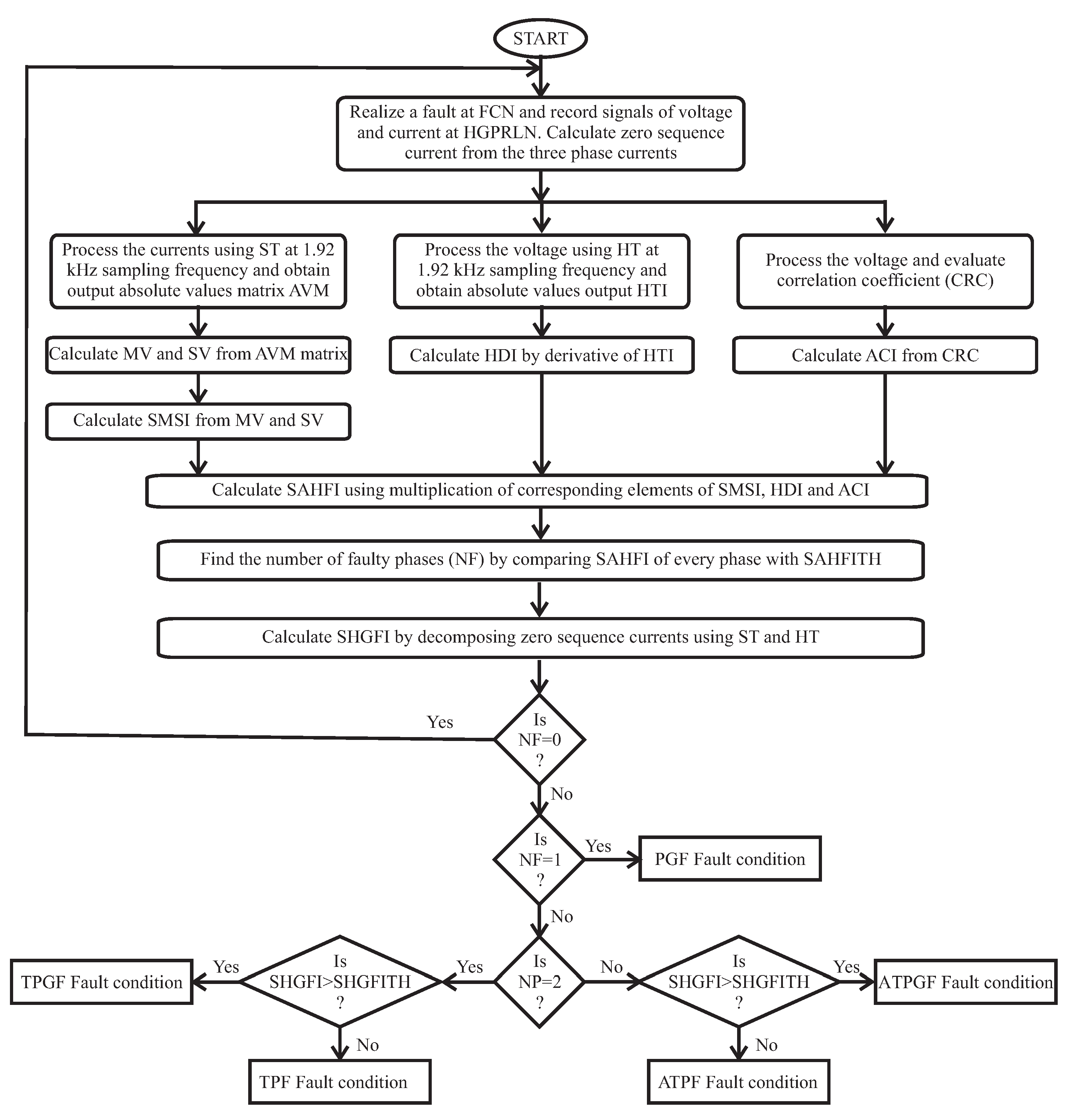
3. Protection Algorithm

The hybrid grid protection scheme (HGPS) for protection of the grid with RE integration introduced in this study is designed with five stages. The first stage calculates the Stockwell Transform based Median and Summation Index (SMSI) using the current signals. The second stage calculates the Hilbert Transform based derivative index (HDI) using the voltage signals. In third stage, Alienation Coefficient index (ACI) is computed using the voltage signals. In the fourth stage, the proposed Stockwell Transform-, Hilbert Transform-, and Alienation-based fault index (SAHFI) is computed using the SMSI, HDI, and ACI. In the fifth stage, different fault conditions are categorized using the number of faulty phases and the proposed Stockwell Transform- and Hilbert Transform-based ground fault index (SHGFI). All the stages of the proposed approach for fault recognition are detailed in Figure 2. A detailed description of the proposed indexes is provided in the following subsections.

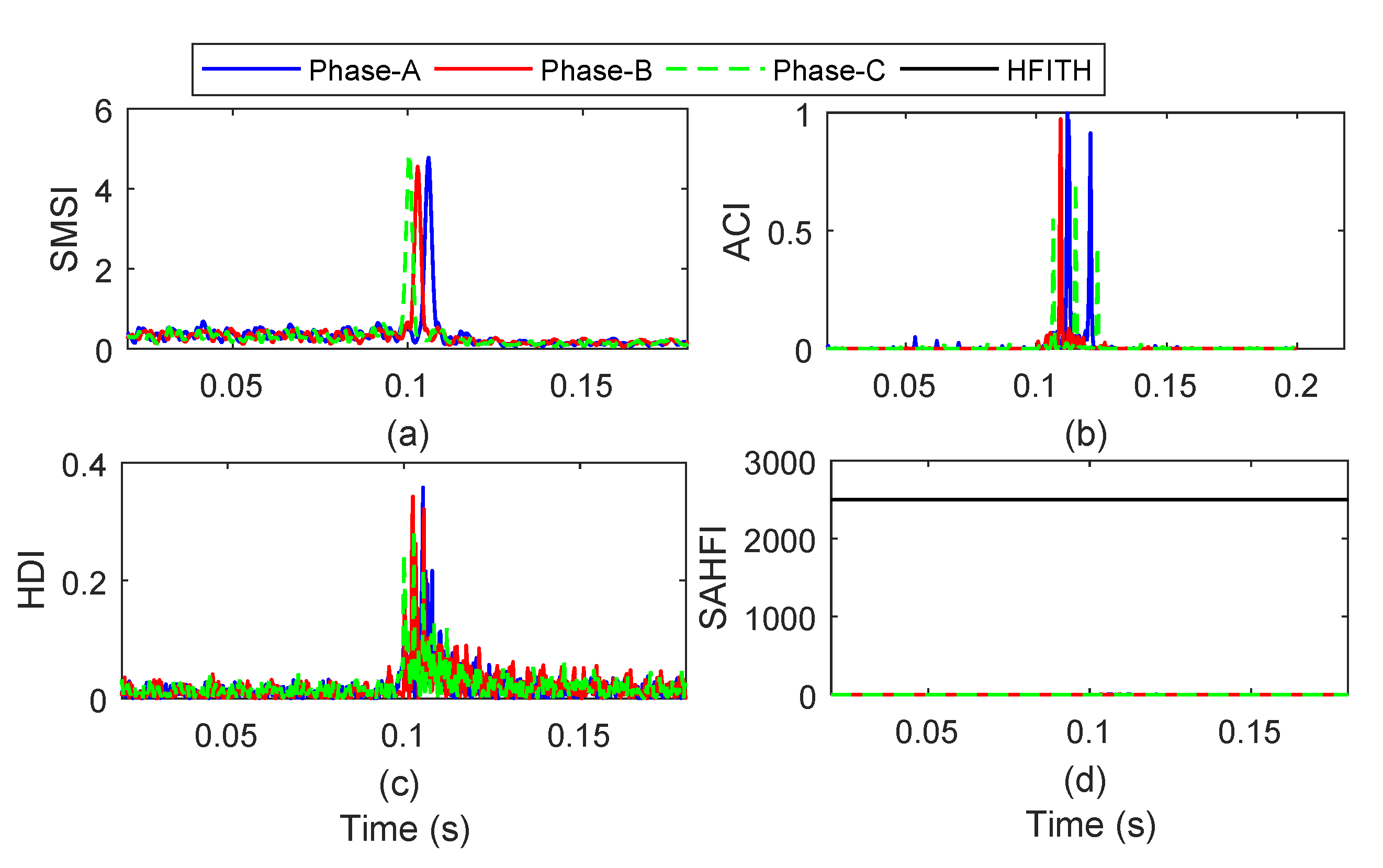
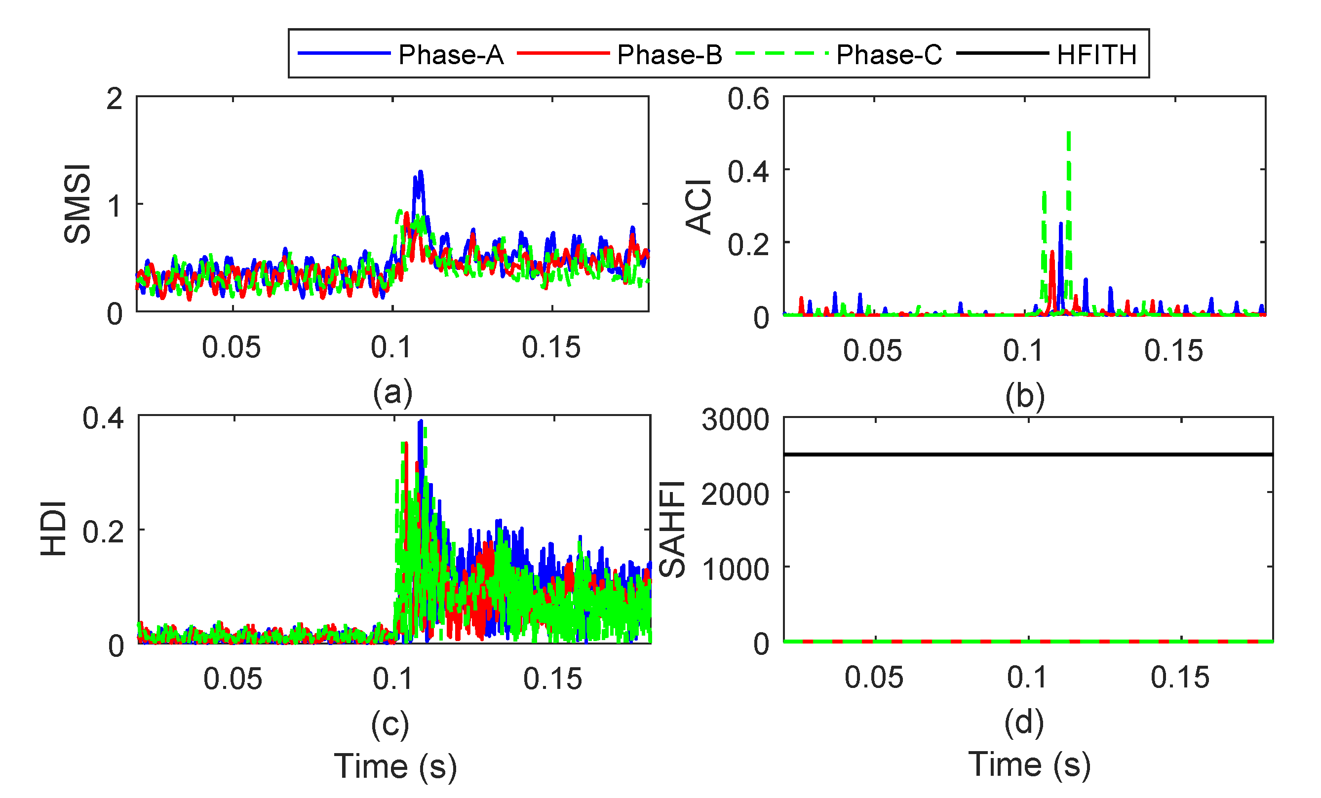
3.1. Stockwell Transform-Based Median and Summation Index

The current signals are recorded on the bus 650, which is designated as the hybrid grid protection relay location node (HGPRLN). These current signals are processed using the Stockwell Transform (ST) to propose a Stockwell Transform based Median and Summation Index (SMSI) for recognition of fault conditions on the grid. The ST can be evaluated either by the use of the continuous WT (CWT) or the short time Fourier transform (STFT). The ST is effective for extraction of the information hidden in the phase spectrum and amplitude of the current signal. This information is obtained in the form of a complex matrix designated as STM. Each row of this matrix indicates definite frequency and each column indicates the definite time. High time resolution at a high frequency and a low time resolution at a low frequency is achieved using the ST. This has the additional advantage that there is minimum effect of noise on its performance and effectively identify the distortions of the waveform [28]. The current signal ($i\left(t\right)$) is decomposed using the short time Fourier transform (STFT), and output (STI) is computed as described below [29].

$$STI(\tau ,f)={\int }_{-\infty }^{+\infty }i\left(t\right)g(\tau -t)e^{-j2\pi ft}dt,$$

(1)

where t and f are, respectively, the spectral localization time and Fourier frequency, and $g\left(t\right)$ represents the window function. The following Gaussian function ($g\left(t\right)$) is used in the above equation to evaluate the Stockwell Transform-based decomposition of $i\left(t\right)$ [30].

$$g\left(t\right)=\frac{\left|f\right|}{\sqrt{2\pi }}{e}^{-\frac{f^2{t}^2}{2}}.$$

(2)

Hence, the output matrix (which is complex in nature) of the Stockwell Transform-based decomposition of current signals (STM) can be given by the following relation [31].

$$STM(\tau ,f)={\int }_{-\infty }^{+\infty }i\left(t\right)\frac{\left|f\right|}{\sqrt{2\pi }}{e}^{-\frac{f^2{(\tau -t)}^2}{2}}{e}^{-j2\pi ft}dt.$$

(3)

This complex values STM matrix is used to extract the information of frequency and amplitude of the current signals. First, this complex values matrix is converted in a matrix with absolute values (AVM) using the following command.

$$AVM=abs\left(STM\right).$$

(4)

Median of the matrix AVM is evaluated using the below detailed command.

$$MV=median\left(AVM\right).$$

(5)

The summation of each column of the AVM is evaluated using the below detailed command.

$$SV=sum\left(AVM\right).$$

(6)

The MV and SV are multiplied element by element to compute the Stockwell Transform based median and summation index (SMSI) using the below detailed command.

$$SMSI=MV\times SV.$$

(7)

3.2. Hilbert Transform-Based Derivative Index

Hilbert Transform (HT) is a signal processing approach, which can be implemented for the purpose of protection schemes. This is effective for spectral analysis and provide description of time-frequency-energy of the voltage time series data. The HT is effective for computation of the momentary frequencies, as well as amplitudes, which can be used for description of the voltage signals. Hence, HT can be effectively used for recognition of the fault conditions in the hybrid grid with RE penetration. The HT supported decomposition of voltage signals can be computed using the below mentioned relation [32].

$$HT(v\left(t\right))=\frac{1}{\pi }PV{\int }_{-\infty }^{+\infty }\frac{v\left(\tau \right)}{t-\tau }d\tau .$$

(8)

Here, $PV$: Cauchy’s principle value integral, t: time, and $\tau$: time period. The voltage signal is used to compute Hilbert Transform-based derivative index (HDI). Voltage signal $v\left(t\right)$ is decomposed using the Hilbert Transform to evaluate output matrix with absolute values (HTI) using the following command.

$$HTI=abs\left(hilbert\right(v\left(t\right)\left)\right).$$

(9)

The HTI is differentiated with respect to time for computing the HDI as detailed below.

$$HDI=\frac{d\left(HTI\right)}{dt}.$$

(10)

This method has the merit that it gives physical instantaneous frequencies for voltage signal and minimum time for identification of the fault condition.

3.3. Alienation Coefficient Index

The sample supported alienation coefficient of voltage signals is computed for recognition of the faults and assigned the name Alienation Coefficient index (ACI). The correlation coefficient (CRC) between two voltage variables $v_1$ and $v_2$ is computed using the following relation [18].

$$r={\displaystyle \frac{N_s\sum v_1{v}_2-(\sum v_1)(\sum v_2)}{\sqrt{[N_s\sum v_1^2-{(\sum v_1)}^2][N_s\sum v_2^2-{(\sum v_2)}^2]}}}.$$

(11)

Here, symbol representation, Ns: sample numbers in a cycle (Ns = 32 with sampling frequency of $1.92$ kHz), $v_1$: samples of voltage at time $t_0$, $v_2$: samples of voltage at time $-T+t_0$, and T: time period. The ACI is computed using CRC by the following relation.

$$ACI=1-CR{C}^2.$$

(12)

The moving window approach is used to compute ACI for a period of the quarter cycle. Here, samples of the quarter cycle considered are compared with the samples of the corresponding quarter cycle of past cycle, and the window is moved in forward direction with one sample step every time. This process is repeated. ACI helps to reduce the time of fault recognition due to the feature of sharp change at fault incidence moment, resulting in the fast protection scheme.

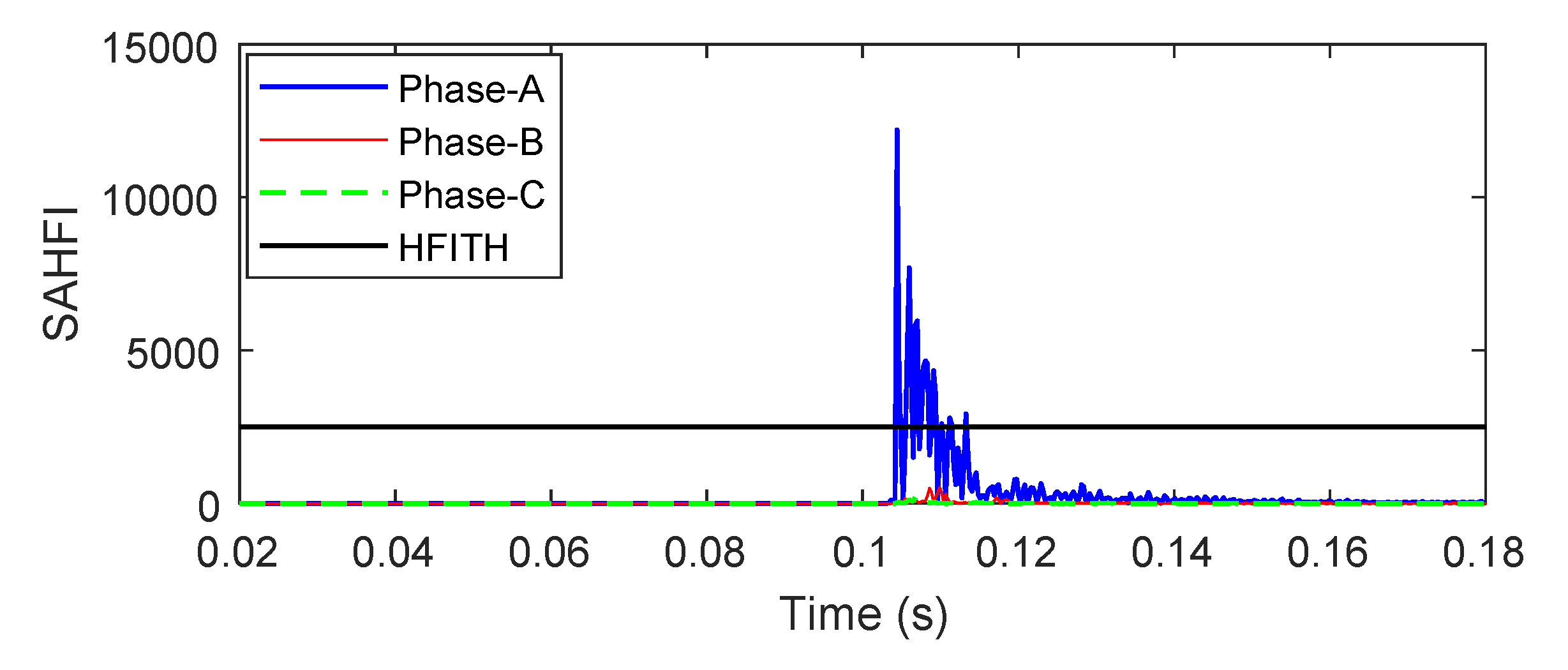
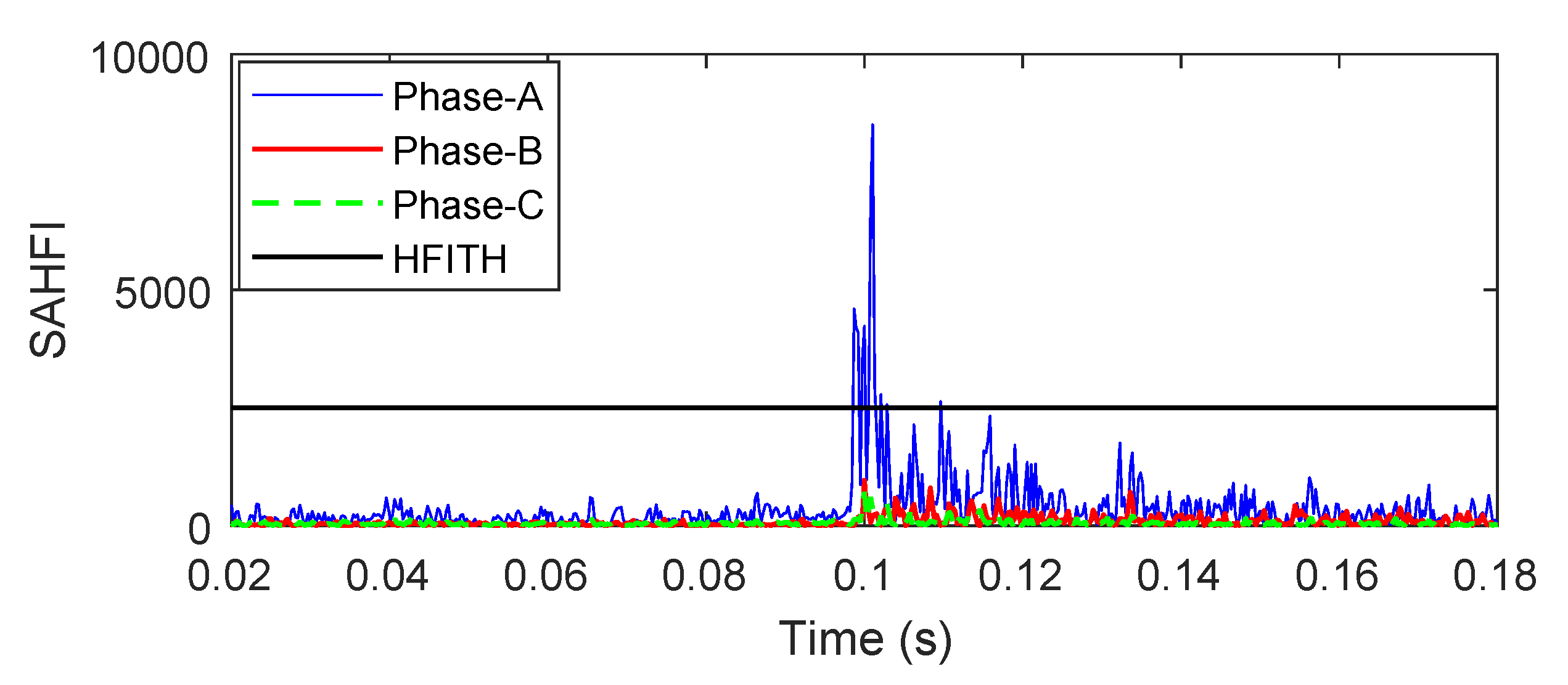
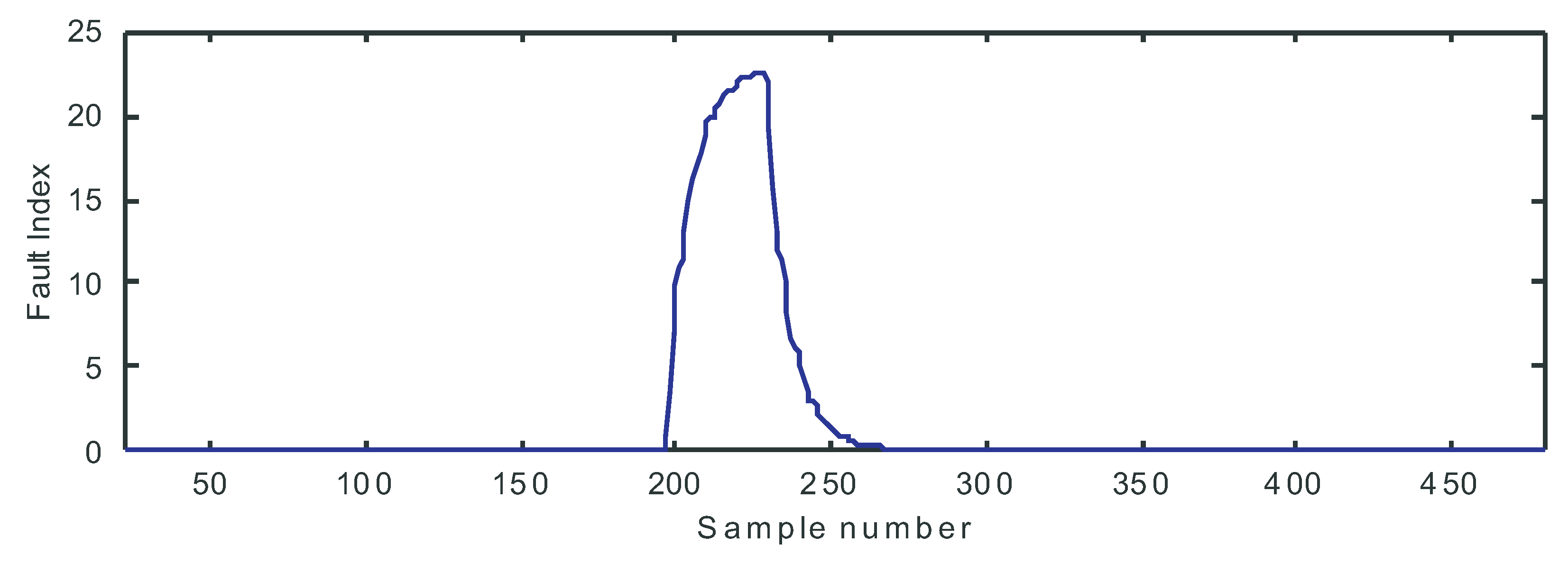
3.4. Stockwell, Alienation, and Hilbert Fault Index

The SMSI, HDI, and ACI are used to compute the Stockwell-, Hilbert-, and Alienation-based fault index (SAHFI), which is used to identify the different fault conditions. The SAHFI is evaluated using the multiplication of the SMSI, ACI, and HDI as detailed below.

$$SAHFI=SMSI\times ACI\times HDI\times W.$$

(13)

Here, W: weight factor, which is taken as 100. This WF may be set depending on the complexity of the network and penetration level of the renewable energy at the time of installation of protection scheme. A threshold value of 2500 is selected for the SAHFI and designated as hybrid fault index threshold (HFITH). This algorithm has the merits that its performance is least affected by noise, recognizes fault conditions in minimum time, reduces the time of fault recognition, effectively recognizes the fault conditions in different scenarios of the grid, and is free from generation of false tripping command.

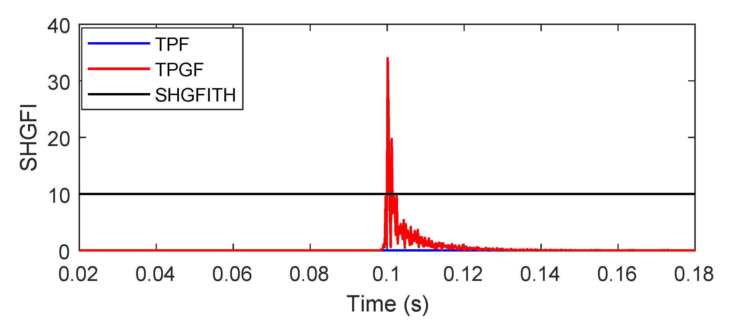
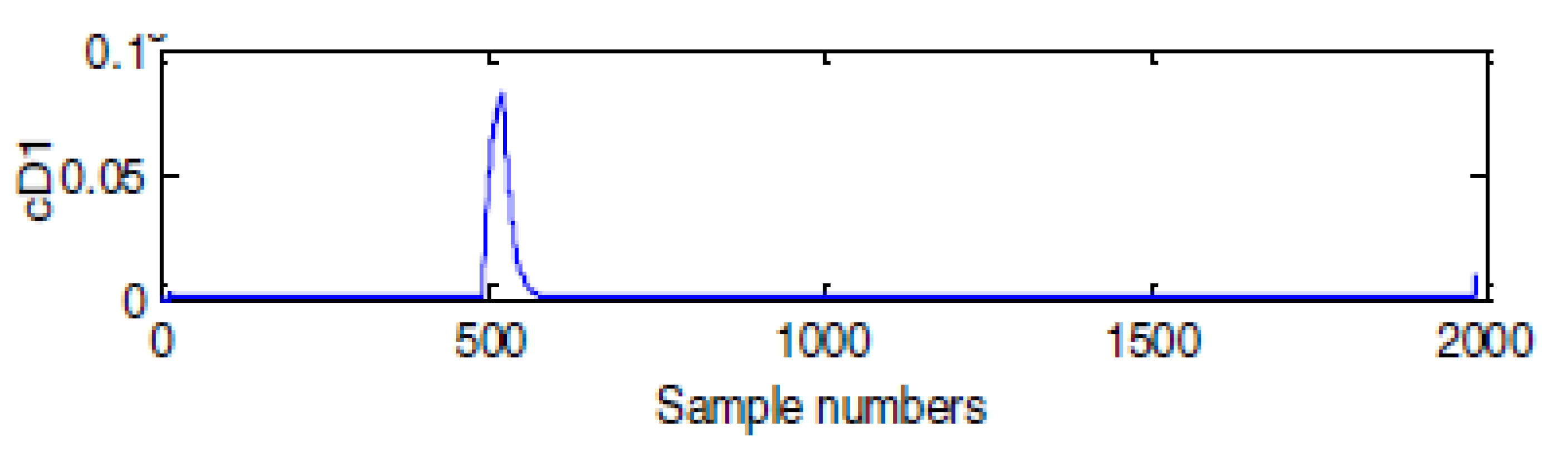
3.5. Stockwell Transform- and Hilbert Transform-Based Ground Fault Index

A Stockwell Transform and Hilbert Transform based ground fault index (SHGFI) is introduced to categorize the phase and ground (PGF) fault and any two phases (TPF) fault. This is also used to categorize all three phases and ground (ATPGF) fault and all three phases (ATPF) fault. Following procedure is used to find the SHGFI:-

• Calculate the zero sequence current ($I_0$) using the currents $I_1$, $I_2$, and $I_3$ associated with phases A, B, and C, respectively, using the following relation.

  $$I_0=\frac{I_1+I_2+I_3}{3}.$$

  (14)
• Calculate the $SMS{I}_0$ using the mathematical formulation detailed in Section 3.1 by processing the zero sequence current.
• Calculate the $HD{I}_0$ using the mathematical formulation detailed in Section 3.2 by processing the zero sequence current.
• Calculate the SHGFI by multiplying the $SMS{I}_0$ and $HD{I}_0$ as detailed below:-

  $$SHGFI=SMS{I}_0\times HD{I}_0\times W_0.$$

  (15)
  Here, $W_0$ is weight factor for the SHGFI, which is considered as ${10}^3$ in this study. The threshold for the SHGFI (SHGFITH) is taken as 10 to detect the involvement of ground during the faulty condition.

4. Recognition of Fault Conditions: Results of Simulation

Results for implementation of the algorithm to identify and classify the fault conditions for protection of the grid network in the presence of RE are discussed in this section. The fault conditions, which include a phase and ground (PGF), any two phases (TPF), any two phases and ground (TPGF), all three phases (ATPF), and all three phases and ground (ATPGF), are analyzed. Results to classify the fault conditions are also discussed. The test bus 675 is considered as fault condition node (FCN) and voltage and currents are measured on test bus 650, which is considered as hybrid grid protection relay location node (HGPRLN).

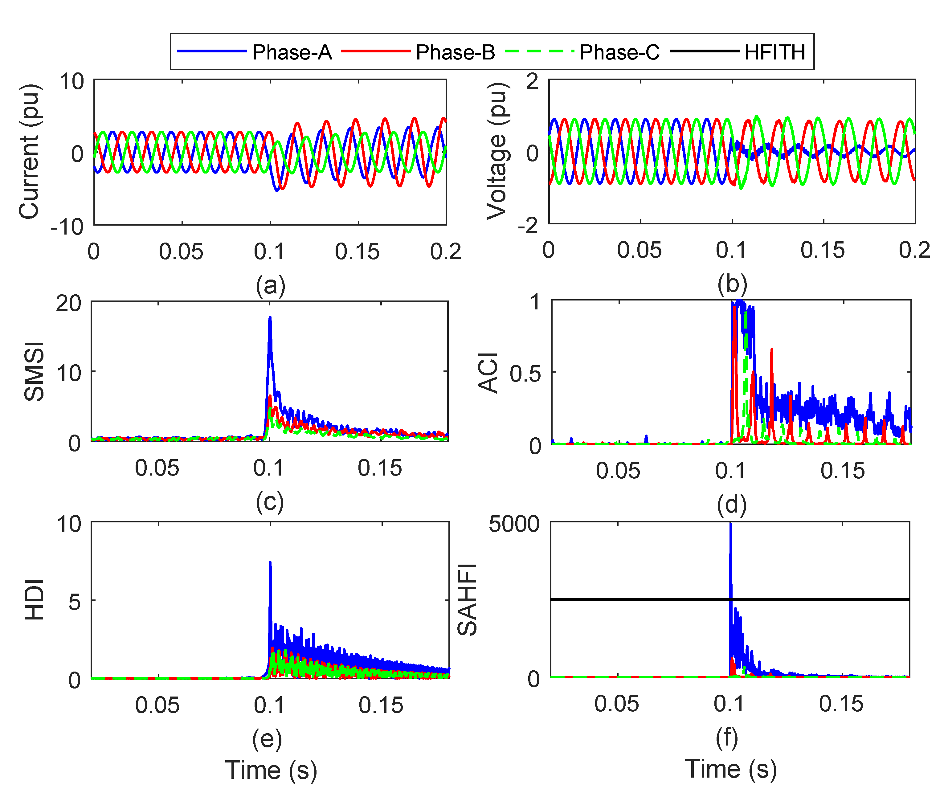
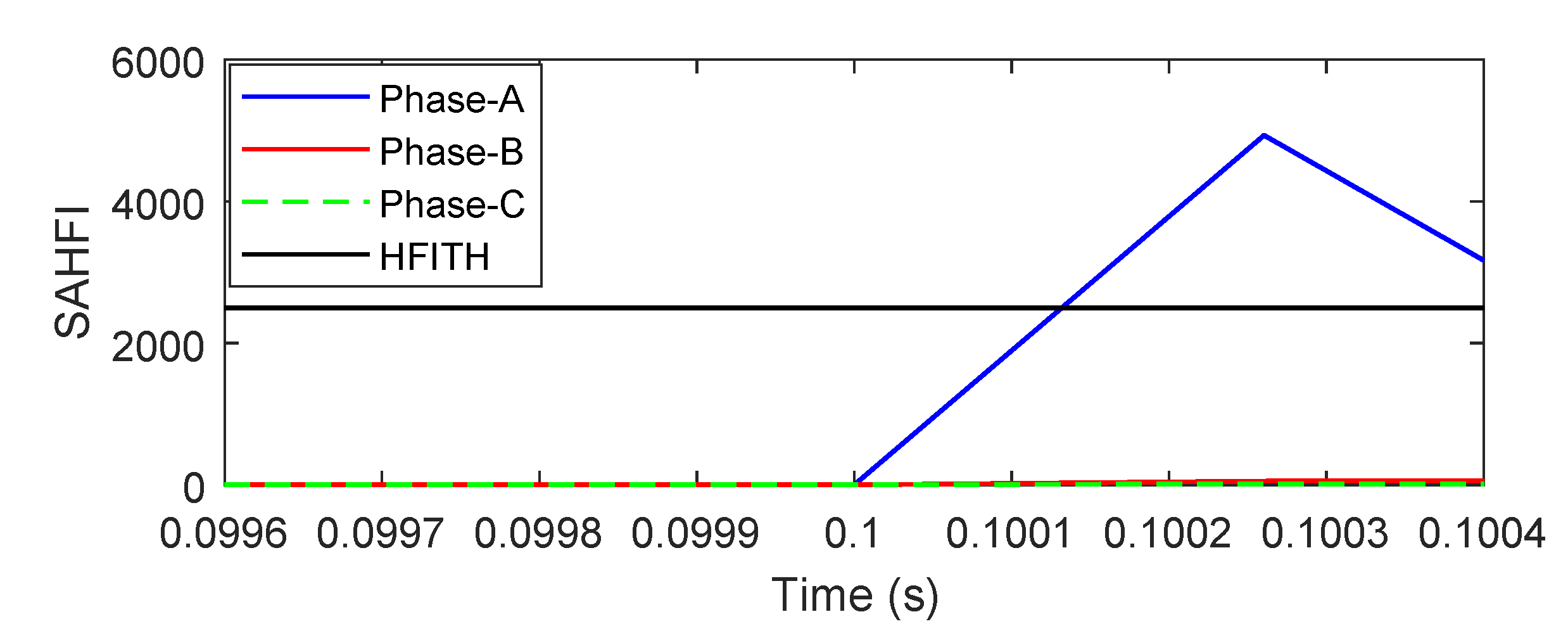
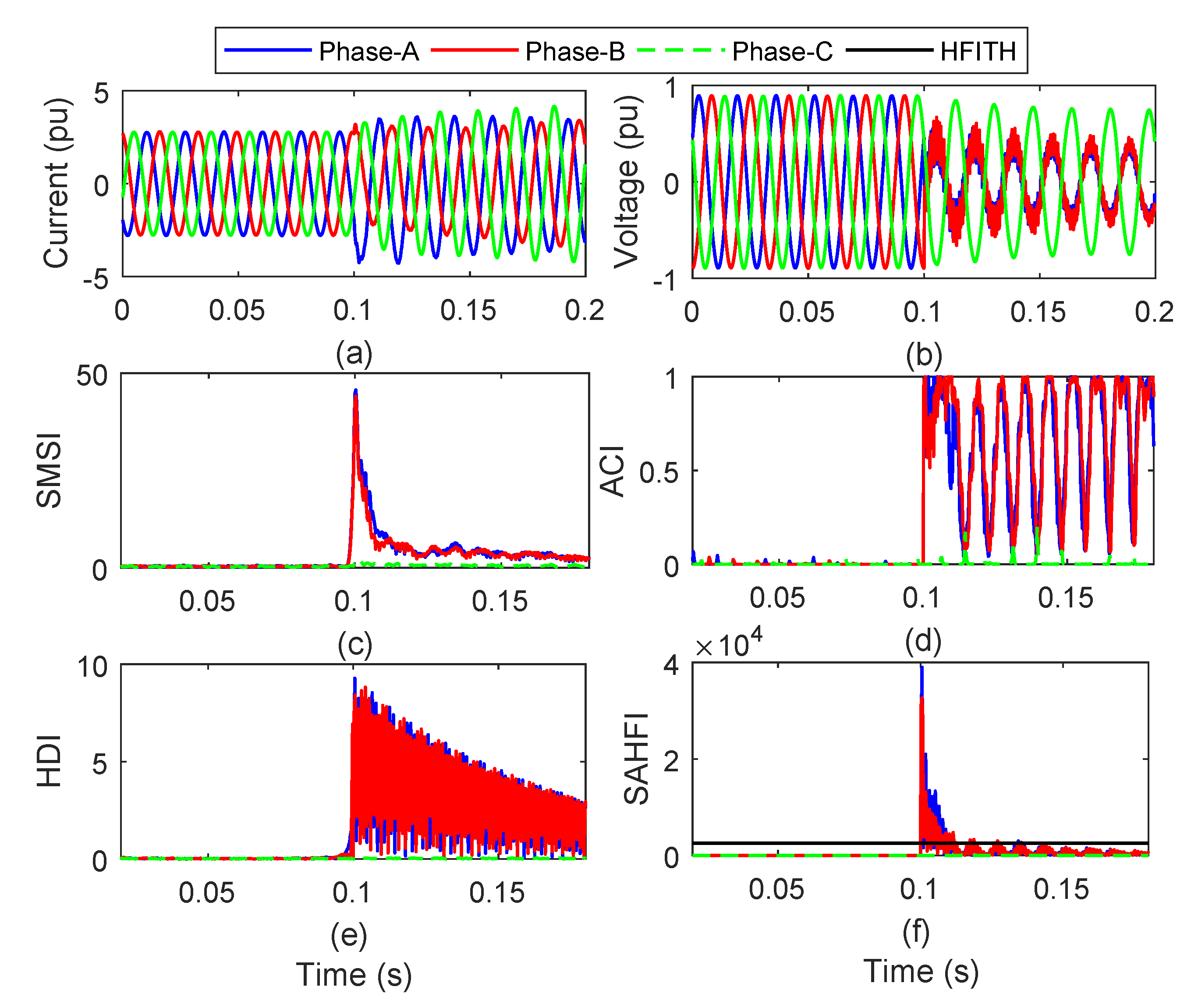
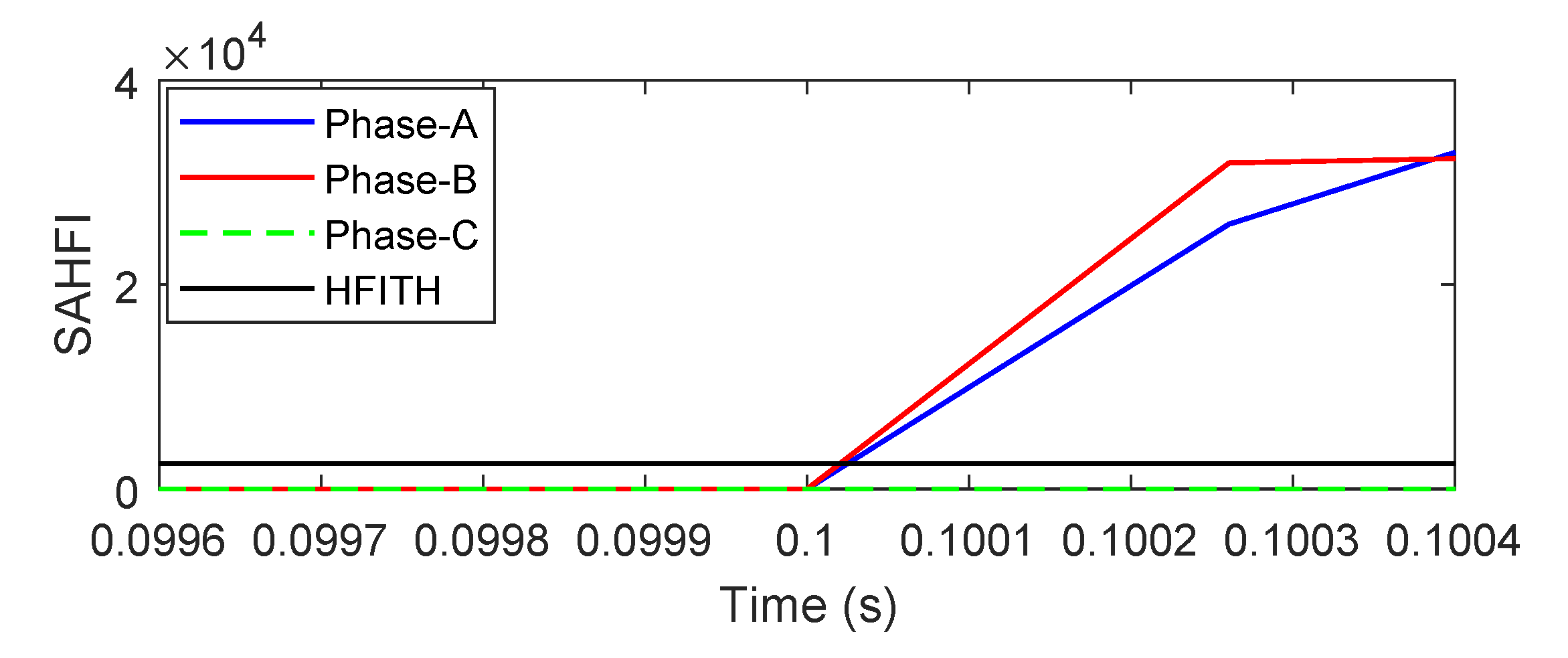
4.1. Fault Condition Involving Ground and Phase A

A fault condition involving ground and phase A (PGF) is executed at $0.1$ s on FCN of the grid with RE sources. Signals of voltage and current are recorded at the HGPRLN. The current signals are processed using the ST to compute the SMSI. The voltage signals are processed using the Hilbert Transform to compute the HDI. The voltage signals are also processed using the Alienation Coefficient to compute the ACI. The SAHFI for PGF condition is computed using the SMSI, ACI, and HDI. The current signals, voltage signals, SMSI, ACI, HDI, and SAHFI for a PGF on phase A are described in Figure 3 in respective order. Figure 3c details that, due to the incidence of PGF on phase A, increase in the SMSI for phase A is high compared to the SMSI of phases B and C. This index has low values during the healthy condition. Figure 3d details that, due to the incidence of PGF on phase A, the ACI increases corresponding to all phases. This index also has low values during the healthy condition and increases sharply due to incidence of fault condition. Figure 3e details that, due to the incidence of PGF on phase A, increase in the HDI for phase A is high compared to the HDI of phases B and C. This index also has low values during the healthy condition. Figure 3f details that, due to the incidence of PGF on phase A, the proposed SAHFI has peak magnitude above the HFITH (2500) for phase A, whereas this index for phases B and C is below the HFITH. Hence, the condition of the PGF on phase A is effectively recognized using the proposed algorithm. This algorithm is also effective to recognize the PGF fault condition on phases B and C.

A high resolution version of the SAHFI at the moment of incidence of PGF condition (phase A) is shown in Figure 4. The SAHFI associated with the faulty phase A achieves the value equal to HFITH (2500) at $0.10015$ s after a time interval of $0.15$ ms after fault incidence. Hence, the PGF event is detected in a time duration of $(1/110)$th fraction of a time of one cycle.

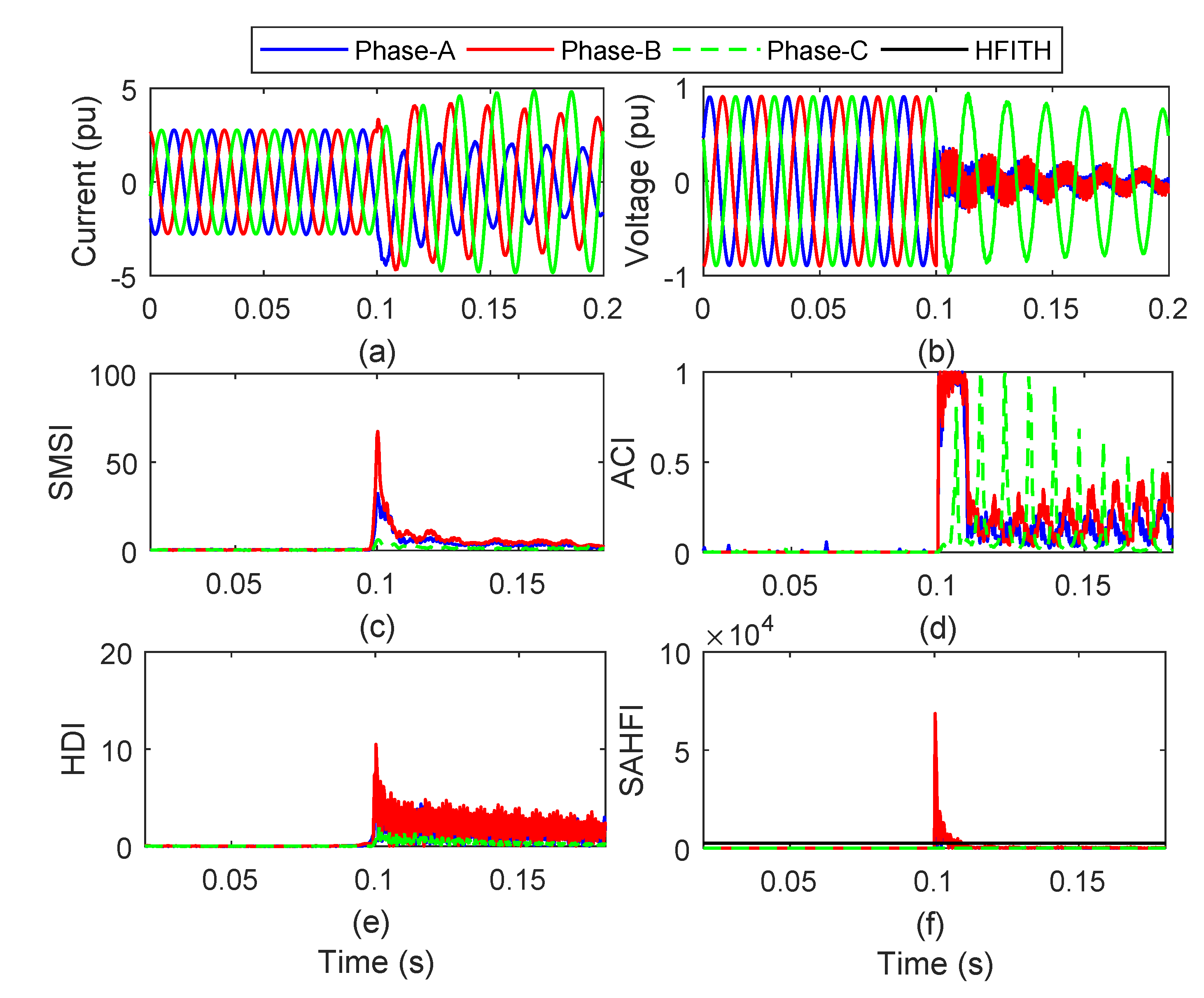
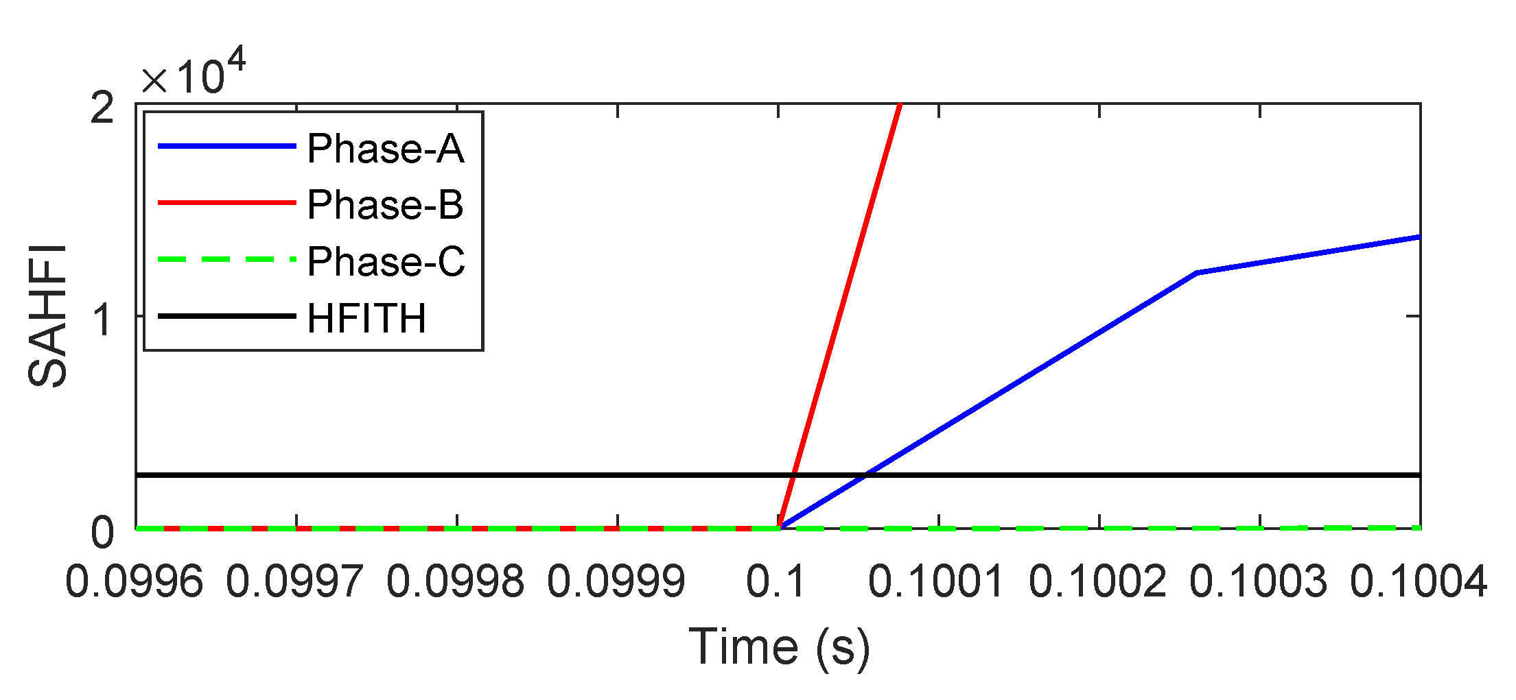
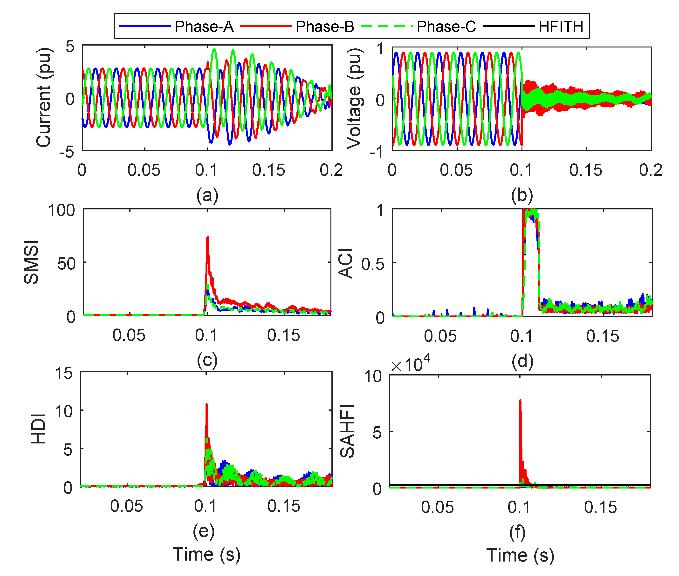
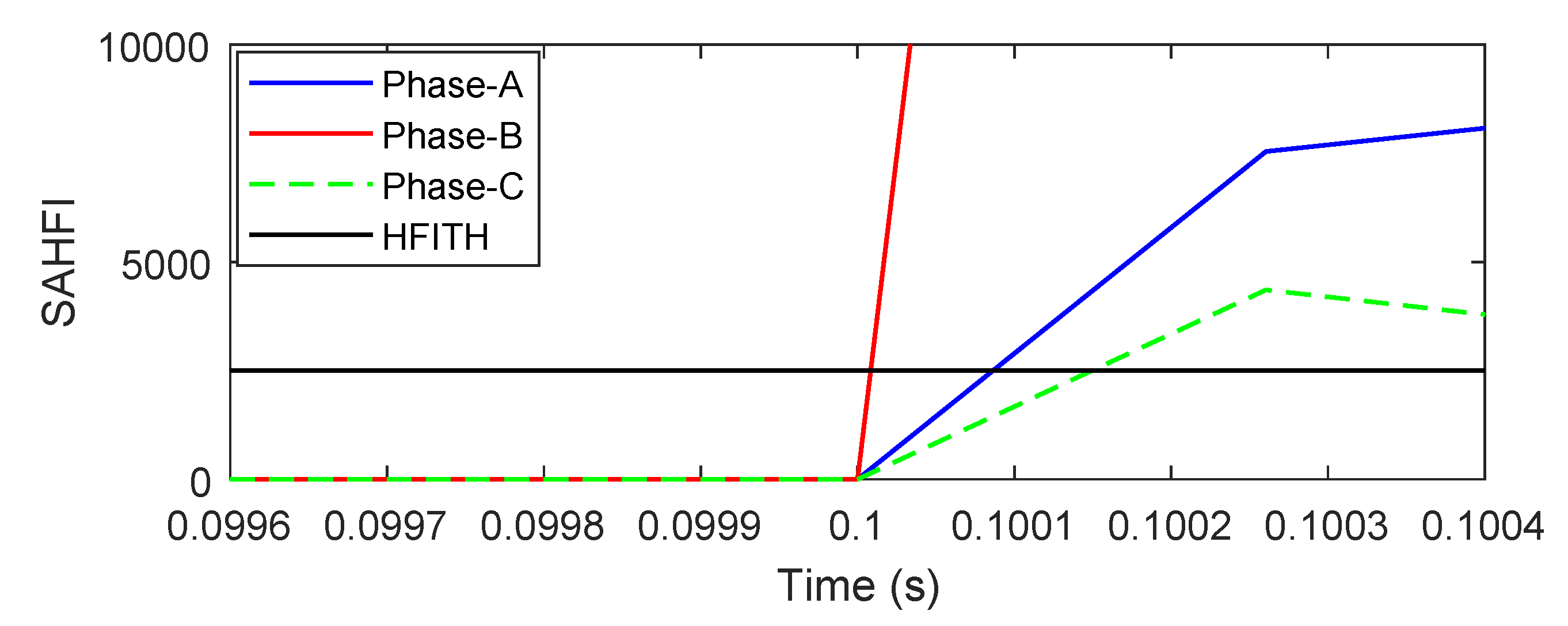
4.2. Fault Condition Involving Two Phases

A two phases fault (TPF) condition involving phases A and B is executed at $0.1$ s on FCN of the grid with RE sources. Signals of voltage and current are recorded at the HGPRLN. The current signals are processed using the ST to compute the SMSI. The voltage signals are processed using the Hilbert Transform to compute the HDI. The voltage signals are also processed using the Alienation Coefficient to compute the ACI. The SAHFI for TPF condition is computed using the SMSI, ACI, and HDI. The current signals, voltage signals, SMSI, ACI, HDI, and SAHFI for a TPF condition involving phases A and B are described in Figure 5 in respective order. Figure 5c details that, due to the incidence of the TPF on phases A and B, increase in the SMSI for phases A and B is high, and this SMSI is low for phase C. This index has low values during the healthy condition. Figure 5d details that, due to the incidence of TPF condition on phases A and B, the ACI increases corresponding to all phases. This index also has low values during the healthy condition and increase sharply due to incidence of TPF fault condition. Figure 5e details that, due to the incidence of TPF on phases A and B, increase in the HDI for phases A and B is high compared to the HDI of phase C. This index also has low values during the healthy condition. Figure 5f details that, due to the incidence of TPF on phases A and B, the proposed SAHFI has peak magnitude above the HFITH (2500) for phases A and B, whereas this index for phase C is below the HFITH. Hence, the condition of the TPF on phases A and B is effectively recognized using the proposed algorithm. This algorithm is also effective to recognize the TPF fault condition involving other combinations of phases, such as B and C and C and A.

A high resolution version of the SAHFI at the moment of incidence of TPF condition on phases A and B is shown in Figure 6. The SAHFIs associated with the faulty phases A and B achieve the value equal to HFITH (2500) at $0.10002$ s in a time interval of $0.02$ ms after fault incidence. Hence, the PGF event is detected in a time duration of $(1/830)$th fraction of a time period of one cycle.

4.3. Fault Condition Involving Two Phases and Ground

A two phases fault condition involving phases A and B and ground (TPGF) is executed at $0.1$ s on FCN of the grid with RE sources. Signals of voltage and current are recorded at the HGPRLN. The current signals are processed using the ST to compute the SMSI. The voltage signals are processed using the Hilbert Transform to compute the HDI. The voltage signals are also processed using the Alienation Coefficient to compute the ACI. The SAHFI for TPF condition is computed using the SMSI, ACI, and HDI. The current signals, voltage signals, SMSI, ACI, HDI, and SAHFI for a TPGF condition involving phases A and B are described in Figure 7 in respective order. Figure 7c details that, due to the incidence of TPGF on phases A and B, increase in the SMSI for phases A and B is high and this SMSI is low for phase C. This index has low values during the healthy condition. Figure 7d details that, due to the incidence of TPGF condition on phases A and B, the ACI increases corresponding to all phases. This index also has low values during the healthy condition and increase sharply due to incidence of TPGF fault condition. Figure 7e details that, due to the incidence of TPGF on phases A and B, increase in the HDI for phases A and B is high compared to the HDI of phase C. This index also has low values during the healthy condition. Figure 7f details that, due to the incidence of TPGF on phases A and B, the proposed SAHFI has peak magnitude above the HFITH (2500) for phases A and B, whereas this index for phase C is below the HFITH. Hence, the condition of the TPGF on phases A and B is effectively recognized using the proposed algorithm. This algorithm is also effective to recognize the TPGF fault condition involving other combinations of phases, such as B and C and C and A.

A high resolution version of the SAHFI at the moment of incidence of TPGF condition on phases A and B is shown in Figure 8. The SAHFI associated with the faulty phase A achieves the value equal to HFITH (2500) at $0.10005$ s after a time interval of 0.5 ms after fault incidence. This SAHFI associated with the faulty phase B achieves the value equal to HFITH (2500) at $0.10001$ s after a time interval of $0.1$ ms after fault incidence. Hence, the TPGF event is detected in a time duration of $(1/330)$th fraction of a time duration of one cycle.

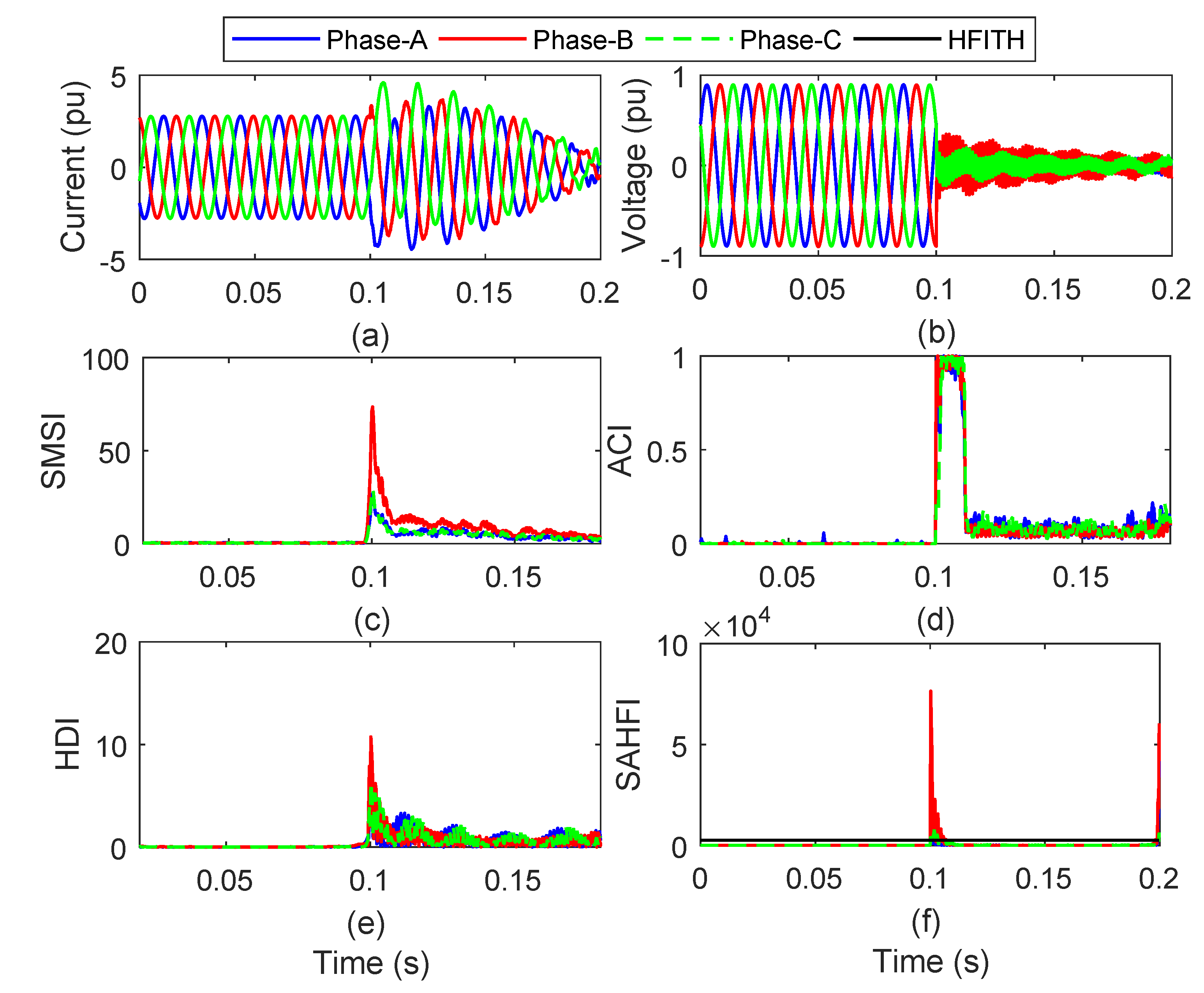
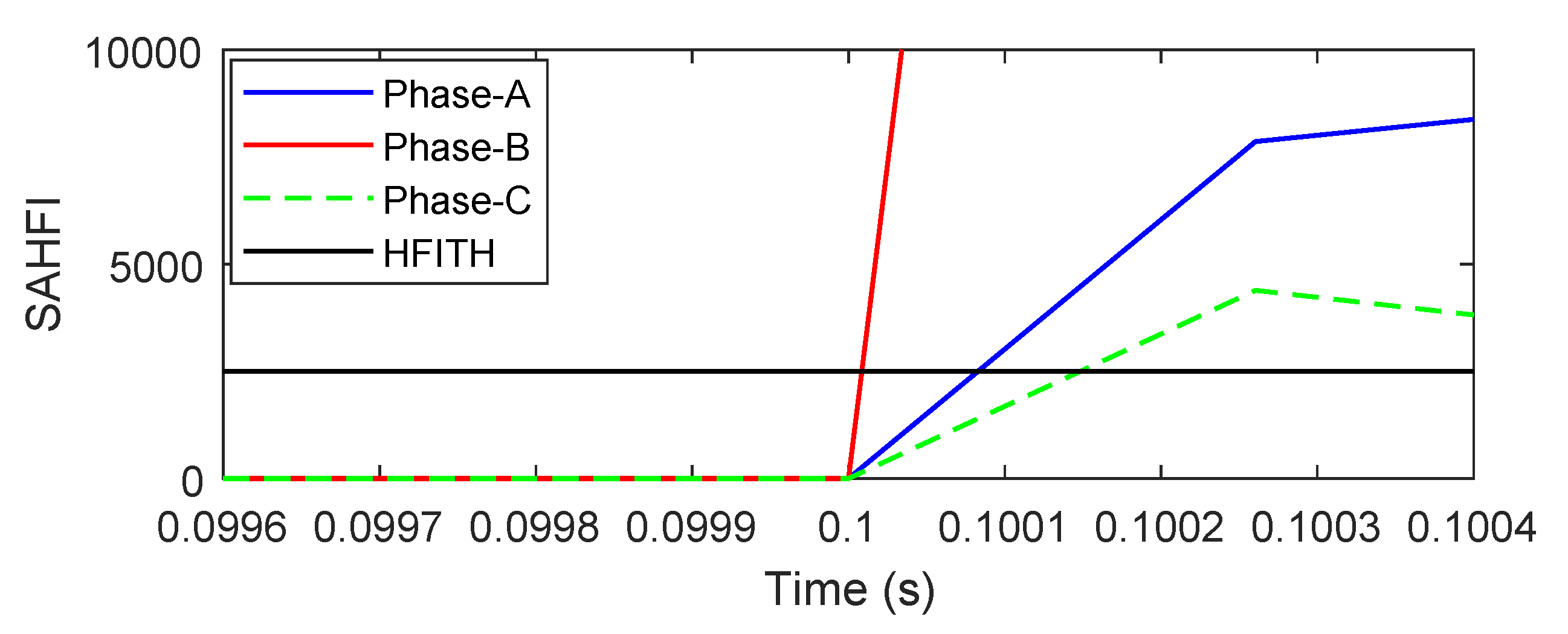
4.4. Fault Involving All the Phases

An all the three phases fault (ATPF) condition involving all phases is executed at $0.1$ s on FCN of the grid with RE sources. Signals of voltage and current are recorded at the HGPRLN. The current signals are processed using the ST to compute the SMSI. The voltage signals are processed using the Hilbert Transform to compute the HDI. The voltage signals are also processed using the Alienation Coefficient to compute the ACI. The SAHFI for ATPF condition is computed using the SMSI, ACI, and HDI. The current signals, voltage signals, SMSI, ACI, HDI, and SAHFI for a TPF condition involving all the phases are described in Figure 9 in respective order. Figure 9c details that, due to the incidence of ATPF on all phases, increase in the SMSI for all phases is high. This index has low values during the healthy condition. Figure 9d details that, due to the incidence of ATPF condition on all phases, the ACI increases corresponding to all phases. This index also has low values during the healthy condition and increase sharply due to incidence of ATPF fault condition. Figure 9e details that, due to the incidence of ATPF on all phases, increase in the HDI for all phases is high. This index also has low values during the healthy condition. Figure 9f details that, due to the incidence of ATPF on all phases, the proposed ATPF has peak magnitude above the HFITH (2500) for all the phases. Hence, the condition of the ATPF on all the phases is effectively recognized using the proposed algorithm.

A high resolution version of the SAHFI at the moment of incidence of ATPF condition on all the phases is shown in Figure 10. The SAHFI associated with phase A achieves the value equal to HFITH (2500) at $0.10008$ s after a time interval of $0.08$ ms after fault incidence. This SAHFI associated with the faulty phase B achieves the value equal to HFITH (2500) at $0.10001$ s after a time interval of $0.001$ ms after fault incidence. Similarly, this SAHFI associated with the faulty phase C achieves the value equal to HFITH (2500) at $0.10015$ s after a time interval of $0.15$ ms after fault incidence. Hence, the ATPF event is detected in a time duration of $(1/110)$th fraction of a time duration of one cycle.

4.5. Fault Involving All the Phases and Ground

An all the three phases to ground fault (ATPGF) condition involving all phases is executed at $0.1$ s on FCN of the grid with RE sources. Signals of voltage and current are recorded at the HGPRLN. The current signals are processed using the ST to compute the SMSI. The voltage signals are processed using the Hilbert Transform to compute the HDI. The voltage signals are also processed using the Alienation Coefficient to compute the ACI. The SAHFI for ATPGF condition is computed using the SMSI, ACI, and HDI. The current signals, voltage signals, SMSI, ACI, HDI, and SAHFI for an ATPGF condition are described in Figure 11 in respective order. Figure 11c details that, due to the incidence of ATPGF on all the phases, increase in the SMSI for all phases is high. This index has low values during the healthy condition. Figure 11d details that, due to the incidence of ATPGF condition on all the phases, the ACI increases corresponding to all the phases. This index also has low values during the healthy condition and increase sharply due to incidence of ATPGF fault condition. Figure 11e details that, due to the incidence of ATPGF on all the phases, increase in the HDI for all phases is high. This index also has low values during the healthy condition. Figure 11f details that, due to the incidence of ATPGF on all the phases, the proposed ATPGF has peak magnitude above the HFITH (2500) for all the phases. Hence, the condition of the ATPGF on all the phases is effectively recognized using the proposed algorithm.

A high resolution version of the SAHFI at the moment of incidence of ATPGF condition on all the phases is shown in Figure 12. The SAHFI associated with phase A achieves the value equal to HFITH (2500) at $0.10008$ s after a time interval of $0.08$ ms after fault incidence. This SAHFI associated with the faulty phase B achieves the value equal to HFITH (2500) at $0.10001$ s after a time interval of $0.001$ ms after fault incidence. Similarly, this SAHFI associated with the faulty phase C achieves the value equal to HFITH (2500) at $0.10015$ s after a time interval of $0.15$ ms after fault incidence. Hence, an ATPGF event is detected in a time duration of $(1/110)$th fraction of a time interval of one cycle.

5. Categorization of Fault Conditions

The fault conditions are categorized using the number of phases involved in the fault. The phases involved in the fault condition are recognized using the proposed SAHFI for a phase and comparing with the HFITH (2500). A faulty phase has a peak value of SAHFI higher compared to the HFITH, whereas this index has a peak value below HFITH for healthy phases. If only one phase is faulty then PGF fault is present. Two phases will be faulty during the conditions of TPF or the TPGF faults. All the three phases will be faulty when either the ATPF or the ATPGF fault is present.

There are two faulty phases during the events of TPF and TPGF. A Hilbert Transform and Stockwell Transform-based ground fault index (SHGFI) is introduced to categorize the TPF and TPGF faults, which is detailed in Figure 13. This is observed that for the event of TPF, the SHGFI has low values near to zero, whereas this index has a high magnitude peak for the TPGF faulty event at the time of fault incidence, which crosses the threshold value of SHGFI (SHGFITH). Here, SHGFITH is considered equal to 10. Therefore, it is concluded that the proposed method is effective in the categorization of all the types of investigated fault conditions. Similarly, the ATPF and ATPGF fault events are also successfully identified using the SHGFI.

6. Case Studies: Implementation of Protection Algorithm

The protection approach is validated for different fault conditions, such as different values of impedance during fault condition, fault incident angle (FIA), different FCN, and noisy condition. Results for the PGF condition are elaborated in this section. However, the protection approach is equally effective for the conditions of TPF, TPGF, ATPF, and ATPGF.

6.1. Impact of Fault Impedance

The algorithm is tested for different values of the impedance involved during the fault condition. The algorithm is tested for fault impedance values of $0\Omega$, $2\Omega$, $4\Omega$, $6\Omega$, $8\Omega$, and $10\Omega$ during the PGF fault condition and peak magnitudes of respective SAHFI are tabulated in

Table 2. Peak magnitude of SAHFI for PGF condition with different fault impedance.

Phase	Peak of SAHFI
	$\mathbf{0}\mathbf{\Omega }$	$\mathbf{2}\mathbf{\Omega }$	$\mathbf{4}\mathbf{\Omega }$	$\mathbf{6}\mathbf{\Omega }$	$\mathbf{8}\mathbf{\Omega }$	$\mathbf{10}\mathbf{\Omega }$
A	4933	4704	4511	4398	4082	3804
B	$600.2$	$583.5$	$598.6$	$533.9$	$508.4$	$498.7$
C	$359.2$	$341.7$	$328.2$	$313.5$	$297.1$	$278.1$

. From this it is inferred that SAHFI has a peak magnitude higher than the HFITH (2500) for phase A and lower for phases B and C for all the values of investigated fault impedances. Therefore, the PGF fault event is effectively recognized for the fault impedance values up to $10\Omega$. The algorithm is also effective in recognizing the TPF, TPGF, ATPF, and ATPGF fault conditions for the fault impedance values up to $10\Omega$.

6.2. Impact of FCN

Location of the fault at different buses of the test grid affects the SAHFI. Hence, the algorithm is tested by realizing the fault at different nodes. The peak magnitude of SAHFI during the condition of PGF at various nodes of the test grid in the presence of RE generation are tabulated in

Table 3. Peak magnitude of SAHFI for PGF condition at different FCN.

FCN	Peak of SAHFI
	Phase A	Phase B	Phase C
675	4933	$600.2$	$359.2$
611	5024	$604.1$	$362.7$
652	4526	$587.6$	$342.9$
680	$7.263\times {10}^4$	$805.1$	$545.01$
634	4229	$559.4$	$329.8$
646	8116	$682.3$	$401.5$

. From this it is inferred that SAHFI has peak magnitude higher than the HFITH (2500) for phase A and lower for phases B and C for all the locations of the faults. Therefore, the PGF fault event is effectively recognized when there is a fault incident at various nodes of the test grid. The algorithm is also effective in recognizing the TPF, TPGF, ATPF, and ATPGF fault conditions at different nodes.

6.3. Impact of Fault Incidence Angle

A fault condition of PGF on phase A is executed at 0.01 s with fault incident angle (FIA) of 90° of the waveform on FCN of the grid with RE sources. Signals of voltage and current are recorded at the HGPRLN. The current signals with FIA of 90° are processed using ST to compute the SMSI. The voltage signals with FIA of 90° are processed using the Hilbert Transform to compute the HDI. The voltage signals with FIA of 90° are also processed using the Alienation Coefficient to compute the ACI. The SAHFI for the PGF condition is computed using the SMSI, ACI, and HDI, which is illustrated in Figure 14. Figure 14 details that, due to the incidence of PGF condition on phase A, the proposed SAHFI has a peak magnitude above the HFITH (2500) for phase A, whereas this index for phases B and C is below the HFITH. Hence, the condition of the PGF on phase A with FIA of 90° is effectively recognized using the proposed algorithm. It is also observed that the voltage magnitude of the SAHFI has increased significantly compared to the noise-free environment.

The peak magnitude of SAHFI during the condition of PGF with FIA of 0°, 45°, 90°, and 135° are tabulated in

Table 4. Peak magnitude of SAHFI for PGF condition with various FIAs.

Phase	Peak of SAHFI
	0°	45°	90°	135°
A	4933	$3.59\times {10}^4$	$1.22\times {10}^4$	4614
B	$600.2$	$857.8$	$716.1$	$548.5$
C	$359.2$	$725.2$	$691.2$	$304.2$

. From this it is inferred that SAHFI has peak magnitude higher than the HFITH (2500) for phase A and lower for phases B and C for all the FIAs. Therefore, the PGF fault event is effectively recognized for the different angles of incidence of faults.

6.4. Impact of Noise

A fault condition of PGF on phase A is executed at $0.1$ s on FCN of the grid with RE sources. Signals of voltage and current are recorded at the HGPRLN. A noise of level 20 dB SNR is superimposed on both the voltage and current signals. The current signals with noise of 20 dB SNR are processed using ST to compute the SMSI. The voltage signals with noise of 20 dB SNR are processed using the Hilbert Transform to compute the HDI. The voltage signals with noise of 20 dB Signal to noise ratio (SNR) are also processed using the Alienation Coefficient to compute the ACI. The SAHFI for PGF condition is computed using the SMSI, ACI, and HDI, which is illustrated in Figure 15. Figure 15 details that, due to the incidence of the condition on phase A, the proposed SAHFI has a peak magnitude above the HFITH (2500) for phase A, whereas this index for phases B and C is below the HFITH. Hence, the condition of the PGF on phase A with the superimposed noise of 20 dB SNR on both the voltage and current signals is effectively recognized using the proposed algorithm. It is also observed that the voltage magnitude of the SAHFI has increased significantly compared to the noise-free environment.

7. Performance of Protection Algorithm in the Presence of Switching Transients

It is expected that a protection scheme should not operate during the operational events, such as operation of a power plant, load, feeder, and capacitor banks. Hence, the section presents results for the operational conditions to establish that trip commands for the circuit breaker (CB) will not be generated during the operational events.

7.1. Tripping of Wind Plant

The wind power plant of capacity $1.5$ MW integrated on bus 680 is tripped at $0.01$ s. Signals of voltage and current are recorded at the HGPRLN. The current signals are processed using ST to compute the SMSI. The voltage signals are processed using the Hilbert Transform to compute the HDI. The voltage signals are also processed using the Alienation Coefficient to compute the ACI. The SAHFI for the event of wind plant tripping is computed using the SMSI, ACI, and HDI. The SMSI, ACI, HDI and SAHFI and described in Figure 16a–d in respective order. Figure 16a details that the magnitude of SMSI increase for all phases at instant of tripping of the wind plant. Figure 16b details that the magnitude of ACI increase for all phases at instant of tripping of the wind plant. Figure 16c details that the magnitude of HDI increase for all phases at instant of tripping of wind plant. Figure 16d details that the magnitude of the increase for all phases at instant of tripping of the wind plant, but the increase in the magnitude is much less compared to the SAHFITH (2500). Hence, the peak magnitude of the corresponding to all phases is below the SAHFITH. Therefore, a CB trip command will not be generated during this event of wind plant tripping, and the power system network will operate in normal operating condition.

7.2. Capacitor Bank and RL Load Operation

The load consisting of 843 kW and 462 kVAr and capacitor bank of 600 kVAr connected on bus 675 of the test system are simultaneously tripped at $0.1$ s. Signals of voltage and current are recorded at the HGPRLN. The current signals are processed using ST to compute the SMSI. The voltage signals are processed using the Hilbert Transform to compute the HDI. The voltage signals are also processed using the Alienation Coefficient to compute the ACI. The SAHFI for the PGF condition is computed using the SMSI, ACI, and HDI. The SMSI, ACI, HDI, and SAHFI for event of simultaneous tripping of capacitor bank and load are described in Figure 17a–d in respective order. Figure 17a details that magnitude of the SMSI increase for all phases at instant of simultaneous tripping of capacitor bank and load. Figure 17b details that the magnitude of the ACI increases for all phases at instant of simultaneous tripping of capacitor bank and load. Figure 17c details that the magnitude of the HDI increases for all phases at instant of simultaneous tripping of capacitor bank and load. Figure 17d details that the magnitude of the SAHFI increases for all phases at instant of simultaneous tripping of capacitor bank and load, but the the increase in magnitude is much less compared to the SAHFITH (2500). Hence, the peak magnitude of the SAHFI corresponding to all phases is below the SAHFITH. Therefore, a CB trip command will not be generated during this event of simultaneous tripping of the capacitor bank and load and the power system network will operate in a normal operating condition.

8. Performance of Protection Scheme: A Comparative Study

The performance of the protection approach discussed in this article is compared with the DWT based approach reported in Reference [9,10,11]. The DWT based approach used a fault index (FI) computed using the detailed coefficients obtained by the decomposition of current signals and applied for the protection of the transmission line [9], power system with wind generation [10] and power system network with solar PV generation [11]. Performance of this DWT-based method is affected by noise, the fault recognition time is high, and the range of variation of peak values of FI is large, which may generate false tripping commands during the operational events. The FI computed using detailed coefficient at third decomposition level and used for protection of transmission line is shown in Figure 18. FI computed using detailed coefficient at first decomposition level and used for protection of power system with wind generation is shown in Figure 19. It is observed from Figure 18 and Figure 19 that the fault recognition time by the use of DWT approach is high compared to the method proposed in this article. Further, the performance of the proposed approach is not affected by the noise level of 20 dB SNR, while the DWT based approach is effective only for the noise level up to 50 dB SNR. Further, the variations in the SAHFI proposed in this article are small from one fault event to another and during variations of parameters, such as FIA, fault impedance, and FCN. There is a wide gap between the SAHFI for the faulty events and operational events. Hence, the proposed method is free from the generation of false tripping command compared to the DWT approach. Therefore, the protection approach proposed in this article is more effective compared to the DWT based approach reported in Reference [9,10,11].

9. Conclusions

A protection scheme for the grid with RE penetration is proposed in this article. This is based on the indexes proposed, such as SMSI, HDI, and ACI. These indexes are used to compute the fault index SAHFI, which is used for the recognition of fault conditions. This is achieved by comparing the absolute magnitude of SAHFI with its threshold value HFITH, which is considered equal to 2500. If computed value of SAHFI for a phase is greater compared to HFITH, then fault is present. Fault conditions are categorized using the number of faulty phases and a proposed ground fault index SHGFI. Involvement of ground in the fault condition is identified by comparing the computed value of SHGFI with the threshold SHGFITH, which is considered equal to 10. If computed value of SHGFI is greater compared to SHGFITH, then fault is present. It is concluded that the fault conditions, such as phase and ground (PGF), any two phases (TPF), any two phases and ground (TPGF), all three phases (ATPF), and all three phases and ground (ATPGF), are recognized effectively using the proposed SAHFI and SHGFI. Further, the proposed method has the follwing merits: performance is least affected by noise, is effective in recognizing fault conditions in minimum time, and is effective in recognizing the fault conditions in different scenarios of the grid. This scheme is free from the generation of the false tripping indications. This approach effectively recognizes the fault conditions in such cases as variations of fault impedance, FIA, presence of noise, and different FCN. This approach effectively discriminates the faulty condition from the healthy condition. The performance of the proposed approach was found to be superior compared to the DWT-based method reported in literature. Thus, this study was successfully performed on the hybrid grid formed by integrating wind and solar generators to the IEEE-13 node test system using MATLAB software.

References

1. Chaitanya, B.; Yadav, A.; Pazoki, M. An improved differential protection scheme for micro-grid using time-frequency transform. Int. J. Electr. Power Energy Syst. 2019, 111, 132–143. [Google Scholar] [CrossRef]
2. Eissa, M.; Mahfouz, M.M.; Sowilam, G. A new developed smart grid protection technique with wind farms based on positive sequence impedances and current angles. Electr. Power Syst. Res. 2020, 178, 106020. [Google Scholar] [CrossRef]
3. Aftab, M.A.; Hussain, S.S.; Ali, I.; Ustun, T.S. Dynamic protection of power systems with high penetration of renewables: A review of the traveling wave based fault location techniques. Int. J. Electr. Power Energy Syst. 2020, 114, 105410. [Google Scholar] [CrossRef]
4. Eissa, M. Protection techniques with renewable resources and smart grids—A survey. Renew. Sustain. Energy Rev. 2015, 52, 1645–1667. [Google Scholar] [CrossRef]
5. Barra, P.; Coury, D.; Fernandes, R. A survey on adaptive protection of microgrids and distribution systems with distributed generators. Renew. Sustain. Energy Rev. 2020, 118, 109524. [Google Scholar] [CrossRef]
6. Telukunta, V.; Pradhan, J.; Agrawal, A.; Singh, M.; Srivani, S.G. Protection challenges under bulk penetration of renewable energy resources in power systems: A review. CSEE J. Power Energy Syst. 2017, 3, 365–379. [Google Scholar] [CrossRef]
7. Ola, S.R.; Saraswat, A.; Goyal, S.K.; Jhajharia, S.; Rathore, B.; Mahela, O.P. Wigner distribution function and alienation coefficient-based transmission line protection scheme. IET Gener. Transm. Distrib. 2020, 14, 1842–1853. [Google Scholar] [CrossRef]
8. Dehghani, M.; Khooban, M.H.; Niknam, T. Fast fault detection and classification based on a combination of wavelet singular entropy theory and fuzzy logic in distribution lines in the presence of distributed generations. Int. J. Electr. Power Energy Syst. 2016, 78, 455–462. [Google Scholar] [CrossRef]
9. Malhotra, A.; Mahela, O.P.; Doraya, H. Detection and Classification of Power System Faults using Discrete Wavelet Transform and Rule Based Decision Tree. In Proceedings of the 2018 International Conference on Computing, Power and Communication Technologies (GUCON), Greater Noida, India, 28–29 September 2018; pp. 142–147. [Google Scholar]
10. Suman, T.; Mahela, O.P.; Ola, S.R. Detection of transmission line faults in the presence of wind power generation using discrete wavelet transform. In Proceedings of the 2016 IEEE 7th Power India International Conference (PIICON), Bikaner, India, 25–27 November 2016; pp. 1–6. [Google Scholar]
11. Suman, T.; Mahela, O.P.; Ola, S.R. Detection of transmission line faults in the presence of solar PV generation using discrete wavelet. In Proceedings of the 2016 IEEE 7th Power India International Conference (PIICON), Bikaner, India, 25–27 November 2016; pp. 1–6. [Google Scholar]
12. Ahmadipour, M.; Hizam, H.; Othman, M.L.; Radzi, M.; Amran, M.; Chireh, N. A Fast Fault Identification in a Grid-Connected Photovoltaic System Using Wavelet Multi-Resolution Singular Spectrum Entropy and Support Vector Machine. Energies 2019, 12, 2508. [Google Scholar] [CrossRef] [Green Version]
13. Fei, W.; Moses, P. Fault Current Tracing and Identification via Machine Learning Considering Distributed Energy Resources in Distribution Networks. Energies 2019, 12, 4333. [Google Scholar] [CrossRef] [Green Version]
14. Chen, C.I.; Lan, C.K.; Chen, Y.C.; Chen, C.H.; Chang, Y.R. Wavelet Energy Fuzzy Neural Network-Based Fault Protection System for Microgrid. Energies 2020, 13, 1007. [Google Scholar] [CrossRef] [Green Version]
15. Chaitanya, B.; Yadav, A. An intelligent fault detection and classification scheme for distribution lines integrated with distributed generators. Comput. Electr. Eng. 2018, 69, 28–40. [Google Scholar] [CrossRef]
16. Belaout, A.; Krim, F.; Mellit, A.; Talbi, B.; Arabi, A. Multiclass adaptive neuro-fuzzy classifier and feature selection techniques for photovoltaic array fault detection and classification. Renew. Energy 2018, 127, 548–558. [Google Scholar] [CrossRef]
17. Ram Ola, S.; Saraswat, A.; Goyal, S.K.; Jhajharia, S.K.; Khan, B.; Mahela, O.P.; Haes Alhelou, H.; Siano, P. A Protection Scheme for a Power System with Solar Energy Penetration. Appl. Sci. 2020, 10, 1516. [Google Scholar] [CrossRef] [Green Version]
18. Ram Ola, S.; Saraswat, A.; Goyal, S.K.; Sharma, V.; Khan, B.; Mahela, O.P.; Haes Alhelou, H.; Siano, P. Alienation Coefficient and Wigner Distribution Function Based Protection Scheme for Hybrid Power System Network with Renewable Energy Penetration. Energies 2020, 13, 1120. [Google Scholar] [CrossRef] [Green Version]
19. Kersting, W.H. Radial distribution test feeders. Power Syst. IEEE Trans. 1991, 6, 975–985. [Google Scholar] [CrossRef]
20. Kersting, W. Radial distribution test feeders. Power Eng. Soc. Win. Meet. 2001, 2, 908–912. [Google Scholar] [CrossRef]
21. Mahela, O.P.; Shaik, A.G. Power quality recognition in distribution system with solar energy penetration using S-transform and Fuzzy C-means clustering. Renew. Energy 2017, 106, 37–51. [Google Scholar] [CrossRef]
22. Mahela, O.P.; Shaik, A.G. Comprehensive overview of grid interfaced solar photovoltaic systems. Renew. Sustain. Energy Rev. 2017, 68, 316–332. [Google Scholar] [CrossRef]
23. Mahela, O.P.; Shaik, A.G. Detection of power quality events associated with grid integration of 100 kW solar PV plant. In Proceedings of the 2015 International Conference on Energy Economics and Environment (ICEEE), Noida, India, 27–28 March 2015; pp. 1–6. [Google Scholar]
24. Mahela, O.P.; Shaik, A.G. Comprehensive overview of grid interfaced wind energy generation systems. Renew. Sustain. Energy Rev. 2016, 57, 260–281. [Google Scholar] [CrossRef]
25. Mahela, O.P.; Shaik, A.G. Power Quality Detection in Distribution System with Wind Energy Penetration Using Discrete Wavelet Transform. In Proceedings of the 2015 Second International Conference on Advances in Computing and Communication Engineering, Dehradun, India, 1–2 May 2015; pp. 328–333. [Google Scholar]
26. Mahela, O.P.; Shaik, A.G. Power quality improvement in distribution network using DSTATCOM with battery energy storage system. Int. J. Electr. Power Energy Syst. 2016, 83, 229–240. [Google Scholar] [CrossRef]
27. Shaik, A.G.; Mahela, O.P. Power quality assessment and event detection in hybrid power system. Electr. Power Syst. Res. 2018, 161, 26–44. [Google Scholar] [CrossRef]
28. Mahela, O.; Khan, B.; Haes Alhelou, H.; Siano, P. Power Quality Assessment and Event Detection in Distribution Network with Wind Energy Penetration Using Stockwell Transform and Fuzzy Clustering. IEEE Trans. Ind. Inform. 2020, 1. [Google Scholar] [CrossRef]
29. Stockwell, R.G.; Mansinha, L.; Lowe, R.P. Localization of the complex spectrum: The S transform. IEEE Trans. Signal Process. 1996, 44, 998–1001. [Google Scholar] [CrossRef]
30. Ghasemzadeh, P.; Kalbkhani, H.; Shayesteh, M.G. Sleep stages classification from EEG signal based on Stockwell transform. IET Signal Process. 2019, 13, 242–252. [Google Scholar] [CrossRef]
31. Song, G.; Cheng, J.; Grattan, K.T.V. Recognition of Microseismic and Blasting Signals in Mines Based on Convolutional Neural Network and Stockwell Transform. IEEE Access 2020, 8, 45523–45530. [Google Scholar] [CrossRef]
32. Derviskadic, A.; Frigo, G.; Paolone, M. Beyond Phasors: Modeling of Power System Signals Using the Hilbert Transform. IEEE Trans. Power Syst. 2019, 1. [Google Scholar] [CrossRef]
Figure 1. Hybrid grid test system with renewable energy (RE) integration. GIT = grid integration transformer; GIP = grid integration point; DT = distribution transformer; PCC = point of common coupling; WPPT = wind power plant using a transformer; PV = photovoltaic; SPPT = solar PV plant using a transformer.
Energies 13 02383 g001
Figure 2. Proposed algorithm for recognition of fault conditions. FCN = fault condition node; HGPRLN = hybrid grid protection relay location node; ST = Stockwell Transform; AVM = matrix with absolute values; HT = Hilbert Transform; HTI = Hilbert Transform to evaluate output matrix with absolute values; ACI = Alienation Coefficient index; MV = median of matrix AVM; SV = summation of each column of matrix AVM; HDI = Hilbert Transform-based derivative index; SMSI = Stockwell Transform-based Median and Summation Index; SAHFI = Stockwell Transform-, Hilbert Transform-, and Alienation-based fault index; SAHFITH = Stockwell Transform-, Hilbert Transform-, and Alienation-based fault index threshold; SHGFI = Stockwell Transform and Hilbert Transform-based ground fault index; NF = number of faulty phases; TPGF = two phases and ground fault; TPF = two phases fault; ATPF = all three phases fault; ATPGF = all three phases and ground fault.
Energies 13 02383 g002
Figure 3. Recognition of phase and ground (PGF) condition on phase A: (a) current signal, (b) voltage signal, (c) SMSI (d) ACI, (e) HDI, and (f) SAHFI.
Energies 13 02383 g003
Figure 4. Estimation of time involved during PGF event involving phase A.
Energies 13 02383 g004
Figure 5. Recognition of TPF condition on phases A and B: (a) current signal, (b) voltage signal, (c) SMSI, (d) ACI, (e) HDI, and (f) SAHFI.
Energies 13 02383 g005
Figure 6. Estimation of time involved during TPF event involving phases A and B.
Energies 13 02383 g006
Figure 7. Recognition of TPGF condition on phases A and B: (a) current signal, (b) voltage signal, (c) SMSI, (d) ACI, (e) HDI, and (f) SAHFI.
Energies 13 02383 g007
Figure 8. Estimation of time involved during TPGF event involving phases A and B.
Energies 13 02383 g008
Figure 9. Recognition of ATPF condition on all the phases: (a) current signal, (b) voltage signal, (c) SMSI, (d) ACI, (e) HDI, and (f) SAHFI.
Energies 13 02383 g009
Figure 10. Estimation of time involved during ATPF event involving the all phases.
Energies 13 02383 g010
Figure 11. Recognition of ATPGF condition involving all the phases: (a) current signal, (b) voltage signal, (c) SMSI, (d) ACI, (e) HDI, and (f) SAHFI.
Energies 13 02383 g011
Figure 12. Estimation of time involved during ATPGF event involving all the phases.
Energies 13 02383 g012
Figure 13. Hilbert Transform- and Stockwell Transform-based ground fault index for categorization of TPF and TPGF.
Energies 13 02383 g013
Figure 14. SAHFI with fault incident angle (FIA) 90° during the event of PGF condition.
Energies 13 02383 g014
Figure 15. The SAHFI for recognition of PGF on phase A in the presence of noise.
Energies 13 02383 g015
Figure 16. Event of wind plant tripping: (a) SMSI, (b) ACI, (c) HDI, and (d) SAHFI.
Energies 13 02383 g016
Figure 17. Event of simultaneous tripping of capacitor bank and load: (a) SMSI, (b) ACI, (c) HDI, and (d) SAHFI.
Energies 13 02383 g017
Figure 18. Fault index (FI) based on detailed coefficient at third decomposition level for transmission line protection [9].
Energies 13 02383 g018
Figure 19. FI based on detailed coefficient at first decomposition level (cD1) in the presence of wind power generation [10].
Energies 13 02383 g019