Modeling Thermal Interactions between Buildings in an Urban Context ^†

Abstract

Thermal interactions through longwave radiation exchange between buildings, especially in a dense urban environment, can strongly influence a building’s energy use and environmental impact. However, these interactions are either neglected or oversimplified in urban building energy modeling. We developed a new feature in EnergyPlus to explicitly consider this term in the surface heat balance calculations and developed an algorithm to batch calculating the surrounding surfaces’ view factors using a ray-tracing technique. We conducted a case study with a district in the Chicago downtown area to evaluate the longwave radiant heat exchange effects between urban buildings. Results show that the impact of the longwave radiant effects on annual energy use ranges from 0.1% to 3.3% increase for cooling and 0.3% to 3.6% decrease for heating, varying among individual buildings. At the district level, the total energy demand increases by 1.39% for cooling and decreases 0.45% for heating. We also observe the longwave radiation can increase the exterior surface temperature by up to 10 °C for certain exterior surfaces. These findings justify a detailed and accurate way to consider the thermal interactions between buildings in an urban context to inform urban planning and design.

1. Introduction

Buildings consume up to 70% of the primary energy use in cities. Cities are paying considerable attention to building energy efficiency in urban planning, and in meeting city goals for the reduction of GHG emissions [1]. In dense urban areas, the urban context, including the surrounding buildings and their direct individual effects on a building, can strongly influence the building’s energy use and demand [2]. In the meantime, the thermal interactions between buildings, which induces radiation trapping in urban street canyons, is considered as a major factor of the urban heat island (UHI) effect. On the one hand, with buildings shading each other, the longwave radiation losses toward the sky are reduced, and multiple reflections of shortwave and longwave radiation increases the irradiation trapping [3]. Furthermore, the increased urban surface temperature and longwave irradiation to the ambient air contribute to a warmer micro-environment and urban atmosphere.

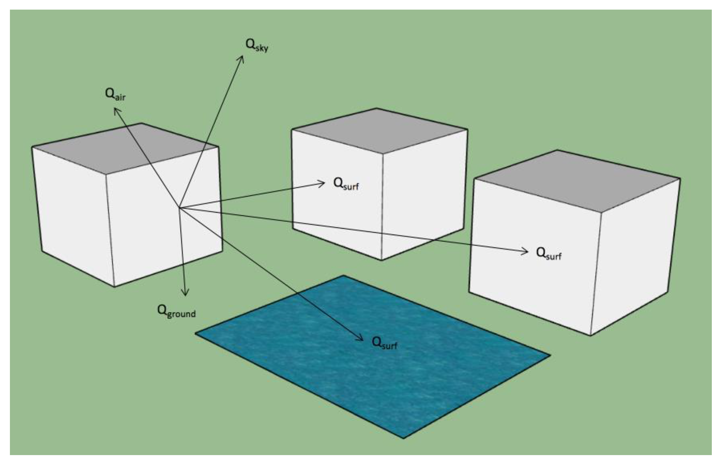
While the thermal performance of individual buildings is well documented in general building energy simulation tools, the thermal interactions between buildings are generally less understood or not considered [4]. In the urban context, radiant heat exchange occurs between buildings’ exterior surfaces and (1) the sky, (2) the ground, and (3) other surfaces, including other buildings’ exteriors surfaces, wetlands, vegetation cover, trees, etc. Among these, the thermal interconnections between buildings mainly occur via the longwave radiant (LWR) heat exchange between buildings’ exterior surfaces [5,6].

Literature has introduced the processes to simulate or measure the long-wave radiant heat exchange between buildings and their surrounding urban surfaces [7]. Urban sensing is one way to quantify heat transfer. Kwon and Lee [8] conducted measurements and collected data to investigate shifts in LWR over time, depending on spatial aspects, focusing on trees, buildings, and their sizes. The results demonstrated that a 50 % increase in tree volume induced a 10% decrease in mean radiant temperature (MRT). Ghandehari et al. [9] estimated the urban radiant heat transfer based on hyperspectral imaging of building blocks in Manhattan, New York. The study also introduced a geospatial radiosity model to describe the physical processes of LWR heat exchange between buildings. In this model, the urban geometry (building and street surfaces) is represented by a mesh of small surface “patches”. 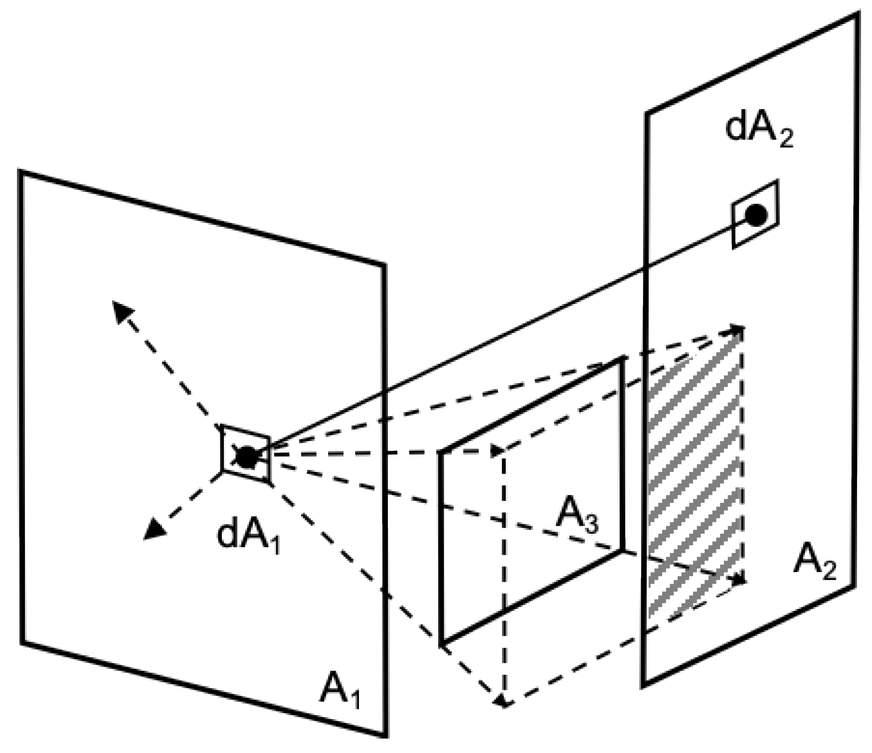Similar radiosity methods are commonly adopted in most urban microclimate simulations [10]. Among these simulation methods, view factors between urban surfaces are calculated by differential area view angle calculation [11] or Monte Carlo Ray Tracing (MCRT) sampling approach [12]. However, these studies within the urban microclimate domain lack granularity in building physics, including detailed geometries, system configurations, and physical processes (e.g., lighting, HVAC) inside buildings.

In urban building energy modeling, various approaches have been introduced to the treatment of external LWR exchange in urban energy modeling to simulate the thermal interactions between buildings. Algorithms and tools were developed to address the need for modeling building energy in an urban context, considering the surrounding buildings [7]. Urban building energy modeling (UBEM) tools have been developed to simulate an urban district considering energy flow between buildings for planning purposes. Evins et al. [13] coupled EnergyPlus with the microclimate tool, ENVI-Met, to improve the longwave exchange process of building energy modeling considering other building surfaces. The case study results indicated that the combined impact of the street canyon and shading devices led to an increase in the surface temperature of up to 6 ℃, a decrease in annual heating load of 18%, and an increase in the cooling load of 19%. A similar study by Miller et al. [14] included the LWR exchange as part of a co-simulation process of an urban scale simulation program, CitySim, and EnergyPlus. The LWR exchange between surfaces was computed in CitySim by a linearization of the energy balance using the temperature difference between surfaces and their environment. They then used functional mockup units (FMU) for coupling weather and load simulations, and the results indicate an up to 36% discrepancy in heating and 11% in cooling load calculations between individual and coupled simulations. However, both studies simplified the physical processes due to the limitation of the simulation engine and computing resources. The coupled physics also prevents the simulation from scaling up to apply the model in a larger urban domain.

EnergyPlus [15] is the U.S. Department of Energy’s flagship building energy software for simulating the dynamic energy and environmental performance of buildings. An EnergyPlus model calculates a building’s thermal loads, system response to those loads, and resulting energy use, along with related metrics like occupant comfort and energy costs. Applied to urban energy modeling, EnergyPlus calculates the overall thermal behavior of the urban buildings in terms of urban boundary conditions (i.e., exterior surface temperatures) and the heat and airflow exchange with the urban environment [16]. Yet in older versions, EnergyPlus models buildings as standalone entities and physical processes. Traditionally in EnergyPlus, calculations for LWR heat exchange between exterior surfaces and their surrounding surfaces were over-simplified, considering only the radiative heat exchange from and to the sky and the ground. However, in a dense urban setting with lots of high-rise buildings, these effects can be large and can have impacts on building energy and environmental performance. Thus, this simplification is causing potential under or over-estimate of buildings’ energy consumption and exterior surface temperatures. Explicitly considering the thermal interconnections between buildings in an urban context requires simulation engines to evolve to incorporate this new information into calculations and to do in a scalable way that achieves feasible computing performance and accuracy for urban scale applications.

Apart from the simulation engine to be involved, view factors between urban surfaces are also required to calculate the LWR heat exchanges in an urban scene. In radiative heat transfer, a view factor from surface A to B is the proportion of the radiation which leaves surface A that strikes surface B. The analytical calculation of view factors between urban surfaces is computationally expensive considering the complex urban geometry. Alternatively, ray tracing has been widely adopted to simplify the calculation. Ray tracing is a computer graphics algorithm originally proposed for generating photorealistic renderings by emulating the transmission of light rays in 3D scenes. In this algorithm, a large number of rays are shot from a source region into the scene, while the intersection between the rays and scene objects are then solved and used to recursively compute a path of the ray bouncing between object surfaces. Panao et al. used the ray-tracing method to determine the view factors in a 3D regular urban area by simplifying the urban block geometry [17]. The four vertical façades, the sky, and the ground are divided into parcels, and the estimation of the view factor matrix is calculated by shooting a large number of rays from each parcel with a random direction and tracking the surfaces they intersect. However, due to the limited computing resource, the parcels are divided coarsely in a large urban scene, and this sacrifices the accuracy when the scene is complex. Jones et al. have also presented a ray casting method of calculating view factors between two interior building surfaces on the basis of the geometric analogy algorithms [18,19]. To calculate a view factor from surface A to B, a Monte Carlo approximation is produced by selecting points on surface A and casting one ray from each point. The view factor is then calculated as the fraction of rays whose first intersection is with surface B. The approximation can also be used in calculating exterior surfaces’ view factors in an urban district scene. The simulation engines, such as EnergyPlus, can take advantage of these faster algorithms by integrating the external calculation results into urban building energy simulation.

This paper presents the feature implemented in EnergyPlus version 8.8 and later to improve its accuracy in an urban context by considering thermal interactions between buildings and expanding its applicability to urban scale building energy simulation. This paper also introduces a GPU-accelerated ray tracer for computing the view factors between large numbers of urban surfaces efficiently. The feature is introduced along with a case study of an urban district in the downtown Chicago area to demonstrate its use and impact. The study addresses the need for taking explicit consideration of the thermal interactions between urban surfaces in a dense urban setting with high-rise buildings. In urban-scale modeling applications, this new feature enables modeling the urban canyon effect, which also influences the building’s energy demand and indoor occupant thermal comfort. The study also demonstrated how modern computing architecture enables the massive amount of calculation required for considering buildings’ thermal interactions in urban energy modeling, and the potential to apply the algorithms in a larger spatial scale of urban building energy simulation and coupled multiscale urban systems.

2. Thermal Interactions between Buildings

2.1. Modeling Longwave Radiant Heat Exchange between Buildings in EnergyPlus

Old versions of EnergyPlus assumed that the temperatures of exterior surfaces of surrounding nearby buildings are essentially uniform and that longwave radiant exchange between them is negligible. With this assumption, the exterior surface heat balance equation was simplified as:

$${\mathrm{q}}_{\mathrm{LWR}}= \mathsf{\epsilon }\mathsf{\sigma }\left[{\mathrm{F}}_{\mathrm{sky}}\left({\mathrm{T}}_{\mathrm{sky}}^4-{\mathrm{T}}_{\mathrm{surf}}^4\right)+{ \mathrm{F}}_{\mathrm{a}}\left({\mathrm{T}}_{\mathrm{a}}^4-{\mathrm{T}}_{\mathrm{surf}}^4\right)+{ \mathrm{F}}_{\mathrm{g}}\left({\mathrm{T}}_{\mathrm{g}}^4-{\mathrm{T}}_{\mathrm{surf}}^4\right)\right],$$

(1)

where,

• $\mathsf{\epsilon }=\mathrm{longwave} \mathrm{emittance} \mathrm{of} \mathrm{the} \mathrm{surface},$
• $\mathsf{\sigma }=\mathrm{Stefan}-\mathrm{Boltzmann} \mathrm{constant} \left(\mathrm{W}\cdot {\mathrm{m}}^{-2}\cdot {\mathrm{K}}^{-4}\right),$
• ${\mathrm{T}}_{\mathrm{surf}}=\mathrm{Temperature} \mathrm{of} \mathrm{the} \mathrm{exterior} \mathrm{surface} \left(\mathrm{K}\right),$
• ${\mathrm{T}}_{\mathrm{sky}}=\mathrm{Sky} \mathrm{temperature} \left(\mathrm{K}\right),$
• ${\mathrm{F}}_{\mathrm{sky}}=\mathrm{View} \mathrm{factor} \mathrm{of} \mathrm{the} \mathrm{sky},$
• ${\mathrm{T}}_{\mathrm{g}}=\mathrm{Ground} \mathrm{temperature} \left(\mathrm{K}\right),$
• ${\mathrm{F}}_{\mathrm{g}}=\mathrm{View} \mathrm{factor} \mathrm{of} \mathrm{the} \mathrm{ground},$
• ${\mathrm{T}}_{\mathrm{a}}=\mathrm{Temperature} \mathrm{of} \mathrm{the} \mathrm{outdoor} \mathrm{air} \left(\mathrm{K}\right),$
• ${\mathrm{F}}_{\mathrm{a}}=\mathrm{View} \mathrm{factor} \mathrm{of} \mathrm{the} \mathrm{outdoor} \mathrm{air}.$

In particular, the outdoor air temperature component includes the longwave radiation to the particles, dust, and water vapors in the ambient air. The longwave view factors to the ground and sky are calculated with the following equations [20,21]:

$${\mathrm{F}}_{\mathrm{g}}=0.5\left(1- \cos \mathsf{\varphi }\right),$$

(2)

$${\mathrm{F}}_{\mathrm{sky}}=0.5\left(1+ \cos \mathsf{\varphi }\right)\ast \mathsf{\beta },$$

(3)

$${\mathrm{F}}_{\mathrm{a}}=0.5\left(1+ \cos \mathsf{\varphi }\right)\ast \left(1-\mathsf{\beta }\right),$$

(4)

where ϕ is the tilt angle (the angle between the Z-axis and the normal to the surface) in degrees of the surface, $\mathsf{\beta }$ is the sky and air radiation split factor defined by:

$$\mathsf{\beta } =\sqrt{ 0.5 \left(1+ \cos \mathsf{\varphi }\right)}$$

(5)

In many urban contexts, specifically in the presence of urban canyons—relatively narrow streets with tall, continuous buildings on both sides of the roads—this assumption is flawed in two aspects. First, in most urban areas, the view factors of a building façade to surrounding buildings’ façades are not neglectable, and the temperature of the surrounding façades can be much higher or lower than the sky or ground temperature. Second, at different times of a day, the individual building surface temperature can deviate each other to a couple of degrees Celsius due to different orientations [22]. As the north façade of a building often faces the south facades of surrounding buildings, under different circumstances, some exterior zones may be absorbing heat from longwave radiation, while other zones are losing heat to the ambient.

Considering this, we modified the EnergyPlus code to optionally explicitly consider the longwave radiant heat exchange to and from buildings’ nearby surfaces (i.e., surrounding buildings’ exterior surfaces, water bodies, green lands, etc.) in addition to the radiation from sky and ground as currently considered (Figure 1).

In the enhanced model implementation, the energy balance of an exterior building surface from the sky, air, ground, and surrounding surfaces is written as:

$${\mathrm{q}}_{\mathrm{LWR}}= \mathsf{\epsilon }\mathsf{\sigma }\left[{\mathrm{F}}_{\mathrm{sky}}\left({\mathrm{T}}_{\mathrm{sky}}^4-{\mathrm{T}}_{\mathrm{surf}}^4\right)+{ \mathrm{F}}_{\mathrm{a}}\left({\mathrm{T}}_{\mathrm{a}}^4-{\mathrm{T}}_{\mathrm{surf}}^4\right)+{\mathrm{F}}_{\mathrm{s}1}\left({\mathrm{T}}_{\mathrm{s}1}^4-{\mathrm{T}}_{\mathrm{surf}}^4\right)+{\mathrm{F}}_{\mathrm{s}2}\left({\mathrm{T}}_{\mathrm{s}2}^4-{\mathrm{T}}_{\mathrm{surf}}^4\right)+\dots +{ \mathrm{F}}_{\mathrm{sn}}\left({\mathrm{T}}_{\mathrm{sn}}^4-{\mathrm{T}}_{\mathrm{surf}}^4\right)+{ \mathrm{F}}_{\mathrm{g}}\left({\mathrm{T}}_{\mathrm{g}}^4-{\mathrm{T}}_{\mathrm{surf}}^4\right)\right],$$

(6)

where

• ${\mathrm{T}}_{\mathrm{si}}=\mathrm{Temperature} \mathrm{of} \mathrm{surrounding} \mathrm{surface} \mathrm{i} \left(\mathrm{K}\right),$
• ${\mathrm{F}}_{\mathrm{si}}=\mathrm{View} \mathrm{factor} \mathrm{of} \mathrm{surrounding} \mathrm{surface} \mathrm{i}.$

Each surface imports the externally calculated ${\mathrm{F}}_{\mathrm{si}}$. The modified Equations (7)–(9) are used to calculate the remaining view factor to the ground, sky, and air after partially obstructed by the surrounding surfaces. The sum of all view factors equals one, i.e., ${\mathrm{F}}_{\mathrm{sky}}+{{\displaystyle \sum }}^{ }{\mathrm{F}}_{\mathrm{si}}+{ \mathrm{F}}_{\mathrm{g}}+{ \mathrm{F}}_{\mathrm{a}}=1$.

$${\mathrm{F}}_{\mathrm{g}}=\left(1-{\displaystyle \sum }_{i=0}^n{\mathrm{F}}_{\mathrm{si}}\right)\ast 0.5\left(1 – \cos \mathsf{\varphi }\right),$$

(7)

$${\mathrm{F}}_{\mathrm{sky}}=\left(1-{\displaystyle \sum }_{i=0}^n{\mathrm{F}}_{\mathrm{si}}\right)\ast 0.5\left(1+ \cos \mathsf{\varphi }\right)\ast \mathsf{\beta },$$

(8)

$${\mathrm{F}}_{\mathrm{a}}=\left(1-{\displaystyle \sum }_{i=0}^n{\mathrm{F}}_{\mathrm{si}}\right)\ast 0.5\left(1+ \cos \mathsf{\varphi }\right)\ast \left(1-\mathsf{\beta }\right),$$

(9)

In EnergyPlus, the heat-balance Equation (6) is solved iteratively within each time step (ranging from 1 to 60 min), resulting in small updates to the surface and air temperatures until convergence criteria are met. Detailed heat and mass transfer processes are documented in the Engineering Reference of EnergyPlus [23]. To avoid the complexity of iterative temperature exchange, for surrounding surfaces, we use a fixed temperature T_si at the previous time step, assuming one timestep lag. This simplification may lose some fidelity (if a larger time step of 60 min is used in simulation) but significantly improves computing performance.

In the EnergyPlus simulation input, the exterior surfaces are described as input objects. To each exterior surface object, we assign a “surrounding surfaces” object, which declares a list of input fields including surrounding surfaces names, view factors, and surrounding surface annual temperature schedules. The temperature schedule can be overwritten at each time step via the co-simulation interface or using the EMS (Energy Management System) feature of EnergyPlus with co-simulation on an urban scale.

2.2. Modeling Urban Buildings and Their Surrounding Surfaces

We use the CityBES platform to model buildings in the urban context. CityBES is an open and free data and computing web platform which uses CityGML-based 3D city models to simulate building performance at the urban scale, adopting EnergyPlus and OpenStudio as its simulation engines [24]. CityBES models the neighborhood buildings as shading surfaces in EnergyPlus to consider the solar overshadowing effect between buildings [25]. Instead of calculating the view factor of each surface of the domain building to every surface of a surrounding building, we adopt the shading surfaces defined in CityBES as a building’s surrounding surfaces and calculate their view factors to each exterior surface for radiant heat exchange calculation including windows, walls, and roofs of each exterior zone. Figure 2 shows the 3D visualization of a building model along with its surrounding buildings (grey surfaces). Specifically, when the closest ground distance of the target building and a surrounding building is less than the height multiplier times the surrounding building’s height, the surrounding building may shade the target building, so the surrounding building is considered as a shading building for the target building. The height multiplier is calculated based on an average sun angle of a certain location as a simplification. In reality, the grey surrounding surfaces are composed of windows and walls from surrounding buildings, which have unevenly distributed temperatures. The simplification of considering the uniform surface temperature of a surrounding façade and a single view factor to it significantly reduces the computation needs.

2.3. View Factor Calculation

The double area integration formula is commonly used to calculate the view factors between two planar surfaces (i.e., surface A₁ & A₂), and the fundamental expression is written as:

$${\mathrm{A}}_1{\mathrm{F}}_{12}=\underset{{\mathrm{A}}_1{\mathrm{A}}_2}{\overset{ }{{\displaystyle \iint }}}\frac{\left({\mathrm{dA}}_1{\cos \mathsf{\theta }}_1\right)\left({\mathrm{dA}}_2{\cos \mathsf{\theta }}_2\right)}{{\mathsf{\pi }\mathrm{r}}^2},$$

(10)

where A₁ and A₂ (m₂) are the areas of surfaces 1 and 2; θ₁ and θ₂ (°) are the angles between the norms to surface differential elements dA₁ and dA₂ and the vector between those differential elements; r is the length of that vector [26]. This method is used in the View3D tool developed for evaluating radiation view factors between two 3D surfaces of interior surfaces in EnergyPlus. When a third surface is added between two planar surfaces, View3D calculates the blockage factor by tracing the rays between each two differential elements dA₁ and dA₂, represented as the shadowed area in Figure 3 [27]. The adaptation to the partial obstruction is less efficient in computing, and it cannot be used to calculate concave and curve surfaces as well.

To calculate the view factors between surfaces with more complex geometries at an urban scale, we developed a ray tracing technique to evaluate the double area integration formula. The raytracing algorithm performs Monte Carlo sampling by shooting rays between random points drawn from a pair of exterior surfaces. Each ray and its terminal points represent a discrete analog of the pair of differential area $\mathrm{d}{\mathrm{A}}_1$ and $\mathrm{d}{\mathrm{A}}_2$ in Figure 3. The ray tracer will then determine whether each ray can reach its target surface without hitting a third surface. The view factor from A₁ to a target surface A₂ can be then deduced as a sum of the $\frac{\cos {\mathsf{\theta }}_1\cos {\mathsf{\theta }}_2}{\mathsf{\pi }{\mathrm{r}}^2}$ terms over all surviving rays subject to proper normalization. Compared with the traditional analytical solutions and geometry analogy algorithms introduced in the literature review, the view factor tracer we developed carries the following advantages:

1. Rays are always directed between a pair of surfaces;

2. The obstructed surfaces are considered automatically;

3. The intersection of rays with many geometric objects can be solved analytically. This allows for efficient and robust handling of objects with non-convex and other complex shapes.

4. The computation for tracing individual rays is strictly independent and hence could be parallelized easily using GPU.

Our ray tracing program is written in CUDA C++ and makes use of the NVIDIA Optix Prime library. CUDA C++ is an extension of the C++ language with syntactic features for executing codes on the CUDA GPUs. Optix Prime is a lower-level program engine that simplifies the design of ray tracing applications that executes on either CUDA GPUs or x86 CPUs. Specifically, we used Optix to compute the point of intersection between rays and urban surfaces, while our custom CUDA C++ code handles scene modeling, ray generation, result consolidation, and post-processing. A table of view factors from all exterior surfaces to all surrounding surfaces is produced by the tracer to be imported in EnergyPlus calculations.

3. Case Study

3.1. Simulation Settings

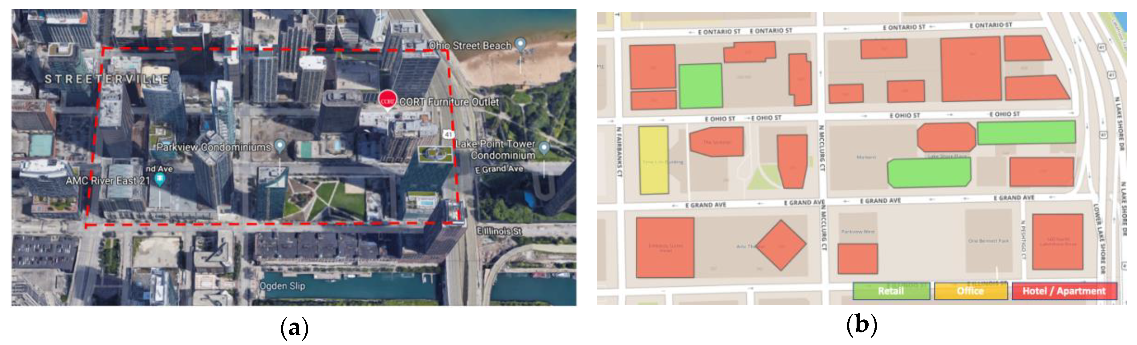
We chose a city block in the Chicago downtown area near Michigan Lake with highly dense high-rise buildings to conduct a case study, as shown in Figure 4. The selected district is in the downtown Chicago (LOOP) area, with a total of 22 buildings, as visualized in Figure 4a. The district is mostly composed of mix-used buildings, ranging from 3 to 60 floors. The highest building in the chosen area has 58 floors in total, and the lowest has 5 floors. Modeling the buildings in EnergyPlus, we simplified the urban building representations in two ways: (1) for mix-used buildings, the dominant usage is considered as the building type; (2) for high-rise towers with a podium that is used as garages, we only consider the tower part in the modeling. Figure 4b draws the footprint of buildings in the district, colored by their dominating building use type. Among the 22 buildings, 18 are large high-rise hotels, three are low-rise retail buildings, and one is a large office building. The newest construction was completed in 2013, and the oldest was built in 1968.

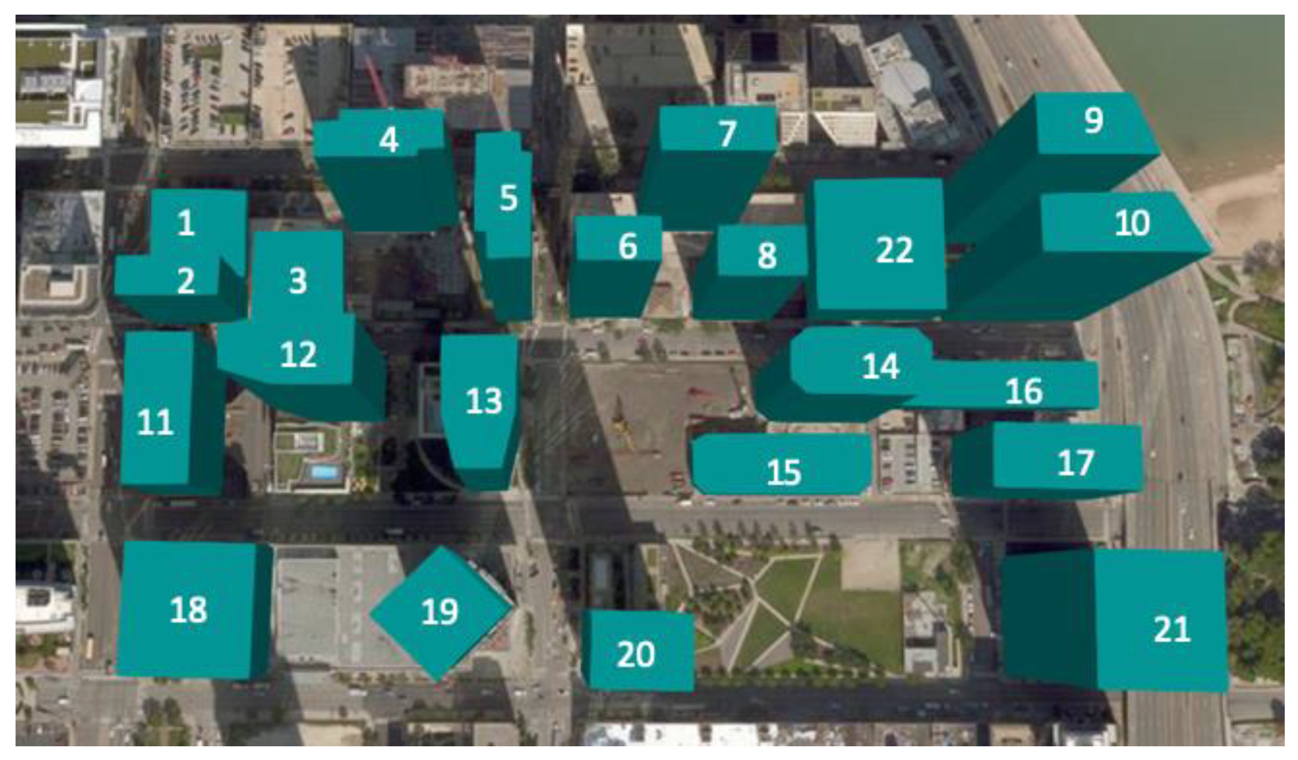
We then use CityBES to generate the EnergyPlus models for building energy simulation with the district buildings’ geographic and geometry information as input. CityBES models each building as an extruded polygon according to the building’s number of floors and height and applied zoning automatically based on the building footprint and building use type [28]. The models then infer detailed building systems and energy efficiency levels (e.g., insulation of envelope, lighting systems, HVAC systems, and equipment efficiency) based on the local building energy code of that particular year of build. The HVAC system types and efficiency levels are determined based on ASHRAE standard 90.1 [29]. Figure 5 is the CityBES visualization of the models, labeled with building IDs to facilitate further discussion.

With the simulation set up, we follow the listed steps to conduct the case study, and the results are presented accordingly.

1. Pre-scanning the text input files of each EnergyPlus model’s geometry data to extract the coordinates of the exterior wall, windows, roofs, and surrounding surfaces to generate ray-tracing scenes for the tracer and calculating the view factor of exterior surfaces of these 22 buildings.

2. Running each EnergyPlus building model individually and independently without considering inputs from other buildings, and output their hourly exterior surfaces temperature for a whole year.

3. Collecting each building’s hourly surrounding surface temperature schedules for a whole year from the simulated exterior surface temperatures in Step 2, using the weighted average temperature (by surface area) of each façade and roof.

4. Re-running each building model taking surrounding surfaces temperature schedules and their corresponding view factors to each exterior surface.

3.2. View Factors to the Surrounding Surfaces

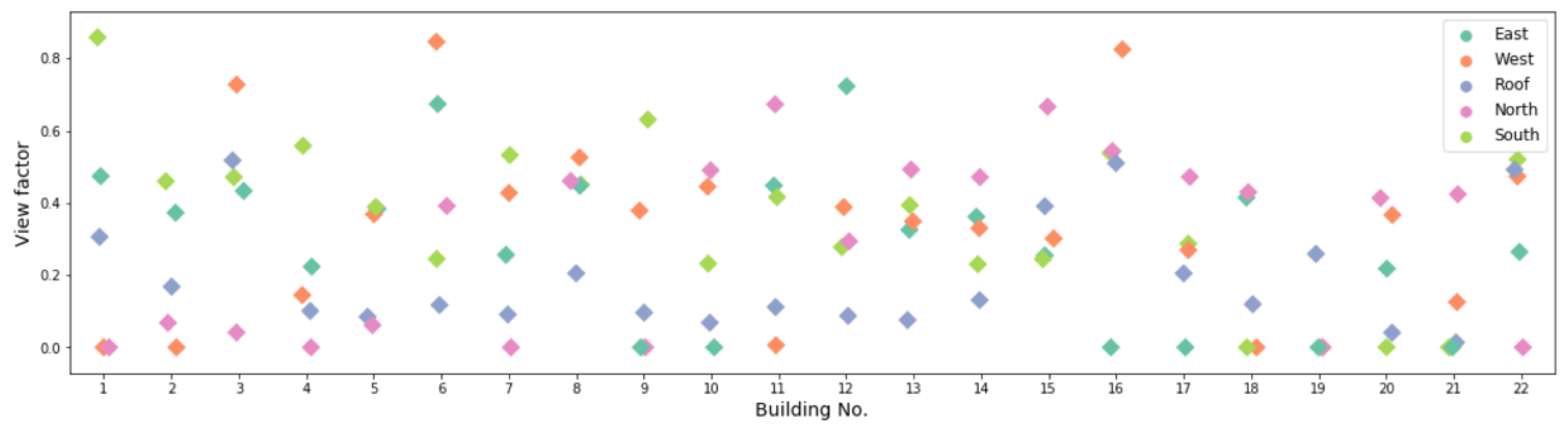
Averaging all surfaces on a façade, Figure 6 plots the average view factors of the four façades and the roof to surrounding surfaces of each building, calculated by the ray tracer we introduced.

Among the mixed low-rise and high-rise buildings in the studied dense urban district, lots of them have an average view factor of over 0.5 for at least one façade, and the largest view factor for one façade can be up to 0.8. This indicates these buildings are mostly shadowed, viewing less to the sky and ground than standalone buildings. Moreover, buildings of different geometries and locations view their surrounding buildings differently. For example, building 13 and 14 at the central part of the district are almost equally shadowed from the four façades, while buildings at the peripheral parts of the district usually have asymmetric view factors between opposed orientations. For the low-rise buildings such as building 3 and 16, their roofs’ view factors to the surrounding high-rise buildings can be over 0.5. As roofs usually contribute the most LWR heat gain or loss to the sky, how these heat exchanges can differ with the surrounding high-rise building shadowing effects should be discussed.

3.3. Thermal Behaviors of Building Exterior Surfaces

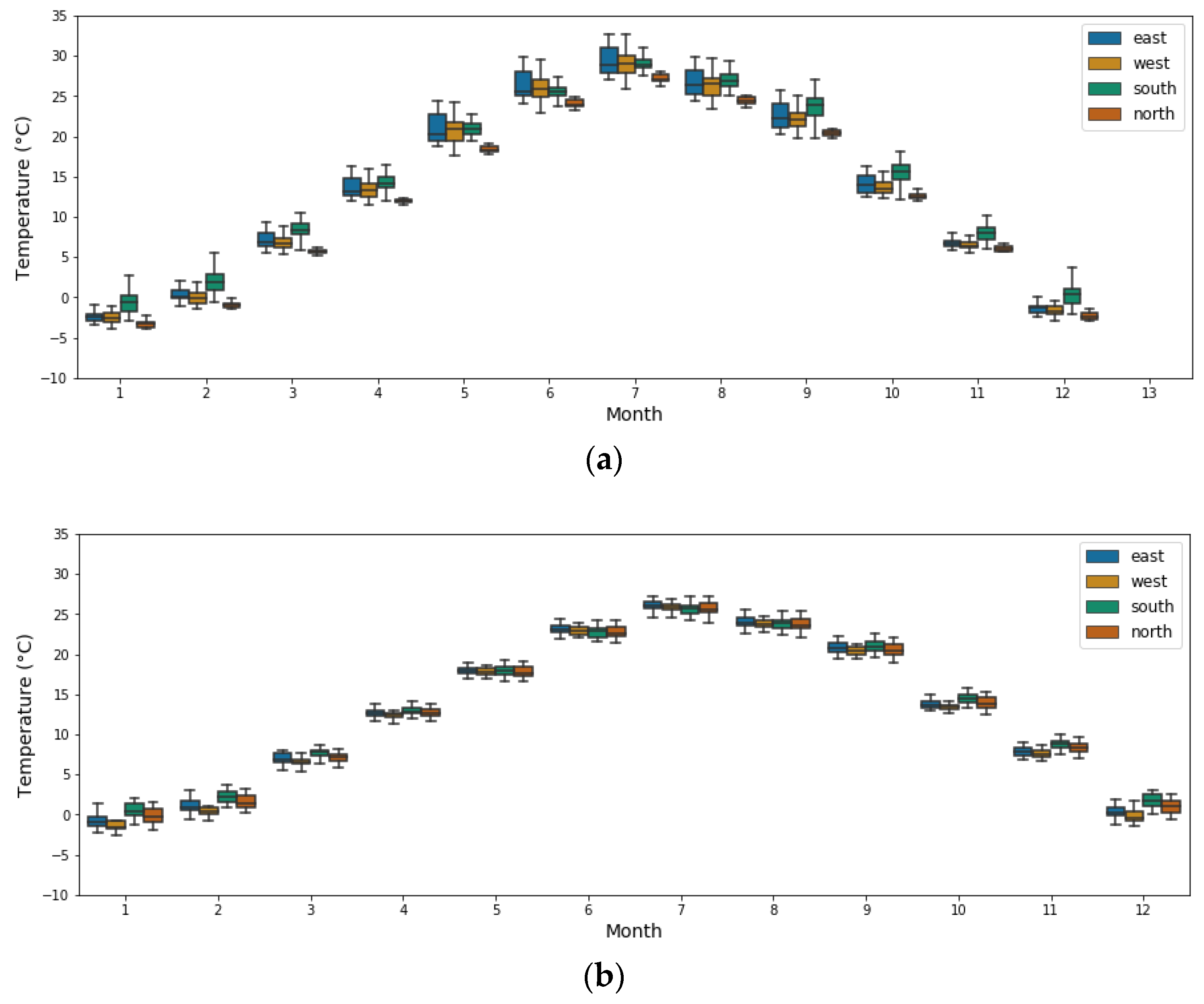
In different seasons of a year and different times of a day, the amount of solar radiation received by the four facades of buildings varies. We compared the monthly average exterior surface temperature, as shown in Figure 7, separating walls and windows. Each box plots the range of surface temperatures among all 22 studied buildings, with outliers neglected.

Located in the northern hemisphere, throughout the year, the exterior wall temperature of the south façade can be 2–5 °C higher than that of the north façade. The highest temperature differences appear during the fall and winter seasons, and during these times, the south-faced facades also see a larger temperature range of up to 8 °C between buildings. Monthly average temperatures of the east and west-faced walls are close during the winter season, while during summer, east façades observe a higher temperature on average. More significantly, from April to October, the thermal behavior of the walls facing east and west varies greatly among different buildings in the district, considering the varying shadowing effect of their facades. For window surfaces, the temperature variations among different orientations and buildings are lower, due to windows having considerably lower thermal absorptance to the solar radiation.

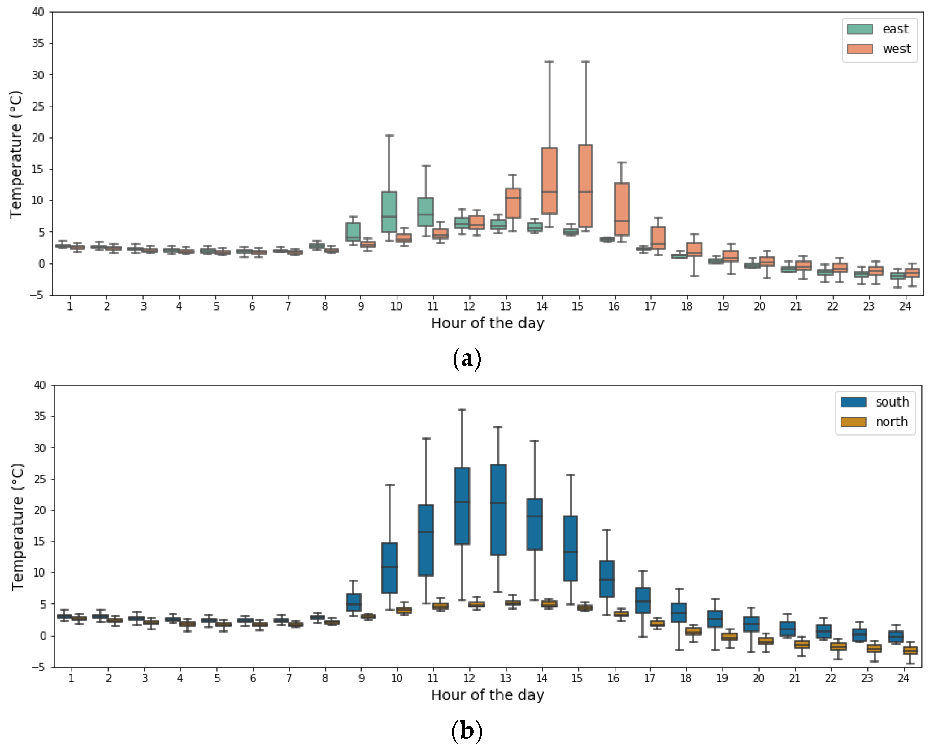
In Figure 8 and Figure 9, we picked January 21st and July 21st as a typical winter and summer day, respectively, and compared the hourly exterior wall temperatures, averaging each facade. Due to the daily variation of the sun position angle along with the shading effect from surrounding buildings, the surface temperature of different facades peaks at different hours of the day. In winter, the highest average temperature of the east, west, and south facades was observed at 11 am, 3 pm, and 12 pm, respectively. Although different buildings have a significant variation in surface temperature throughout the day, we still observe quite notable temperature gaps between opposed orientations on average. For east and west walls, the largest gap appears in the afternoon, when west facades have over 5 °C temperatures higher than the east ones. At noontime, the south facades with the largest view angle to the sun, observe a 15 °C higher surface temperature than the north facades, which benefit the least from the solar radiation during winter.

On the typical summer day, similarly, the average temperature of the east, west, and south facades peaks at 10 am, 3 pm, and 12 pm. The largest temperature difference appears in the morning between the east and west-faced walls. Comparing to the winter day, the temperature differences between north and south façade at noon, and between east and west façade in the afternoon are less substantial, while still showing a 5–10 °C gap correspondingly.

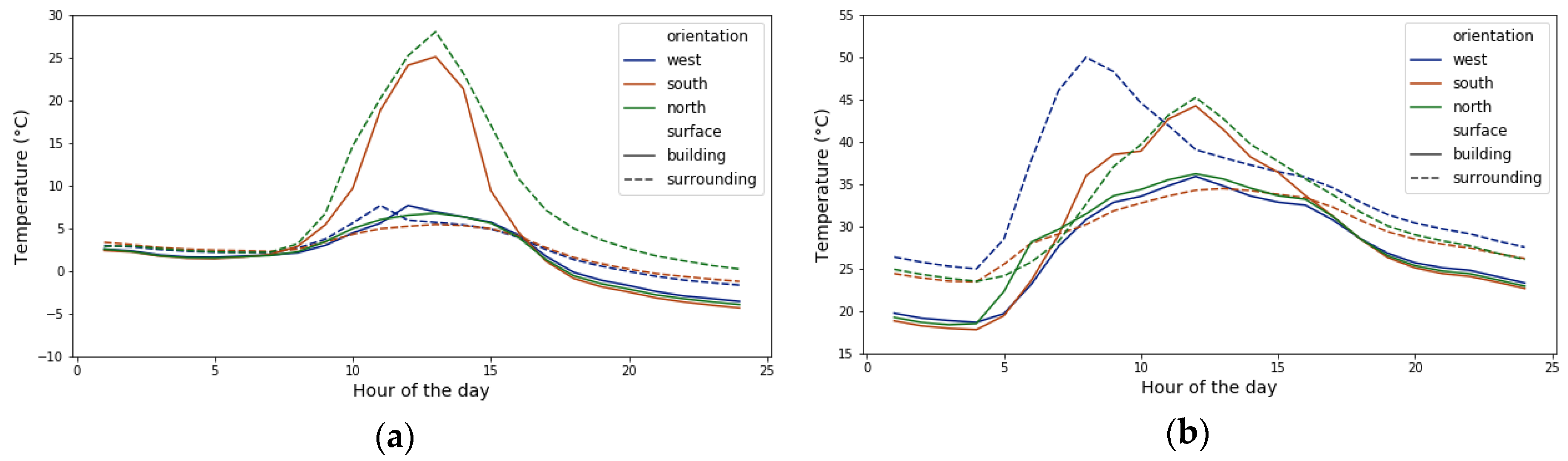
This triggers the temperature deviation from one façade to its surrounding surfaces facing opposite directions in the studied urban area. Figure 10 gives an example by plotting the average wall temperature of the west, south, and north facades of building 16, as well as these three facades’ surrounding surface temperatures. At noontime, the surface temperature on the south façade reaches up to 20 °C and 10 °C higher than its surrounding surfaces in winter and summer, correspondingly. The north façade shows the opposite behavior. With the temperature deviation, the north orientated surfaces absorb longwave radiant heat from surrounding buildings, while the south-orientated surfaces lose heat to the ambient. In the meantime, the west façade also shows up to 20 °C hotter than its surroundings in summer mornings, while in winter the effect is minimal.

3.4. Energy Impact Analysis

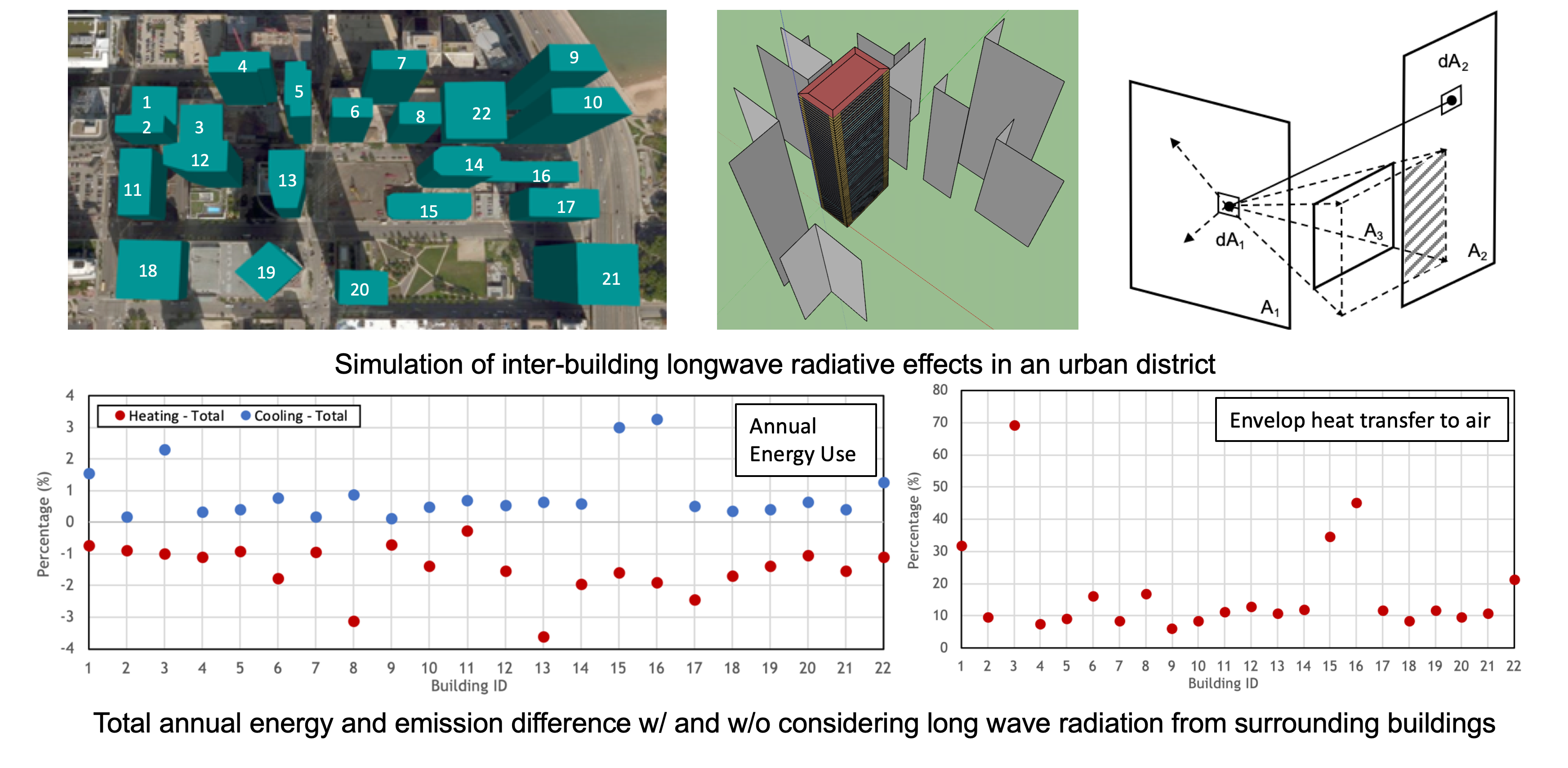
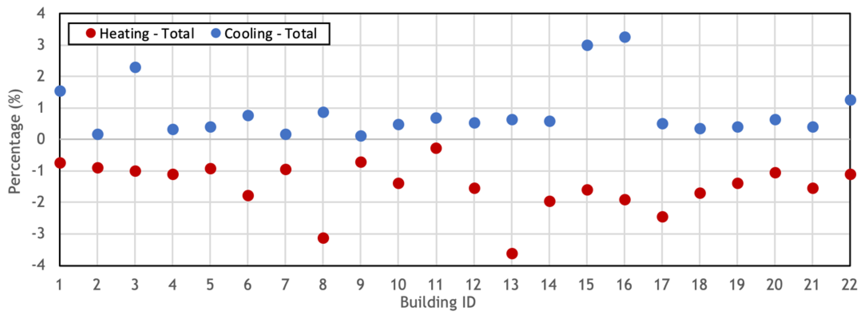
Following the above-mentioned steps, we ran simulations for the second round, taking account of the surrounding surfaces with their temperatures simulated from the first round. Figure 11 plots the total cooling and heating energy use differences in percentage when considering the LWR impact. Overall, most buildings have a greater decrease in heating load of over 1% than their increase in cooling load. We observe two particular energy behaviors of the buildings with the impact of the various LWR from surrounding buildings they received.

For cooling, the five low-rise buildings in the dense urban district we modeled show a greater energy demand increase than others. In particular, building 3 has the largest cooling load increase of 2.3% as a flat building surrounded by high-rise buildings in every orientation.

For heating, building 8, 13, and 17 show the greatest demand decrease, as their north facades are all largely shadowed by a south-faced surface with high radiant temperature, considering the exterior wall temperature gap between north and south façade can be up 15 °C. Building 8 has the largest heating load decrease of 3.2%. However, this effect does not apply to buildings 10 or 11, as although they both have a large view factor at the north side, the surrounding surfaces viewed by their north façades are also greatly shadowed, thus the influence of temperature gaps is mitigated.

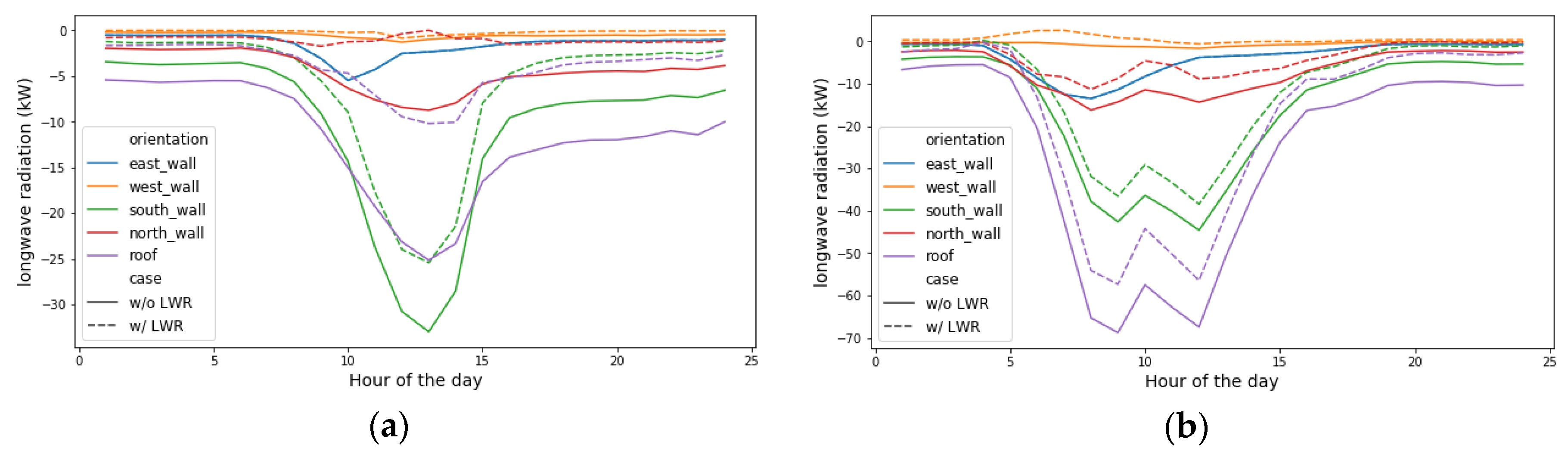
To further illustrate this, we compare the net thermal radiation heat gain rate for each façade for building 16 as an example in Figure 12.

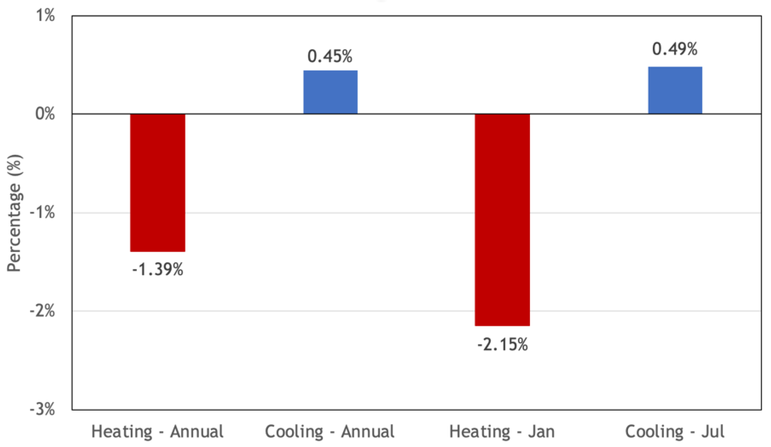
For each building, the heating energy decrease in winter and cooling energy increase in summer generally offset, resulting in a less considerable total energy consumption difference annually. For the district (Figure 13), the total heating and cooling energy differences are −1.39% and 0.45% for the annual simulation and are −2.15% and 0.49% for January and July in total.

3.5. Environmental Impact Analysis

We further analyzed the environmental impact of the surrounding surfaces LWR effect in terms of exterior surface temperature increase. The increased temperature of urban surfaces contributes to the increased heat transfer through convection and LWR to the ambient air. As building exterior surfaces in EnergyPlus originally view their ambient as partial sky and partial ground, adding the LWR effects from surrounding surfaces with a much higher temperature than the sky or ground, extra heat is added to the surface heat balance calculation. 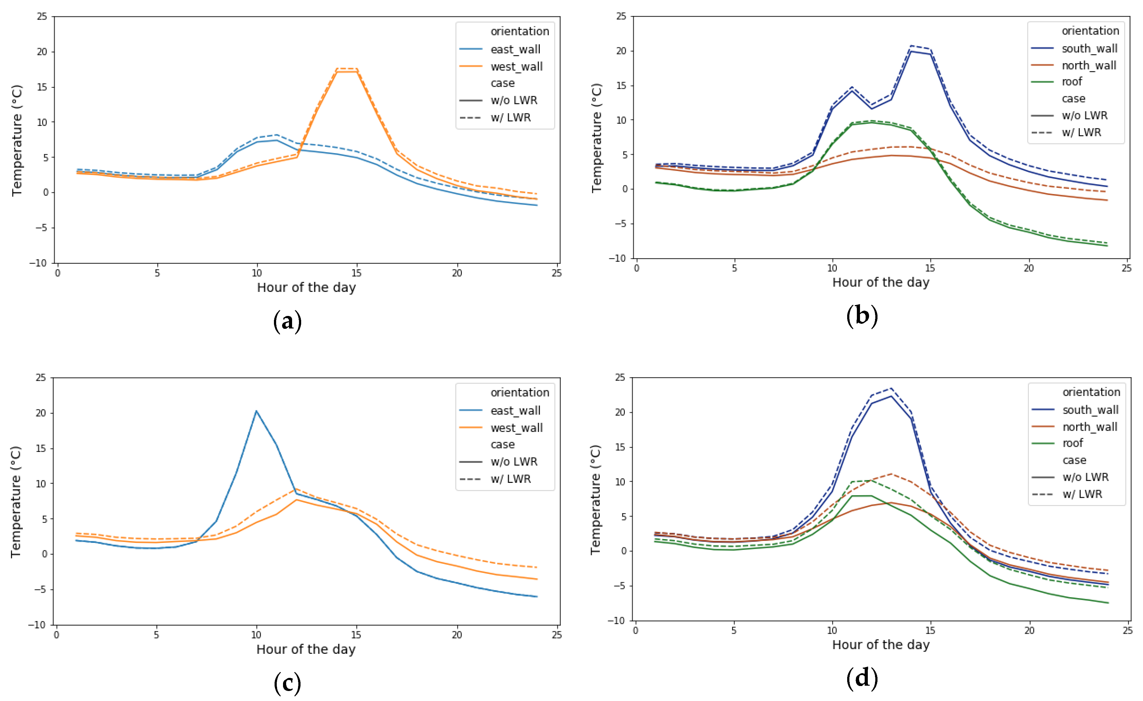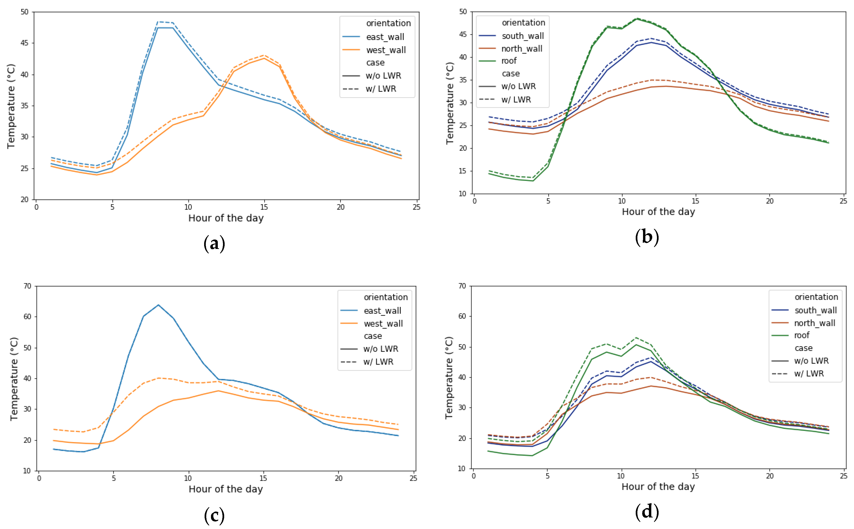Figure 14 and Figure 15 demonstrate this effect on building 13 and building 16.

In winter, for the low-rise building 16, the LWR effect lifts the north-facing surface and roof temperature to around 5 °C and 3 °C at 1 pm. The effect is less notable in the high-rise building 13, where the surface temperatures of the west and north facades are around 1–2 °C higher considering the LWR effect.

On the typical summer day, the amount of temperature lift on the north façade and roof is similar to that in winter, while the peak time shifts to 11 am. A more significant temperature shift appears at the west wall temperature in the early morning for building 16, reaching up to 10 °C, when the opposing west facade of building 14 has the greatest LWR impact.

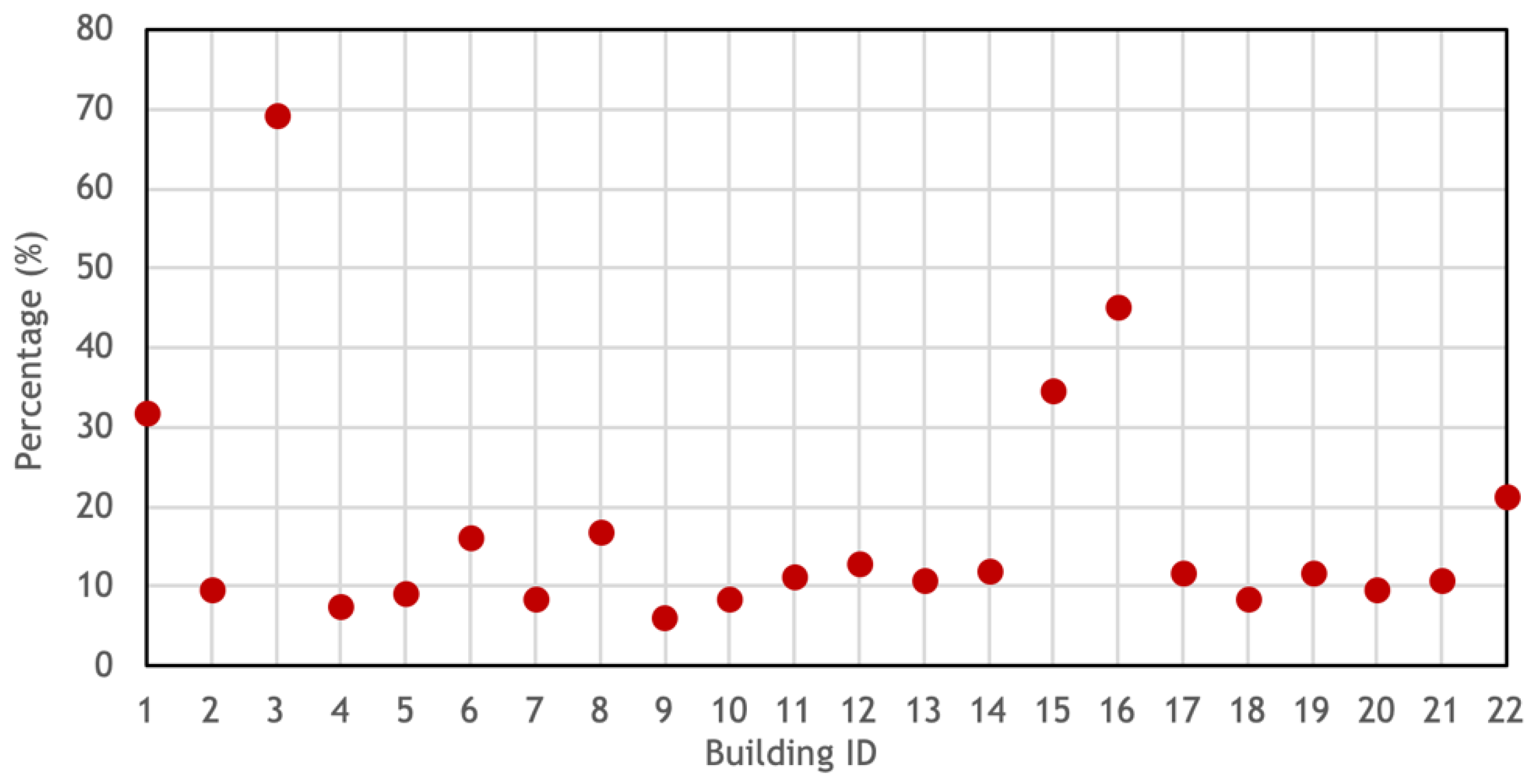
Due to the rise of the surface temperature, the heat transfer from exterior surfaces to the ambient air through convection and LWR also increases. As plotted in Figure 16, the difference is approximately 10–20% for the annual accumulated heat loss to the ambient air from most of the buildings, and the total increase at the district level is 11.6%. For the five low-rise buildings, in particular, the increase is remarkably higher, contributed by the roof temperature increase.

It is worth considering how this deviation influences pedestrian level thermal comfort. Moreover, it served as the boundary conditions of the urban microclimate, building facades’ thermal behaviors at different orientations should also be taken into consideration in detailed urban canopy models.

4. Discussion

The results show the thermal interactions between buildings should not be neglected when some surfaces of a building are surrounded by other buildings’ surfaces which receive a great amount of solar radiation and have significantly higher surface temperatures. A low-rise building surrounded by high-rise buildings is an example of this effect, as the roof and facades of four orientations are all radiated by urban surfaces with a higher temperature than the sky, air, or ground. The shadowing effect between two urban surfaces, in general, mitigates this impact, as when surfaces are mostly shaded, the timely and seasonally temperature differences between the two surfaces are not obvious throughout a year.

However, this case study may not unveil all aspects of this effect. First, the study does not consider the thermal exchange with urban objects such as trees or shading by trees; Second, each façade is treated as a lump surface with a uniform temperature in considering its LWR impact on surrounding surfaces. In reality, the façade has many surfaces with different temperatures and view factors to surrounding surfaces; Third, the studied area consists the most of hotel and apartment buildings. A larger community with more diverse building types and configurations may demonstrate varied energy behavior, as the energy demands peak at different times of a day. Moreover, it is also worth considering the irradiation trapping effect by conducting the case study iteratively, updating the exterior surface temperatures at every iteration until they converge. A finer coupling resolution with data exchange hourly or daily is required for this analysis, and a coupled simulation architecture may help facilitate it.

Overall, the study introduced an approach to considering LWR from surrounding surfaces explicitly in urban building energy modeling using the EnergyPlus simulation engine. The term was neglected due to the complexity of calculating the view factors and temperatures of the surrounding surfaces. Comparing to the literature, the case study results indicate the radiant heat exchange between buildings has varying impacts on buildings’ cooling and heating energy demand and exterior surface temperature, which in turn can intensify the heat stress in the urban microclimate environment. Comparably, the case study includes details of the variation of the building types, geometries, and layouts as the representation of a real building district, and the results show different levels of energy demand changes to individual buildings, reflecting more granularity of the long-wave radiation impact.

Future work includes implementing the thermal interactions in an urban building energy modeling platform, such as CityBES, for simulation of the urban building performance. View factors of surrounding surfaces will be pre-calculated altogether using the ray tracing tool and stored for simulation use. The platform would allow studying more districts with different density and locations. More simulation at a higher fidelity and a large spatial domain would allow investigating the coupling resolution and its influence on accuracy. Furthermore, coupled simulation with urban microclimate and climate models allows quantifying the impact on pedestrians’ outdoor thermal comfort and how the irradiation trapping and increased urban surface temperature contribute to the UHI.

5. Conclusions

This paper presents a new feature implemented in EnergyPlus version 8.8 and later to improve its use for building energy modeling by considering the longwave radiation effect between buildings’ exterior surfaces. A case study was conducted within a city block in the Chicago downtown area with 22 highly dense mixed-used buildings. Results indicate the temperature difference between each building façade and its surrounding surfaces with opposite orientations leads to significant radiance heat exchange between building exterior surfaces. Results also show that this temperature gap between building surfaces and their surrounding building surfaces causes the net thermal heat gain of a building from its surrounding buildings, which induces the variations in exterior surface temperature, building loads, and energy use. In particular, for the studied district located at the mid-latitude area in the northern hemisphere, the longwave radiation from the surrounding surfaces to the roof accounts for most cooling demand increase, and that to the north façade accounts for most heating demand decrease.

The study addresses the need for taking explicit consideration of the thermal interactions between urban surfaces in a dense urban setting with high-rise buildings. More detailed quantification and validation of the effects of building interactions at a larger scale can improve the accuracy of urban building energy modeling.