Article

Generalized Modeling of Soft-Capture Manipulator with Novel Soft-Contact Joints

1
Beijing Key laboratory of Intelligent Space Robotic Systems Technology and Application, Beijing Institute of Spacecraft System Engineering CAST, Beijing 100086, China
2
School of Automation, Beijing University of Posts and Telecommunications, Beijing 100876, China
3
Suzhou Institute of Biomedical Engineering and Technology, Chinese Academy of Sciences, Suzhou 215163, China
*
Authors to whom correspondence should be addressed.
Energies 2020, 13(6), 1530; https://doi.org/10.3390/en13061530
Submission received: 12 February 2020 / Revised: 18 March 2020 / Accepted: 20 March 2020 / Published: 24 March 2020

Abstract

:
The space-borne manipulator has been playing an important part in docking tasks. Docking collision can easily lead to instability of both the manipulator and floating base. Aiming at the problem of soft capture, a novel soft-contact joint with dual working modes is developed, especially to buffer and unload the spatial collision momentum. Furthermore, considering a series-wound soft-capture manipulator with multi-joints, a generalized modeling method was established by using the Kane approach. Both the benefits of soft-contact joint and the effectiveness of dynamics equations are verified in MATLAB and Adams software by simulations of a two-joint manipulator with eight-DOF. The comparative simulation results showed the advantages of the proposed soft-contact joint in reducing instability from spatial impact.

1. Introduction

Target capture is an important part of the on-orbit service mission. Disturbances introduced by docking collisions may destabilize the manipulator and floating base. Realizing the soft contact of spatial on-orbit capture is of great significance to avoid basal instability and angular momentum transient overrun.
At present, the technology of spatially soft capture based on a spatial docking mechanism has achieved a lot, such as the cone-rod docking system, spatial flying net technology, electromagnetic docking, etc. [1]. In recent years, the spatial docking mechanism is still a research hotspot of many scholars. Feng [2] developed a new type of end effector prototype by combining the tendon-sheath transmission system with steel cable snaring mechanism. Olivieri [3] proposed a new docking mechanism that provides the basis for the connection and separation of small spacecraft in space. The Center for Space Research and Activities (CISAS) of the University of Padua developed the Autonomous Rendezvous Control and Docking Experiment (ARCADE), which is well-tolerated by non-nominal docking conditions, designed to have the ability of soft contact [4,5]. Liu [6] designed a variable topology 3-RSR polyhedron docking mechanism and has verified the practicability of the structure. Zhang [7] discussed the influence of the parameters of the docking mechanism for the soft contact of micro/small satellites. Li [8] proposed a feasible docking mechanism based on the noncooperative target docking technology points and verified its effectiveness through simulation analysis. In order to minimize the collision risk during docking and capturing of the tumbling target, Liu [9] put forward a noncontact method based on the eddy current effect to transmit the control torque to the tumbling target.
The above research on the space docking mechanism mainly focuses on the development of the capture mechanism end-effect device, as well as the contact mode and contact strategy research, but the manipulator was not employed as part of the docking mechanism. The manipulator is a key component of the space-borne arrest mechanism. In this regard, some scholars have studied the momentum, angular momentum, and the trajectory planning of the space-borne capture mechanism.
Beginning from momentum and angular momentum, Yoshida [10,11] first proposed the concept of a generalized inertia tensor (Ex-GIT) and virtual mass and used it to minimize the impact. Wee et al. [12] proposed the gradient projection method, which simultaneously minimizes the impulse generated by trajectory tracking and post-planning contact. Nenchev and Yoshida [13,14] adopted the reaction zero-space method to transfer the angular momentum of the post-collision base to the manipulator from the angle momentum, while using the joint damping control method to reduce the joint velocity and ensure base posture stability after spatial collision. Cong and Sun [15] proposed "straight arm grabbing", which is the most ideal state, but it is difficult for planar robots to achieve. Considering the direction of the tumbling movement along any arm, Oki [16] stabilized the tumbling target satellite by using time-optimal control of the free-floating robot. Based on the dual-arm sport robot, Guo et al. [17] calculated the pre-impact configure to minimize the effects of impacts on the robot’s angular momentum by use of the particle swarm optimizer. Chen et al. [18] put forward a motion-planning method for space robotic systems keeping the bases inertially fixed while performing on-orbit services, using a combination of point-to-point planning and a balance-arm. Xu et al. [19] proposed a dual-arm coordinated “area-oriented capture” (AOC) method to capture a noncooperative tumbling target, which has larger pose tolerance and takes shorter time for capturing a tumbling target.
In the aspect of acquisition mechanism trajectory planning, a robust adaptive controller is used to design the active controller to suppress the impact caused by spacecraft drift in [20]. Xu [21] studied the kinematic redundancy of flexible redundant manipulators; Larouche [22] adopted a motion-prediction control scheme for autonomous acquisition tasks. McCourt [23] investigated the use of model-based predictive control for the captures of multi-degree-of-freedom objects moving in a predictable manner. By combining reaction zero-space methods and particle swarm optimization algorithms, Zhang [24] studied a manipulator trajectory plan by adjusting the pose of the robotic arm and minimizing the attitude disturbance of the base. However, due to the inevitable existence of model errors and operational precision, it is impossible to fundamentally avoid the impact and disturbance caused by the capture process, and it is difficult to suppress the complex vibration after docking.
Recently, the realization of soft contact of spatial docking through novel vibration suppression approaches has attracted more and more attention. Chu [25] established a variable stiffness actuator and proposed a self-learning soft-grasp control algorithm to minimize the angular momentum of the base. Nguyen [26] applied the controllable MR damper [27] to a planar two-DOF manipulator for spatial capture, but the spatial collision problem is not resolved. In addition, Yu et al. [28] investigated spatial dynamics and control of a six-DOF space robot with flexible panels and considered the spatial impact problem, which indicates that flexible panels have a big influence on impact dynamic characteristics. Bian [29,30] applied an effective shock absorber to unload the nonlinear vibration of the manipulator based on the principle of internal resonance. However, to our best knowledge, few literatures mention designing novel joint structures for soft capture.
Motivated by the above observations, this paper attempts to design a novel joint with a decoupled damper and proposes a generalized modeling method for a serial capture manipulator with multi-stage damping. The main contributions are listed as follows:
(i) Based on the cross shaft, decoupled damper, and clutch switching, a novel soft-contact joint with dual working modes is developed, especially to buffer and unload the spatial momentum from capture.
(ii) A generalized modeling method for the space-borne soft-capture manipulator with multi-joints was established by using the Kane approach, and the simulation results showed the effectiveness of the proposed soft-contact joint in reducing instability from docking collision.
The rest of this paper is organized as follows. In Section 2 and Section 3, a soft-contact joint is developed by adding decoupled dampers. Section 4 gives the dynamic equations by using the Kane approach. In Section 5, the collision dynamics simulation for a two-joint manipulator with eight-DOF, was performed by a simulation of MATLAB and Adams software.

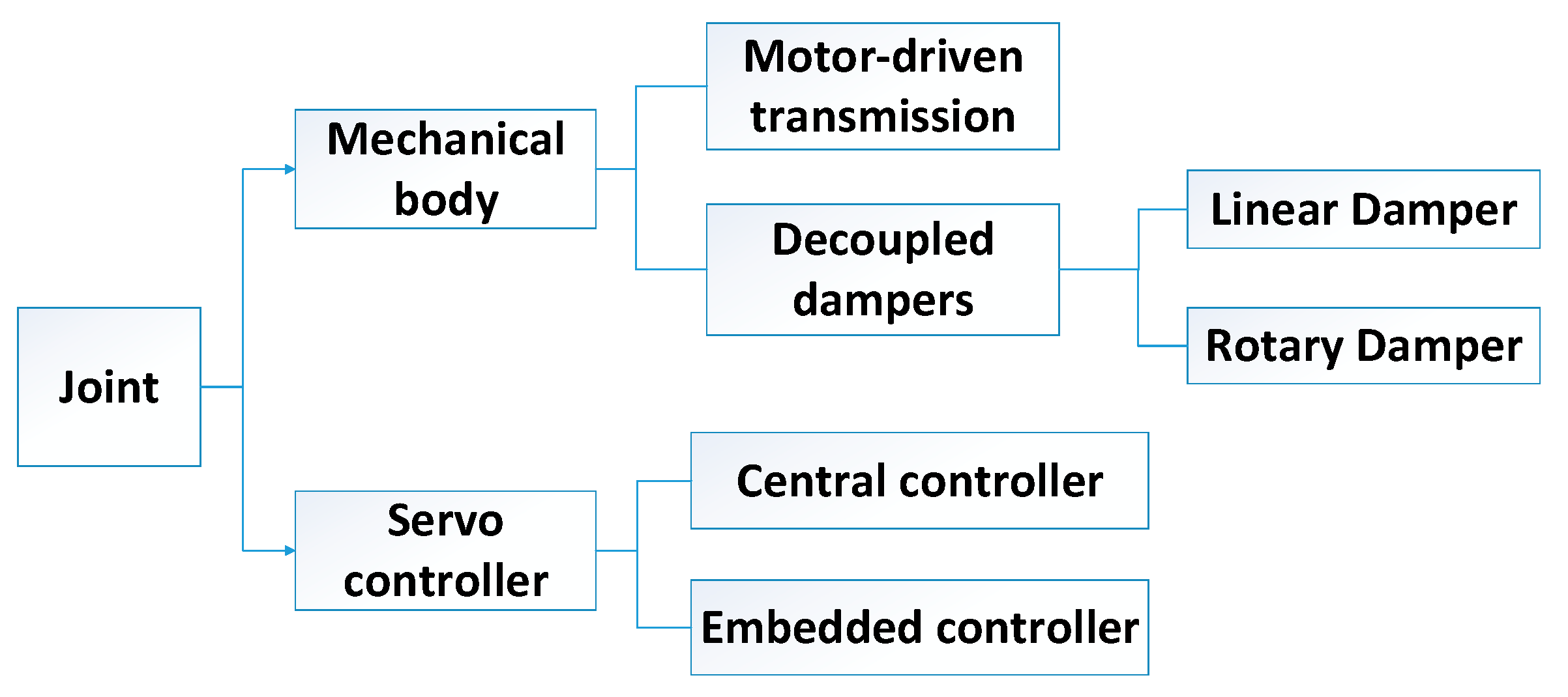
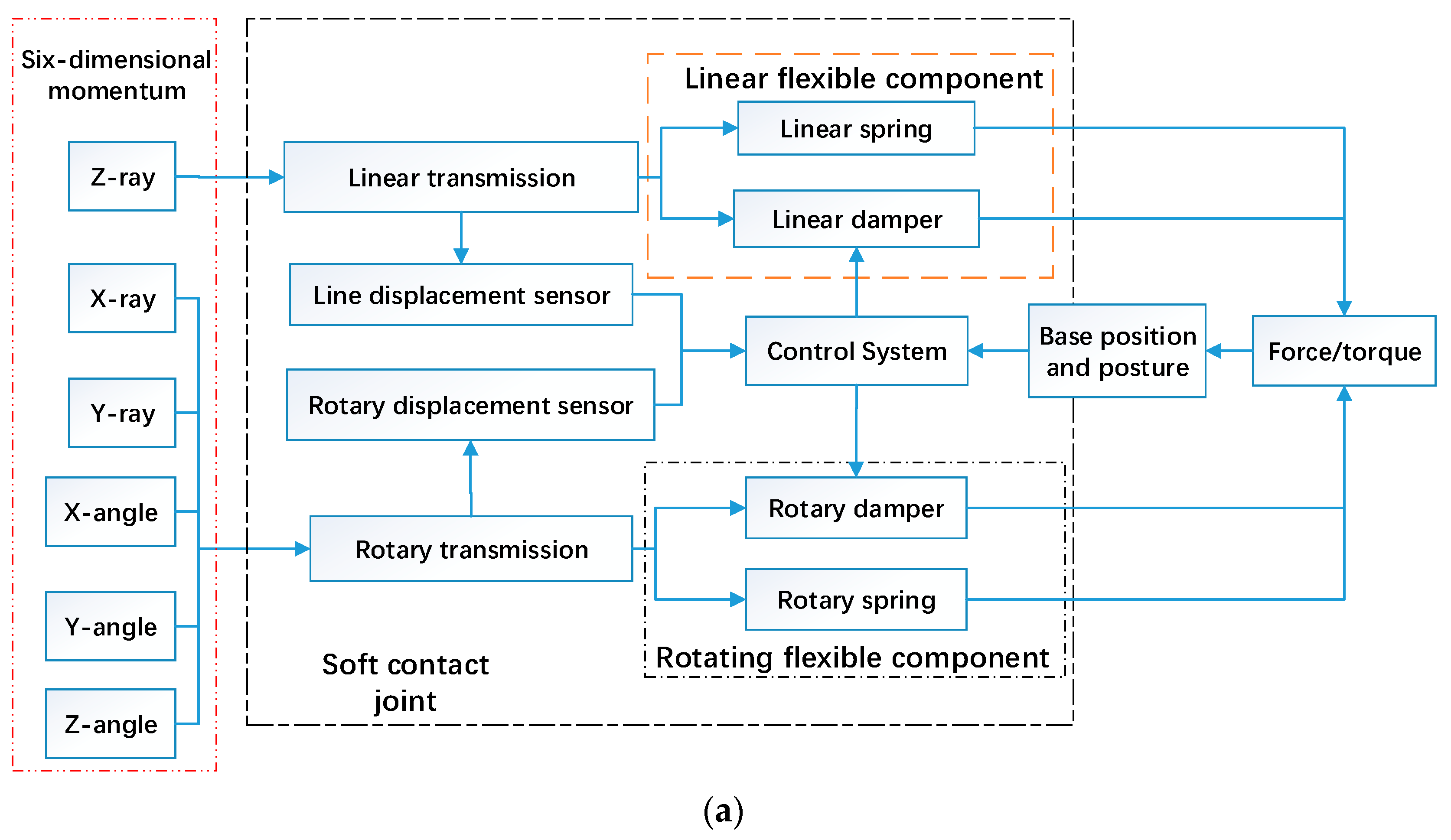
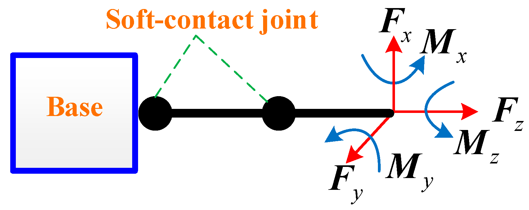
2. Joint Function for a Space-Borne Soft-Capture Manipulator

A soft-contact joint structure for a soft-capture manipulator is proposed. The 3D model of the designed joint is shown in Figure 1. For path planning of a multi-joint manipulator, the cross-shaft structure, which is driven by motors and gears, can be applied to achieve the orthogonal transmission of the rotational motion between two axes in a single joint. Furthermore, the dynamical instability from spatial collision can be reduced by designing dampers, which are decoupled in six-dimensional directions in space. In this way, the joint has two working modes, namely, rigid transmission mode and flexible cushioning mode, and the clutch can be utilized as a key component for working mode switching.
The specific functions of the soft-contact joint are as follows:
  • Transmission capability: i.e., rotation range of each axis can be (−90, + 90) degrees.
  • Measurement functions: i.e., motions, forces, and controllable variables can be measured.
  • Closed-loop control: i.e., motion, damping force, and path planning can be controlled.
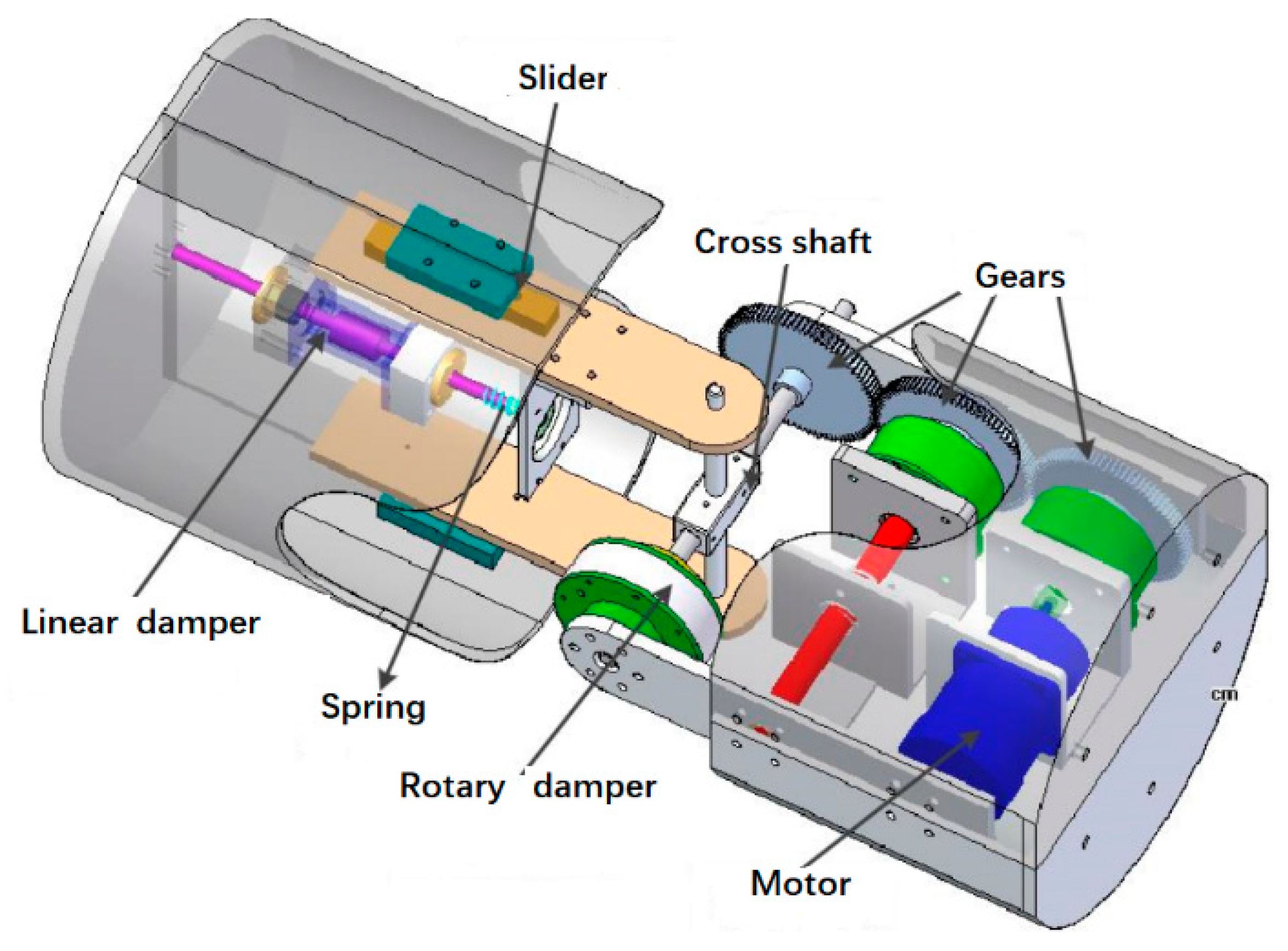
  • Buffer and unloading of spatial momentum: i.e., the decoupled dampers are necessary to be designed in the joint.
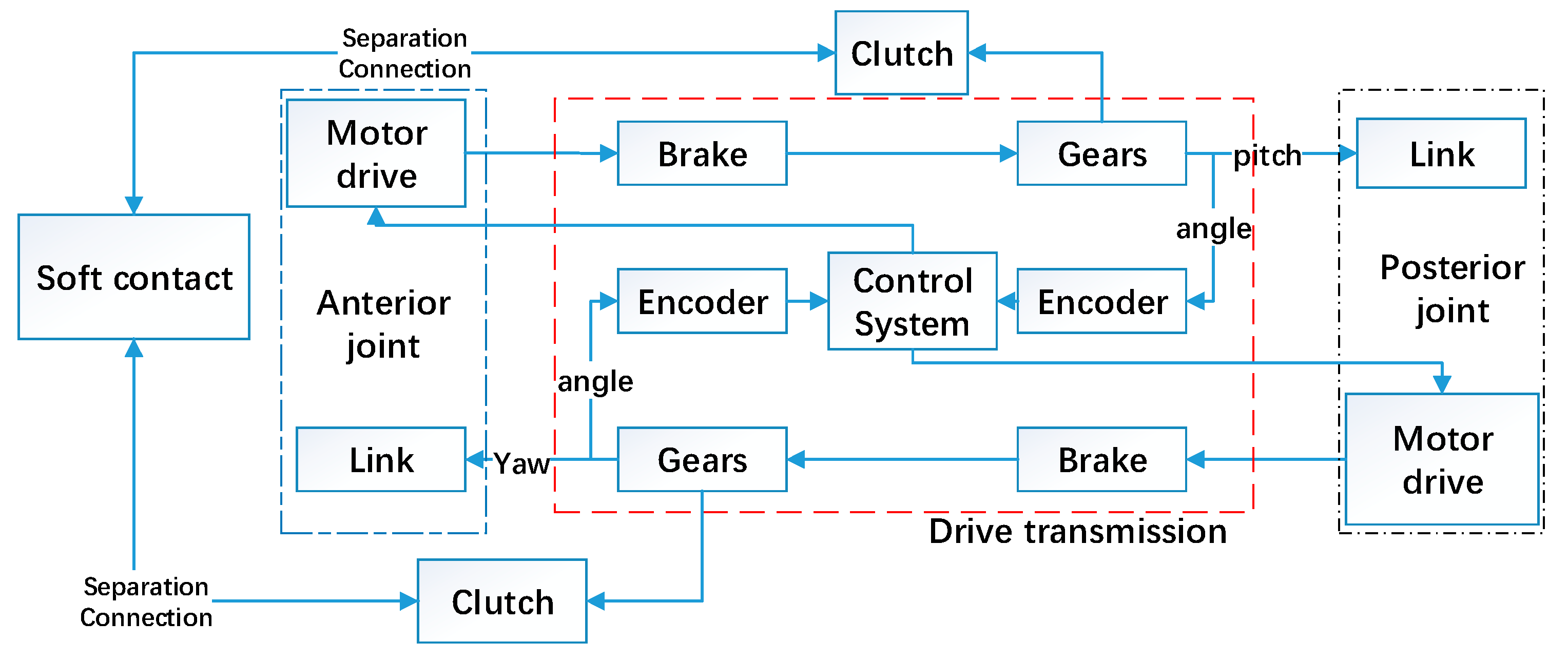
  • Dual modes switching: i.e., the motor transmission mode and soft contact mode can be controlled by clutch according to the on-orbit tasks.

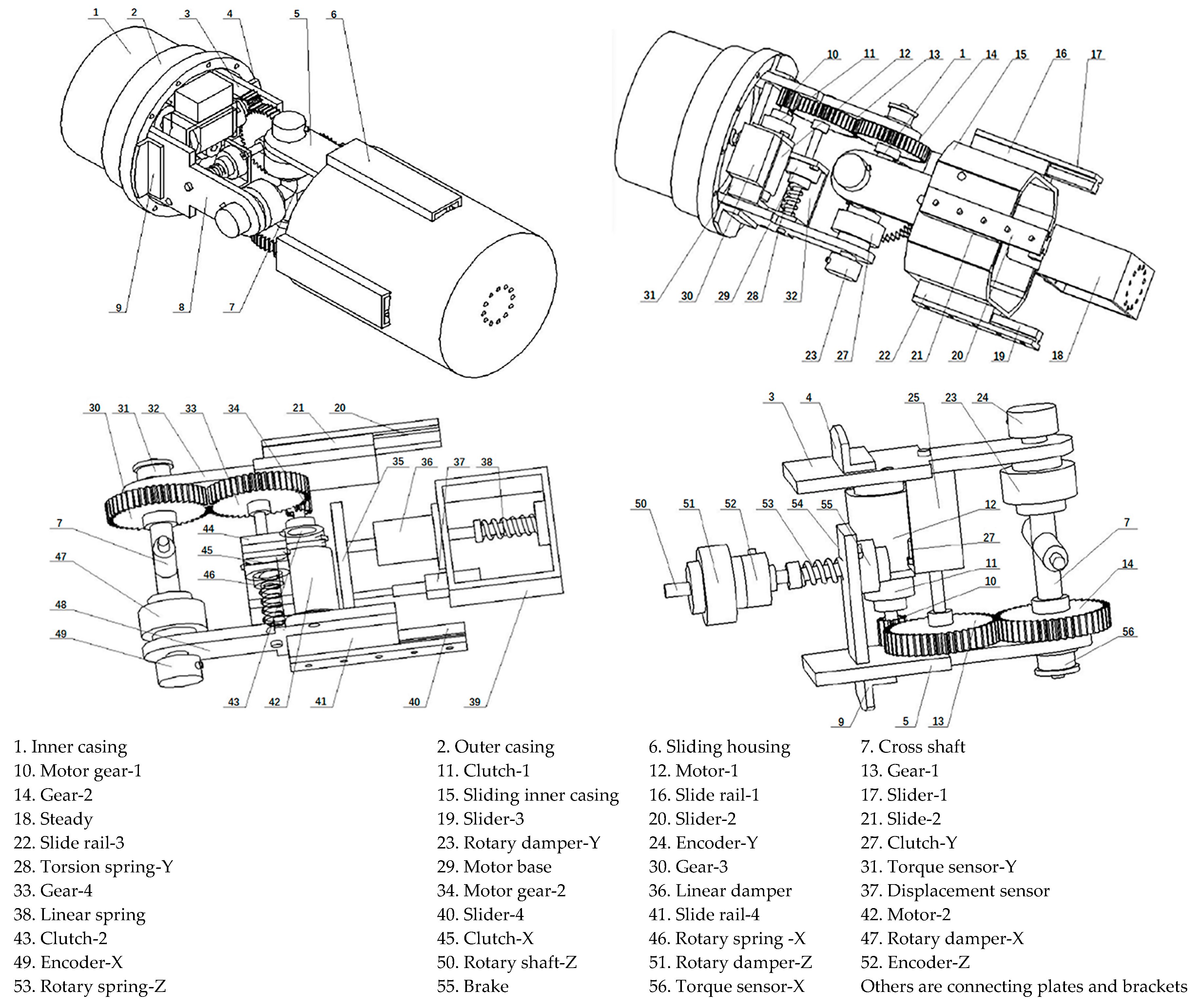
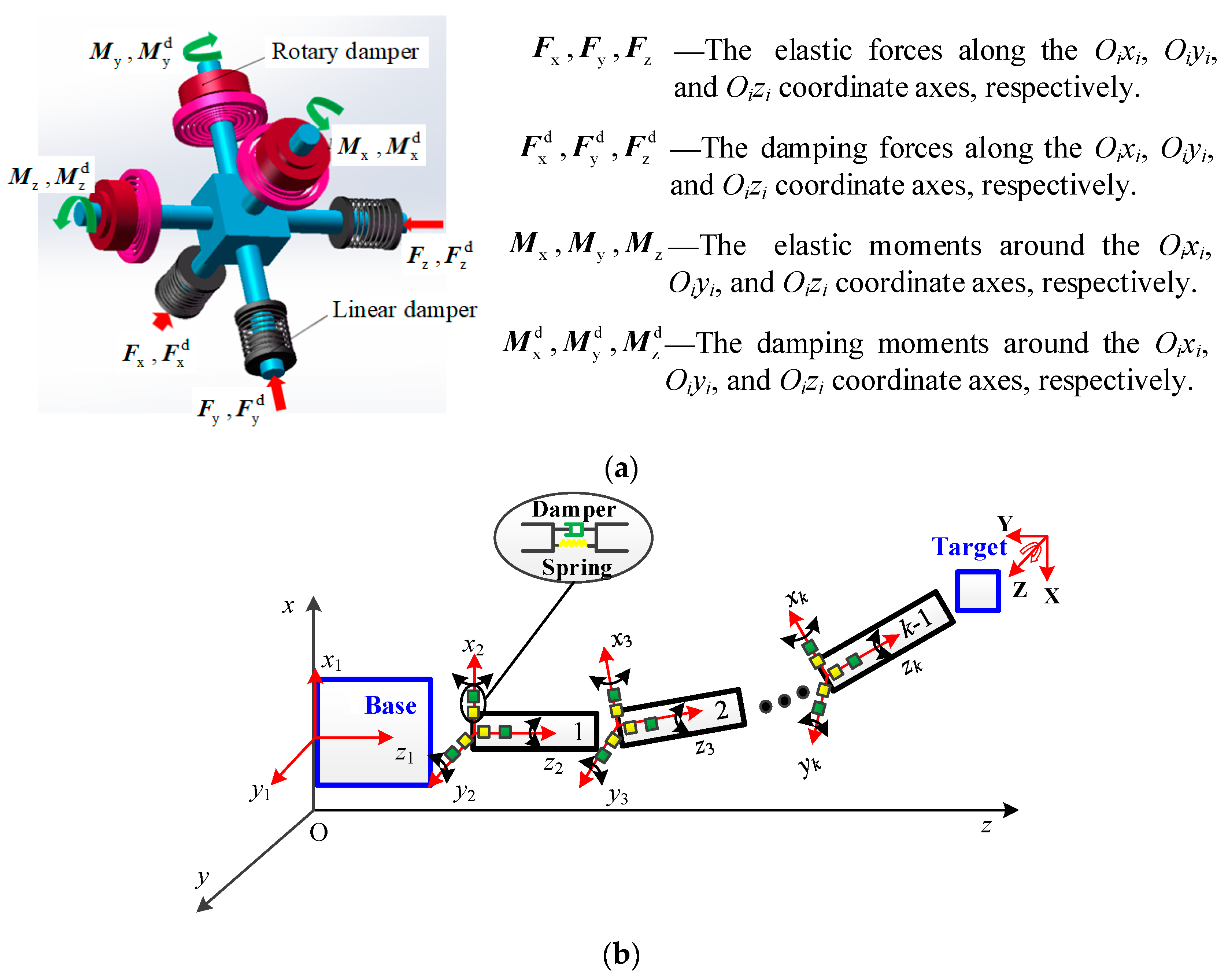
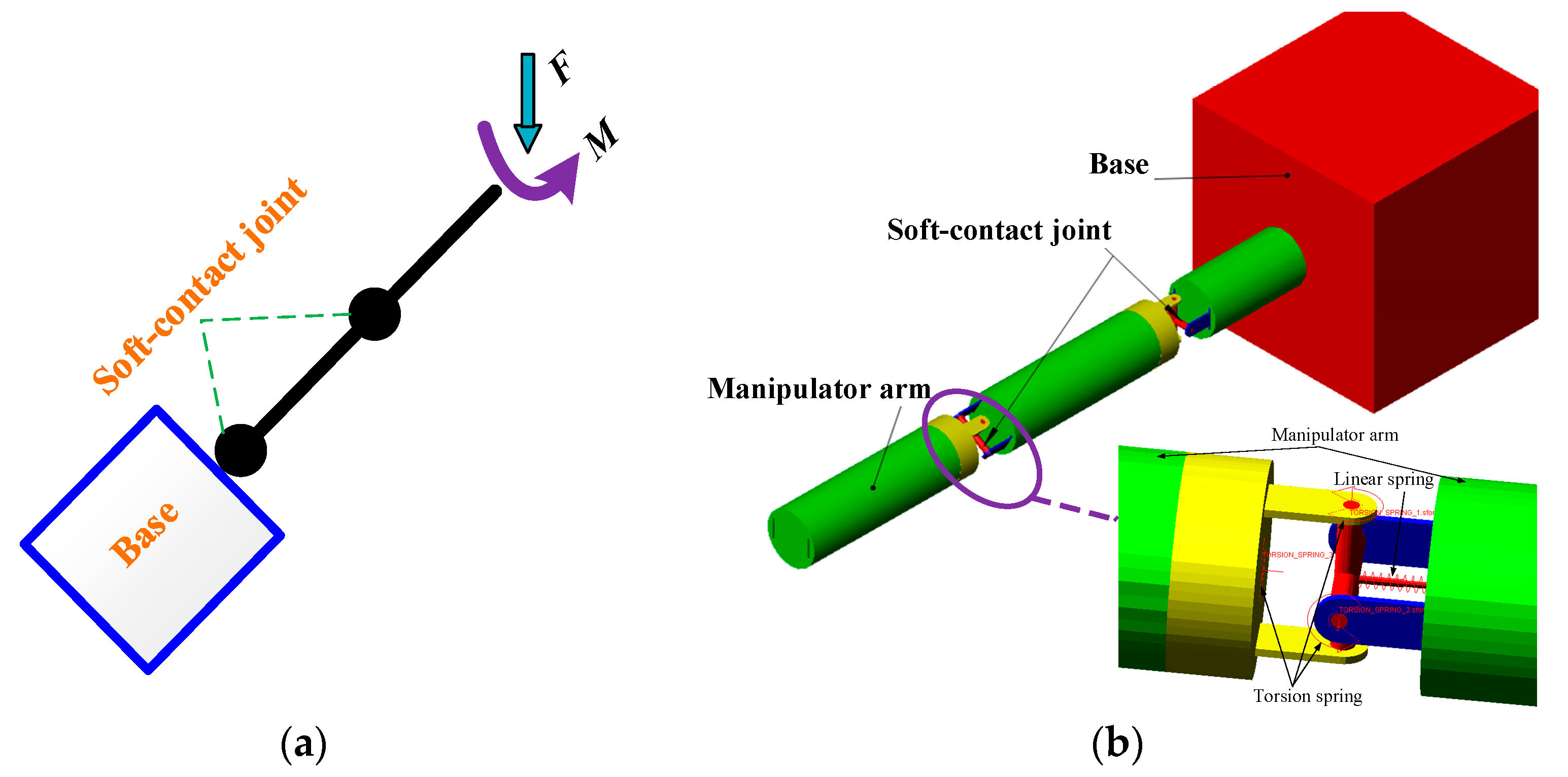
3. Structure Design of the Soft-contact Joint

To achieve the requirements of the above specific functions in Section 2, the joint-driving mechanism and decoupled dampers are separately designed. The soft-contact joint is 0.23 m in diameter and 0.75 m in length. Considering the size and structure of some key components, the cross-shaft structure can be adopted to realize orthogonal transmission by motors. The joint structure schemes are shown in Figure 2 and Figure 3. Linear spring/damper and rotary spring/damper are designed to buffer and unload the linear and rotational impact separately.
The block diagram of the dual working modes transmission is shown in Figure 4. The motors and gears are employed as the active driving to achieve the rotation movements of the cross shafts, and path planning for the manipulator could be performed. Additionally, the soft-capture operation could be realized by using the decoupled dampers through clutch switching.
The designed joint can work in dual modes. On the one hand, the spatial path-planning motion, especially for a manipulator connected by multi-joints and links, while each joint is driven by a two-DOF cross-shaft structure. On the other hand, utilizing the decoupled dampers, the joint can buffer the six-dimensional momentum introduced by spatial contact. The theoretical results of the former mode are very mature, so this article will not cover them but mainly show some contributions about the latter mode.
Considering the reasonable arrangement of the joint internal space, in the Cartesian coordinate system, it is necessary to design decoupled dampers only in the X/Y/Z-angle and Z-line directions of the joint; i.e., there are four DOFs totally to buffer and unload the impact. The dynamical principle block diagram is shown in Figure 5a. The momentum of the X/Y/Z-angle direction can be unloaded by the three rotary dampers and the linear momentum of the Z-line direction can be unloaded by the linear damper. In addition, Figure 5b shows the representative force (moment) diagram of two consecutive joints, and one can see that the axial force Fx(k+1) along the X-line direction can be converted into the rotational moments Myk around the Okyk axis and My(k-1) around the Ok-1yk-1 axis. Similarly, the axial force Fy(k+1) along the Y-line direction can be converted into the rotational moments Mxk around the Okxk axis and Mx(k-1) around the Ok-1xk-1 axis. Based on this principle, the collision linear momentum along the X-line direction and Y-line direction can be indirectly stabilized by rotating dampers existing in other joints.

4. Generalized Model of Manipulator

As shown in Figure 6a, Oixiyizi (i = 1, 2, 3, …, N + 1) is the ith joint’s coordinate system, where N is a natural number. Three linear dampers are respectively equipped along the Oixi, Oiyi, and Oizi coordinate axes. In addition, three rotary dampers are respectively equipped around the Oixi, Oiyi, and Oizi coordinate axes. One can see that linear damper and rotary damper can suppress impact and vibration in the linear and rotating directions, separately. As a result, the new-style joint with six-DOF can make the stabilization of impact momentum in the spatially six-dimensional directions.
If the N joints are connected in a series by the N links, a generalized model of manipulator with 6N-DOF multistage damping can be obtained. Figure 6b gives the sketch model, where Oxyz is the inertial coordinate system. Hence an N-joint manipulator with a free-floating base is equivalent to a base-fixed system with (6N + 6) DOFs. Using the Kane approach to model this series-wound system, the generalized differential equations are as follows.

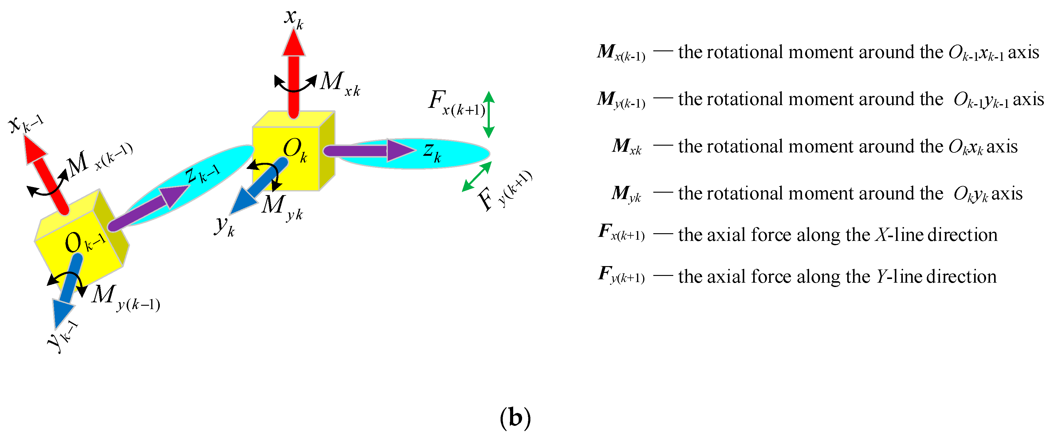
4.1. Transformation Matrix

As shown in Figure 6b, establish the inertial frame Oxyz and body-fixed coordinate system Okxkykzk (k = 1, 2, 3, …, N + 1) at the side of the kth segment. Due to the introduction of springs and dampers inside the joint, the manipulator evolves into a multi-flexible system with elastic deformation in six directions at each joint. In the dynamic equation, all deformation variables need to be solved, so it is difficult to describe these variables in a single coordinate system, but it can be easily expressed in each body-fixed coordinate system. At the same time, considering the huge number of variables and the pose transformation of each body-fixed coordinate system, it is not feasible to denote them with vectors, but the elements of each vector can be uniformly expressed. Define the relatively linear velocity v k k 1 and angular velocity ω k k 1 between the (k − 1)th and kth segments as the generalized velocity y l and relative displacement s k k 1 and angle θ k k 1 as generalized displacement x l , where the superscript (k − 1) and subscript k stand for the numbers of the body-fixed coordinate system about the (k − 1)th and kth segments separately.
y l = { ω k m k 1 l = 3 ( k 1 ) + m v k m k 1 l = 3 N + 3 + 3 ( k 1 ) + m x l = { θ k m k 1 l = 3 ( k 1 ) + m s k m k 1 l = 3 N + 3 + 3 ( k 1 ) + m
where m = 1, 2, and 3 corresponds to the three axes of x, y, and z in each body-fixed coordinate system, respectively.
The relative angles θ k 1 k 1 , θ k 2 k 1 , θ k 3 k 1 between the kth and (k − 1)th segments are adopted to describe the relative transformation matrix (Equation(2)) of O k x k y k z k relative to O k 1 x k 1 y k 1 z k 1 .
A k k 1 = Rot ( x , θ k 1 k 1 ) Rot ( y , θ k 2 k 1 ) Rot ( z , θ k 3 k 1 )
where Rot ( x , θ k 1 k 1 ) = ( 1 0 0 0 cos θ k 1 k 1 sin θ k 1 k 1 0 sin θ k 1 k 1 cos θ k 1 k 1 ) , Rot ( y , θ k 2 k 1 ) = ( cos θ k 2 k 1 0 sin θ k 2 k 1 0 1 0 sin θ k 2 k 1 0 cos θ k 2 k 1 ) , and Rot ( z , θ k 3 k 1 ) = ( cos θ k 3 k 1 sin θ k 3 k 1 0 sin θ k 3 k 1 cos θ k 3 k 1 0 0 0 1 ) .
The absolute transformation matrix of O k x k y k z k relative to the inertial system Oxyz is
A k R = A 0 R A 1 0 A 2 1 A k k 1
where A 0 R = E , an identity matrix, and the superscript “R” stands for the inertial frame Oxyz in Figure 6b.
As can be seen from Equation (2), in the process of theoretical modeling, we assume that the manipulator is firstly rotated by θ k 1 k 1 around the X-axis of the generalized coordinate system O k 1 x k 1 y k 1 z k 1 , then rotated by θ k 2 k 1 around the Y-axis of the generalized coordinate, and finally, rotated by θ k 3 k 1 to the Z-axis of the generalized coordinate. The generalized angular velocity is defined in the initially generalized coordinate O k 1 x k 1 y k 1 z k 1 , so the relationship between the generalized angular velocity ω k k 1 and the derivative of the generalized angular displacement θ k 1 k 1 , θ k 2 k 1 , θ k 3 k 1 is as follows:
( ω k 1 k 1 ω k 2 k 1 ω k 3 k 1 ) = ( θ ˙ k 1 k 1 0 0 ) + Rot ( x , θ k 1 k 1 ) ( 0 θ ˙ k 2 k 1 0 ) + Rot ( x , θ k 1 k 1 ) Rot ( y , θ k 2 k 1 ) ( 0 0 θ ˙ k 3 k 1 )
Hence, the kinematics equation can be derived and expressed as follows:
( θ ˙ k 1 k 1 θ ˙ k 2 k 1 θ ˙ k 3 k 1 ) = 1 cos θ k 2 k 1 ( cos θ k 2 k 1 sin θ k 1 k 1 sin θ k 2 k 1 cos θ k 1 k 1 sin θ k 2 k 1 0 cos θ k 1 k 1 cos θ k 2 k 1 sin θ k 1 k 1 cos θ k 2 k 1 0 sin θ k 1 k 1 cos θ k 1 k 1 ) ( ω k 1 k 1 ω k 2 k 1 ω k 3 k 1 )
( v k 1 k 1 v k 2 k 1 v k 3 k 1 ) = d d t ( s k 1 k 1 s k 2 k 1 s k 3 k 1 )

4.2. Partial Angular Velocity and Partial Linear Velocity

Angular velocity of the kth segment in the inertial frame can be expressed as:
ω k R = A 0 R ω 1 0 + A 1 R ω 2 1 + + A k 1 R ω k k 1 = i = 1 k A i 1 R ω i i 1
According to the definition of partial angular velocity,
[ ω k l ] 3 × 1 = { ω k R ω i m i 1 l = 3 ( i 1 ) + m ω k R v i m i 1 l = 3 N + 3 ( i 1 ) + m
Substitute Equation (7) into Equation (8) to derive the partial angular velocity, and a total matrix can be used to save the partial angular velocity of the kth segment relative to y l .
[ W k l ] 3 × ( 6 N + 6 ) = ( A 0 R A 1 R A k 1 R 0 )
where l = 1, 2, 3, …, 6N + 6.
Position vector of the centroid of the kth segment in the inertial frame can be formulated by
p k R = p RO + A 0 R s 1 0 + i = 1 k 1 A i R ( d i + s i + 1 i ) + A k R r k
where:
  • p RO —position vector of O1x1y1z1 in the inertial frame,
  • d i —position vector of the ith segment in Oixiyizi, and
  • r k —vector of the centroid of the kth segment in Okxkykzk.
Taking the derivative of Equation (10) with respect to time, the velocity of the centroid of the kth segment in the inertial system is derived as follows:
v k R = A 0 R s ˙ 1 0 + i = 1 k 1 [ A ˙ i R ( d i + s i + 1 i ) + A ˙ i R s ˙ i + 1 i ] + A ˙ k R r k
According to the definition of partial velocity,
[ v k l ] 3 × 1 = { v k R ω i m i 1 l = 3 ( i 1 ) + m v k R v i m i 1 l = 3 N + 3 ( i 1 ) + m
where i = 1, 2, 3, …, N + 1. Substituting Equation (11) into Equation (12), the partial velocity of the kth segment relative to y l is as follows:
[ v k l ] 3 × 1 = { i = 1 k 1 ω i l × A i R ( d i + s i + 1 i ) + ω k l × A k R r k ( l 3 k ) 0 ( 3 k l 3 N + 3 ) ω k ( l 3 N 3 )   ( 3 N + 3 l 3 N + 3 k + 3 ) 0 ( 3 N + 3 k + 3 l 6 N + 6 )

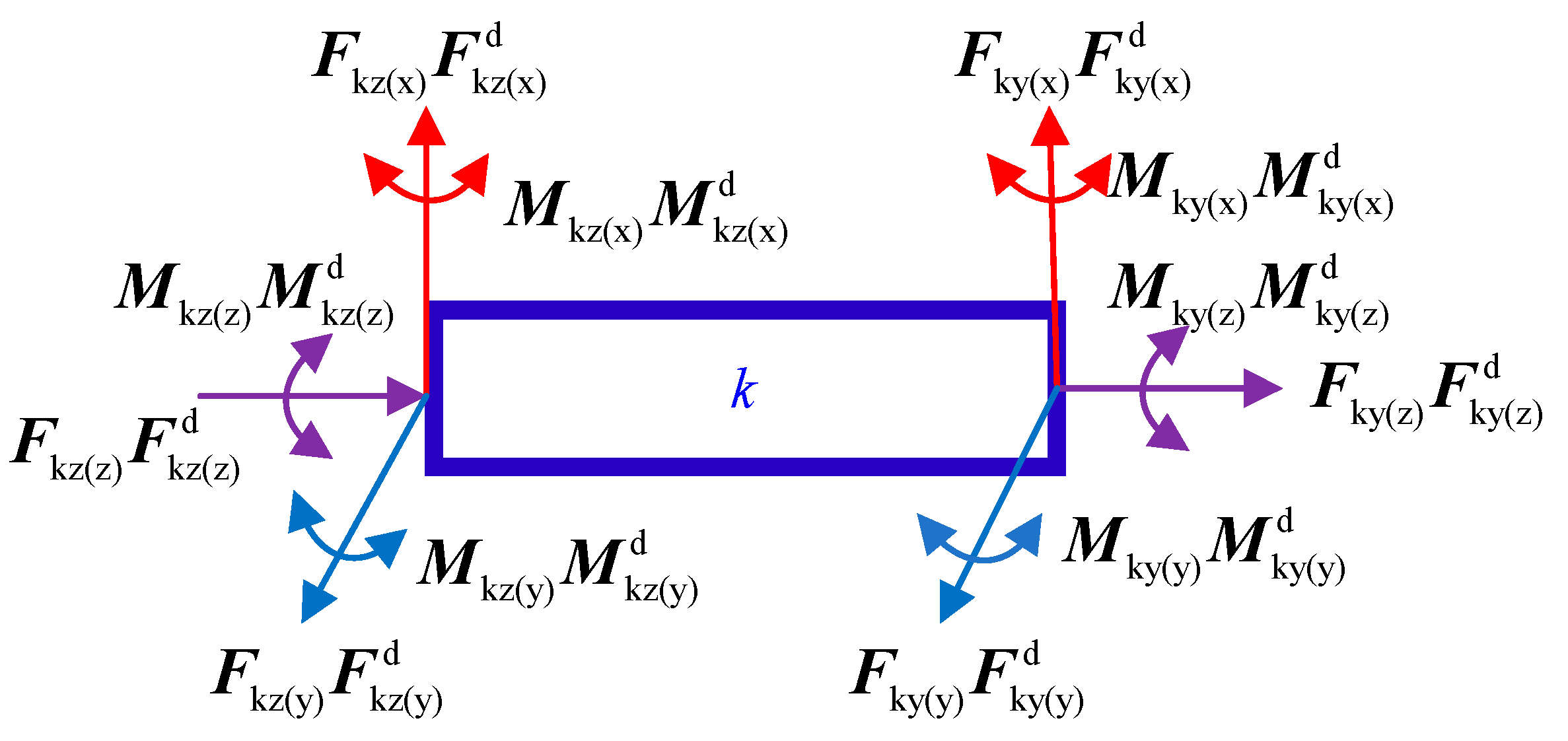
4.3. Equivalent Active Force and Equivalent Inertia Force

Figure 7 shows the stress analysis for the kth segment. The active forces in the left side are elastic deformation forces (i.e., F k z and M k z ) and damping forces (i.e., F k z d and M k z d ) of decoupled dampers in six directions. While, in the right side, the active forces are elastic deformation forces (i.e., F k y and M k y ) and damping forces (i.e., F k y d and M k y d ). Gravity can be ignored due to the tiny centripetal acceleration in the space environment.
According to the transforming matrix, the elastic deformation forces in both sides of the kth segment are as follows:
( F k z , M k z , F k y , M k y ) R T = diag ( A k R , A k R , A k R , A k R ) diag ( K 1 , K 2 , K 3 , K 4 ) diag ( A k 1 k , A k 1 k , E , E ) ( s k k 1 , θ k k 1 , s k + 1 k , s k + 1 k ) T
where:
  • Fkz—the elastic force on the left side,
  • Mkz—the elastic torque on the left side,
  • Fky—the elastic force on the right side,
  • Mky—the elastic torque on the right side,
  • K1—the elastic coefficient matrix of the left linear damper,
  • K2—the elastic coefficient matrix of the left rotary damper,
  • K3—the elastic coefficient matrix of the right linear damper, and
  • K4—the elastic coefficient matrix of the right rotary damper.
The equivalent active force Fkc and active torque Mkc of each centroid can be described as:
(i) The base (k = 1, means the 1st segment).
There is no joint on the left side of the free-floating base, and only the right side is affected by joint 1. Expression is as follows:
{ F 1 c = F 1 y M 1 c = M 1 y + A 1 R r 1 × F 1 y
(ii) The middle segments (1 < k < N + 1).
{ F k c = F k z + F u k z + F k y M k c = M k z + M u k z + M k y + A k R × r k × ( F k z F k z d + F k y )
where Fkz = −F(k-1)y, Mkz = −M(k-1)y.
(iii). The last segment (k = N + 1).
{ F ( N + 1 ) c = F ( N + 1 ) z + F ( N + 1 ) z d + F M ( N + 1 ) c = M ( N + 1 ) z + M ( N + 1 ) z d + M + A ( N + 1 ) R × r ( N + 1 ) × ( F ( N + 1 ) z + F ( N + 1 ) z d + F )
where
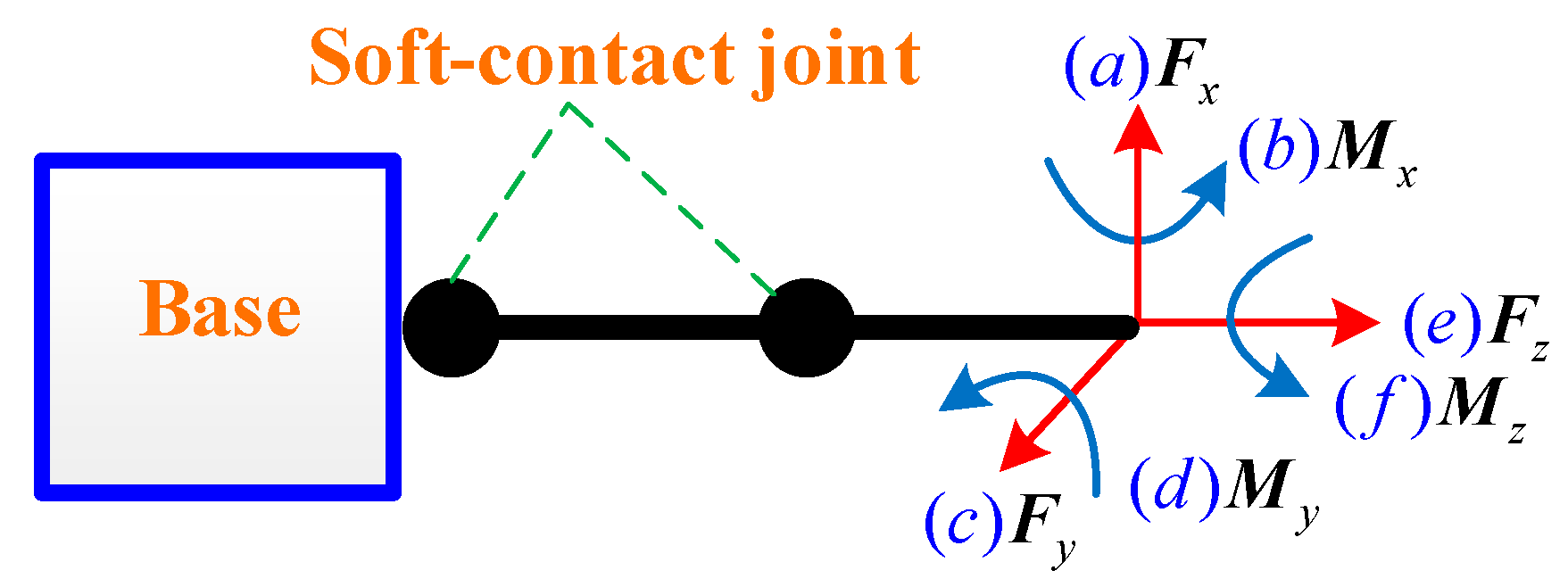
  • F—instantaneous impact force at the end of manipulator, and
  • M—instantaneous impact torque at the end of manipulator.
Next, the equivalent inertia force F k c and the equivalent inertia torque M k c of the kth segment are derived:
{ F k c = m k a k c M k c = I k ω ˙ k ω k × ( I k ω k )
where
  • mk—mass of the kth segment,
    Ik—inertia tensor of the kth segment,
  • ω ˙ k —angular acceleration of the kth segment,
  • akc—acceleration of the centroid of the kth segment, and
  • ωk—angular velocity of the kth segment.

4.4. Dynamic Equations

For a tandem mechanism with the (N + 1) segments, the Kane dynamic equations can be written as:
F l + F l = k = 1 N + 1 ( F k c v k l + M k c ω k l ) + k = 1 N + 1 ( F k c v k l + M k c ω k l ) = 0
where l = 1, 2, 3, …, 6N + 6.
Substituting the partial angular velocity, partial linear velocity, equivalent active force (torque), and equivalent inertia force (torque) into Equation (19) and combining dynamic Equation (5), the (6N + 6) dimensional nonlinear differential equations of the manipulator with multistage damping can be expressed as:
[ y ˙ η ] ( 6 N + 6 ) × 1 = [ a l η ] ( 6 N + 6 ) × ( 6 N + 6 ) 1 [ f l ] ( 6 N + 6 ) × 1
where
  • η = 1, 2, 3, …, 6N + 6;
  • f l = F l η = 1 6 N + 6 ( k = 1 N + 1 v k l T m k v ˙ k η + k = 1 N + 1 ω k l T I k ω ˙ k η ) y η k = 1 N + 1 ω k l T [ ω k R × ( I k ω k R ) ]
  • a l η = k = 1 N + 1 v k l T m k v k η + k = 1 N ω k l T I k ω k η

5. Instance Simulation

In this section, as shown in Figure 8a, a floating-base equipped with a two-joint manipulator, which has eight DOFs for compliance, is studied employing both MATLAB and Adams software. It is noteworthy that the derivational dynamic Equations (20) established in Section 4 play an important part in the fast numerical simulation in MATLAB, and therefore, the comparison with the Adams simulation results could be helpful for the effectiveness of Equations (20). Two kinds of typical target collisions are purposefully designed, namely, single-dimensional collision and spatially six-dimensional collision. The former simulation is mainly to prove that the designed soft-contact joint has the ability to buffer and unload the collision force from any spatial direction. The latter simulation is mainly to verify that multiple tandem joints have the obvious adaptability to protect the base from spatial impact.
In the Adams environment, as shown in Figure 8b, the two-joint floating base/manipulator with eight-DOF consists of two soft-contact joints, each of which has three DOFs of rotation and one linear DOF along the central axis of the link. The Z-line stiffness and damping values of the joints are set by the linear springs, the X-angle, Y-angle, and Z-angle stiffness, and the damping values of the joints are set by rotary springs. The cross shafts can move back and forth along the central axis of the link.

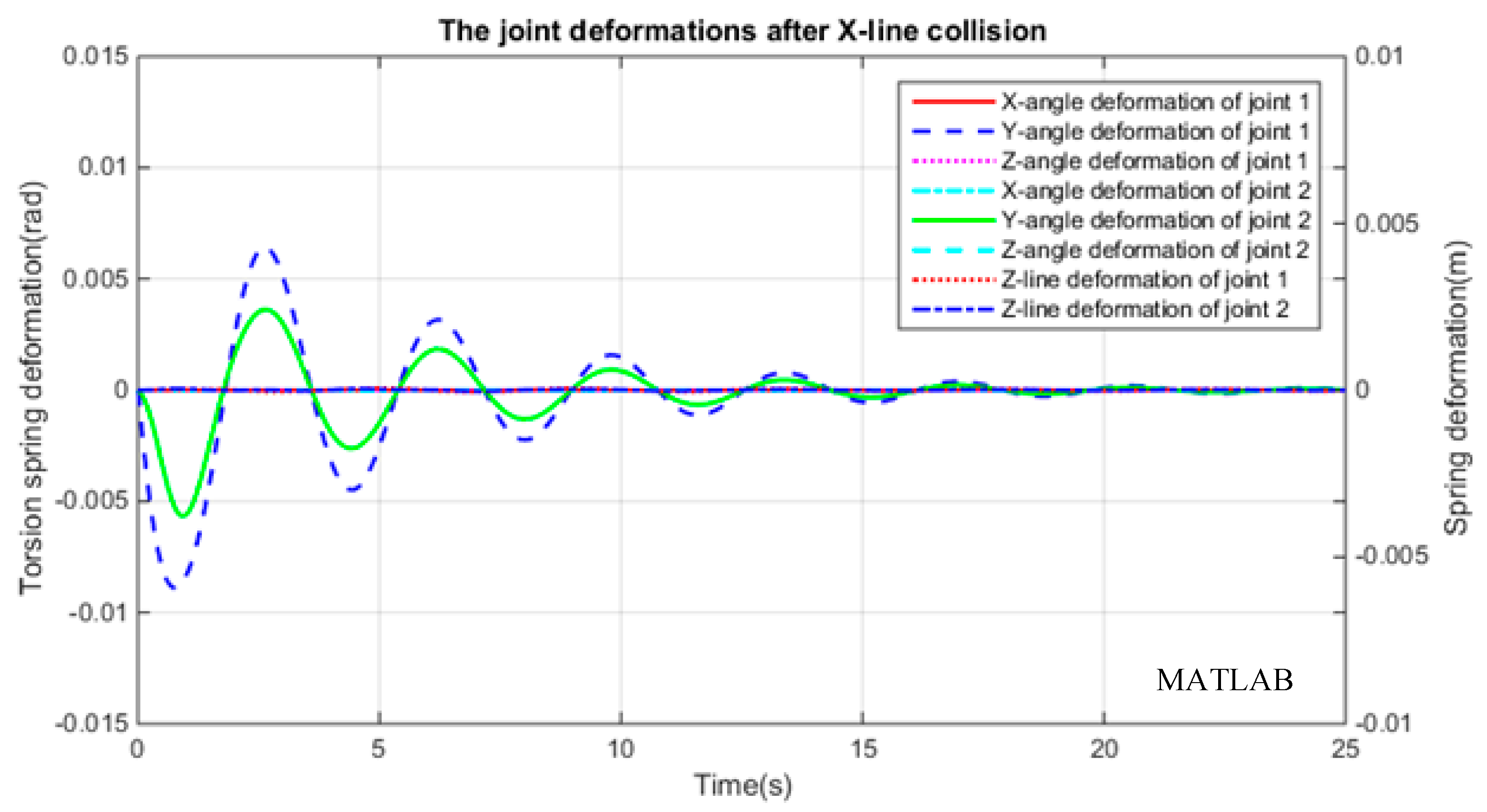
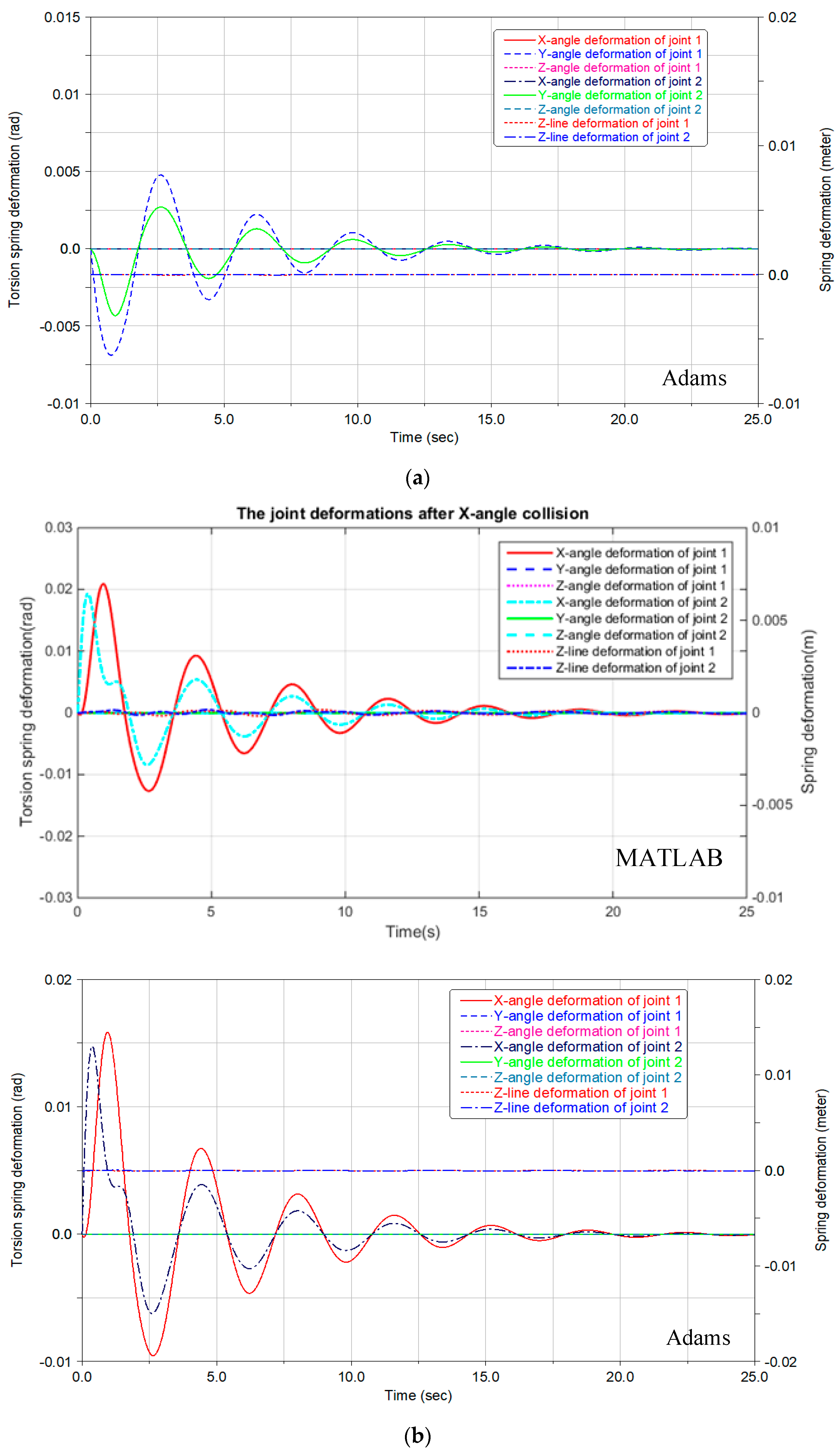
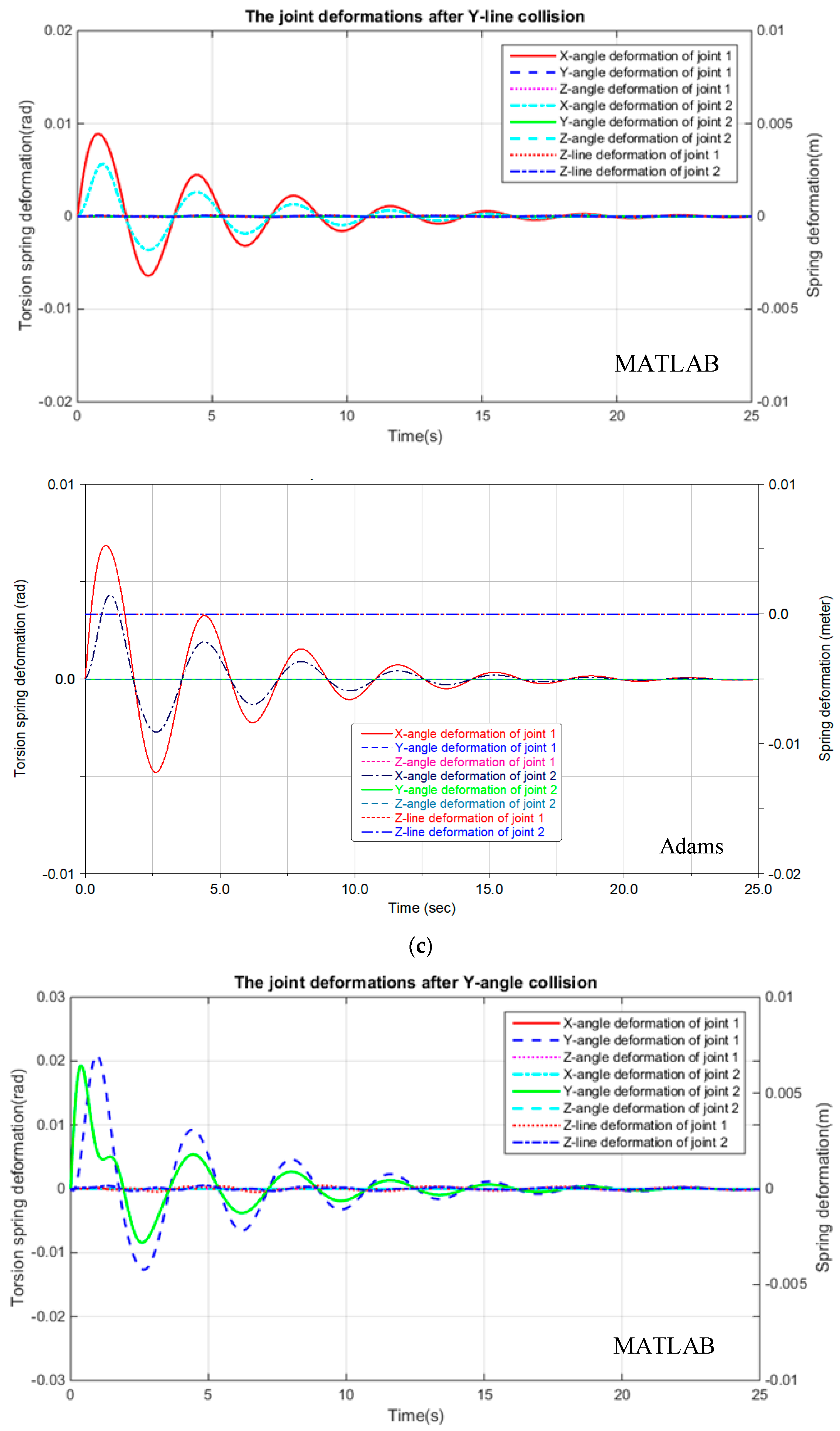
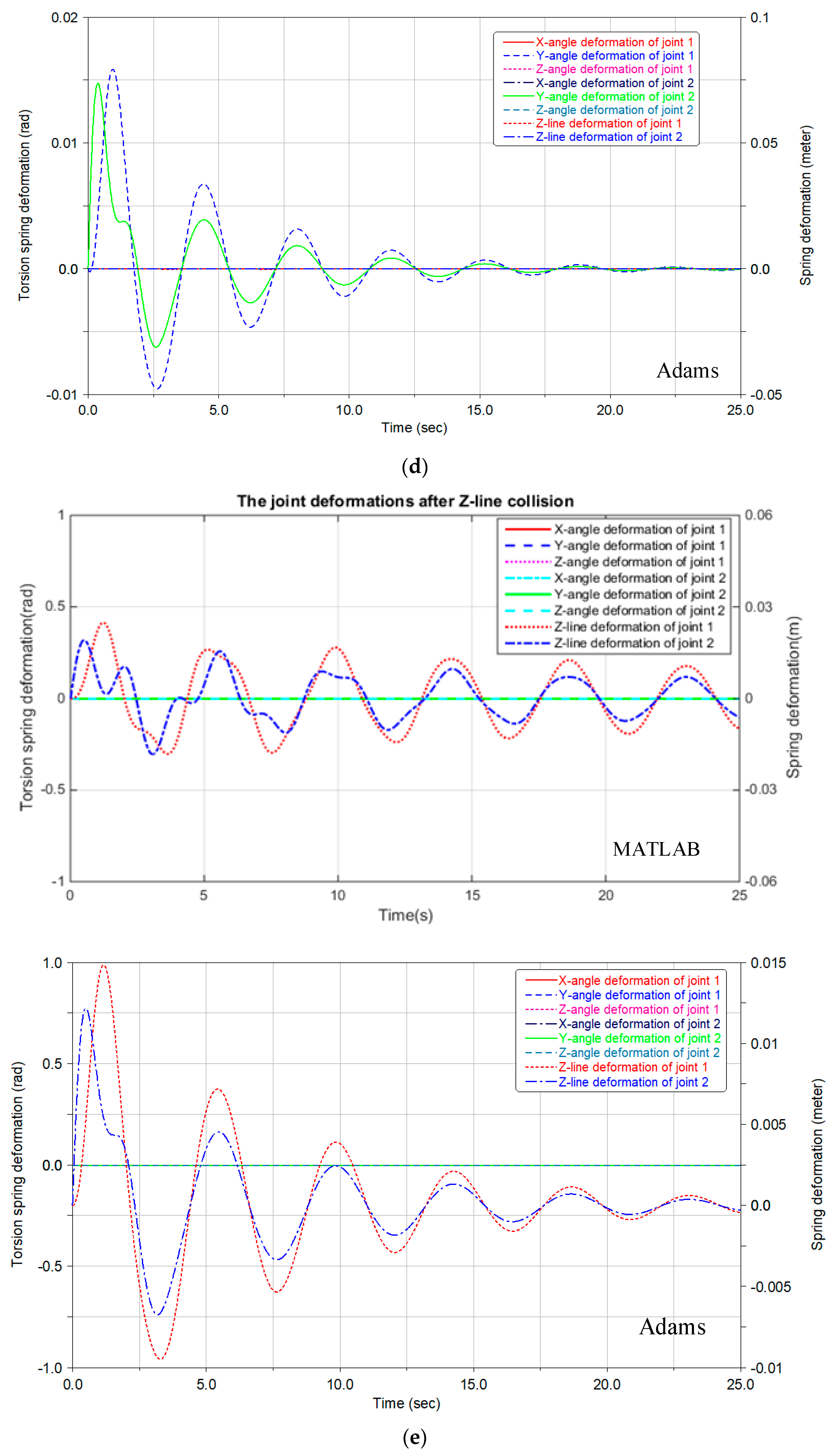
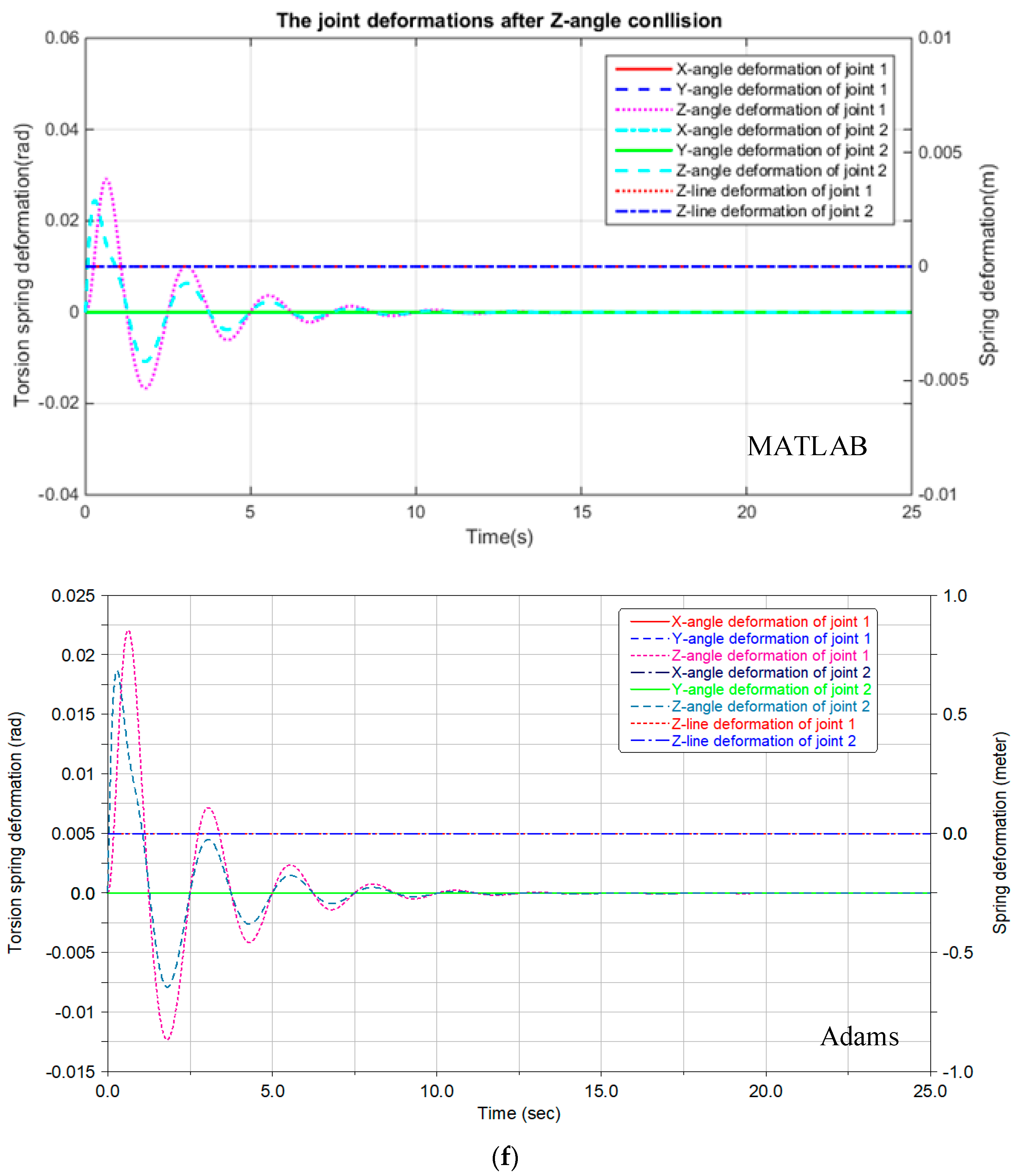
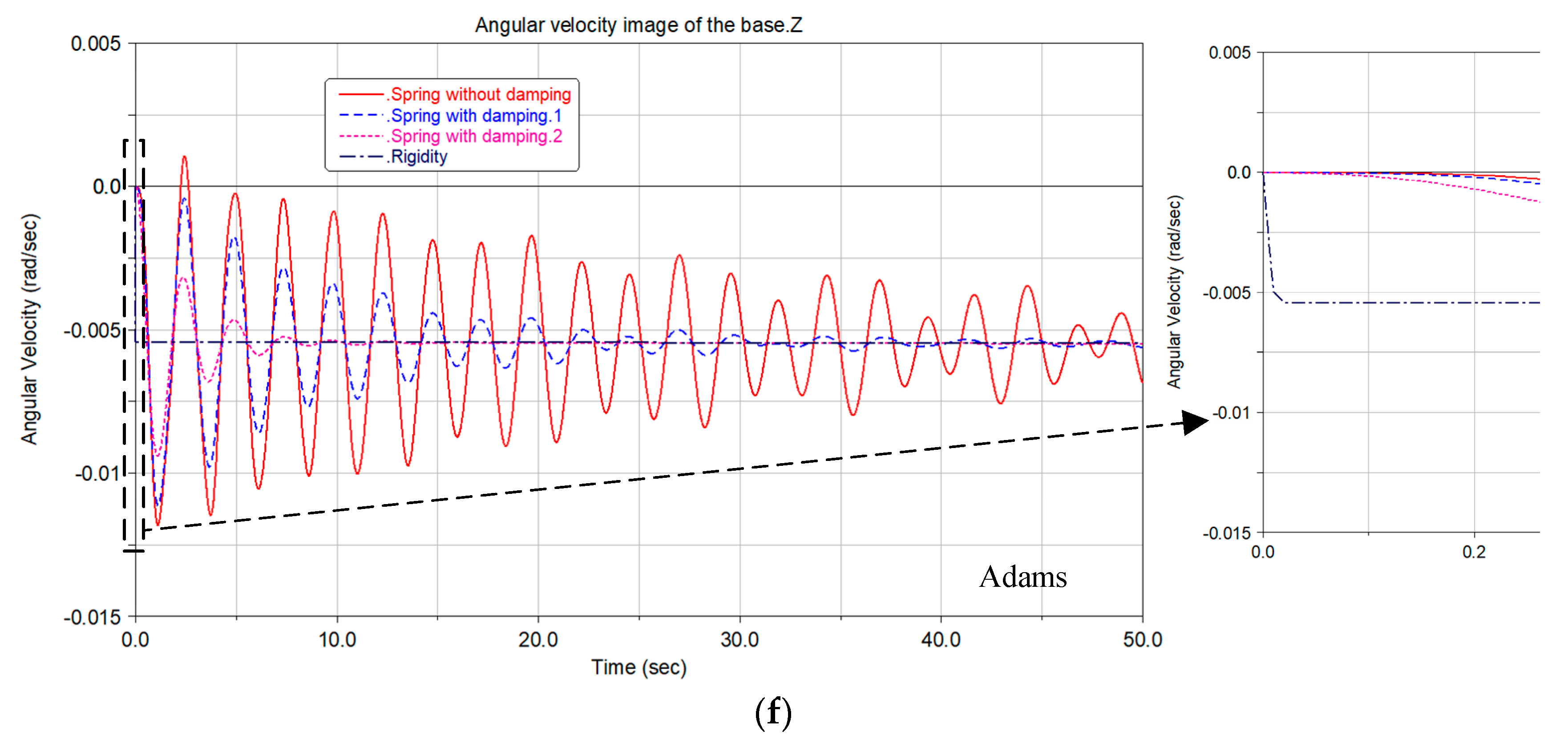
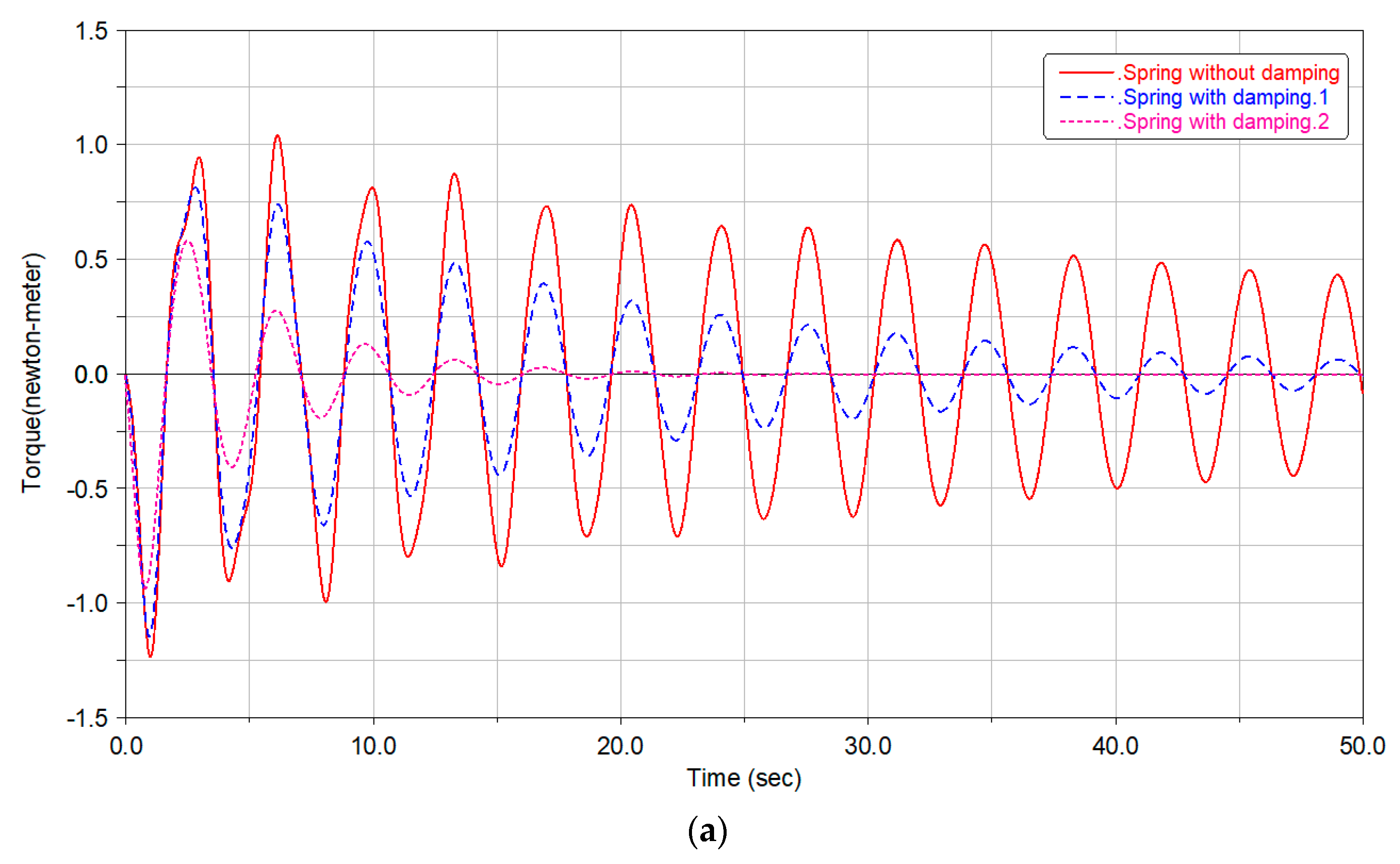
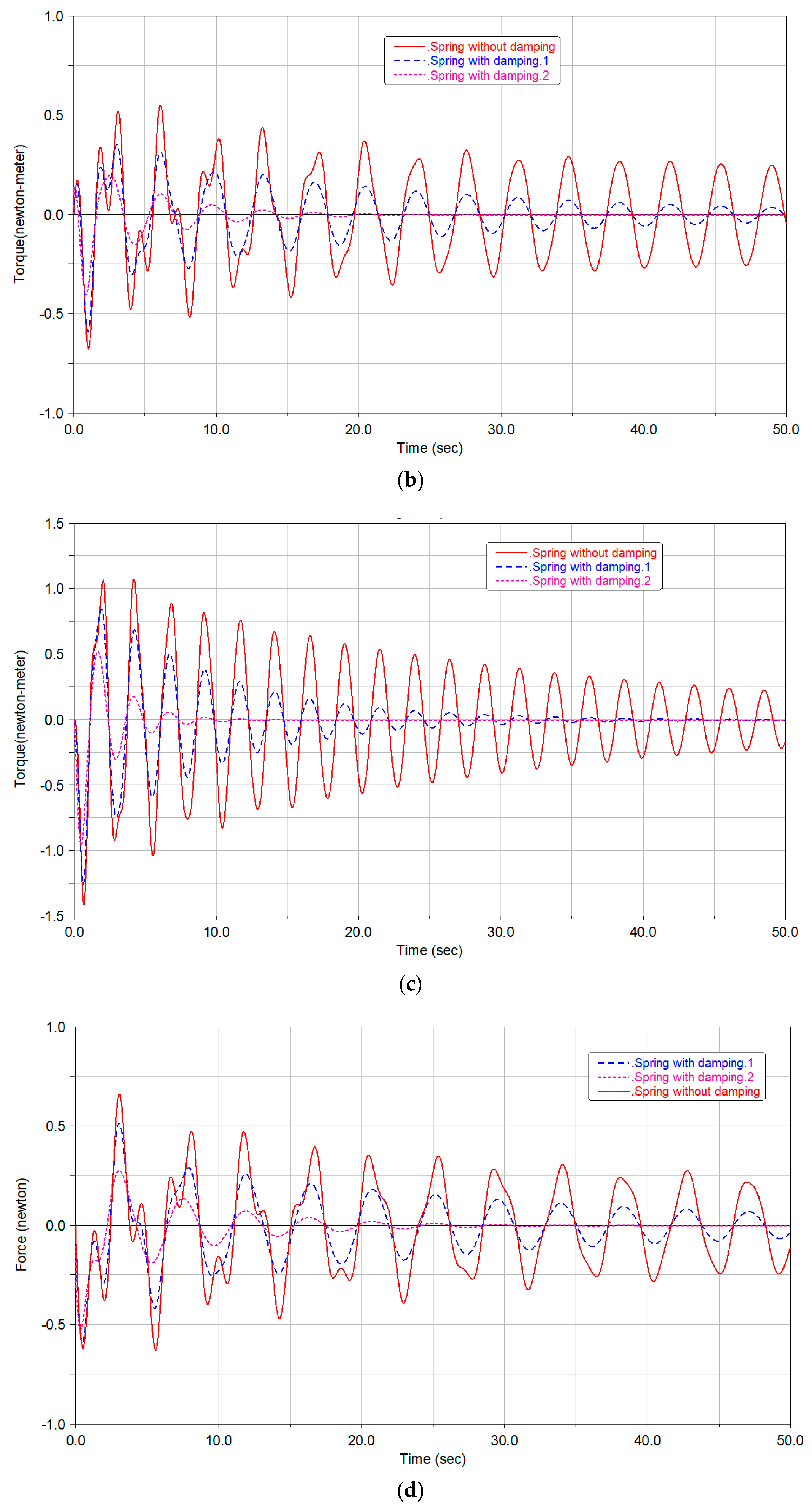
5.1. Single-Dimensional Collision

The developed soft-contact joint is expected to have the capability of both buffering and unloading momentum in any direction. In this section, as shown in Figure 9, six unidirectional collision forces, i.e., (a) Fx, namely, the X-line force, (b) Mx, namely, the X-angle moment, (c) Fy, namely, the Y-line force, (d) My, namely, the Y-angle moment, (e) Fz, namely, the Z-line force, and (f) Mz, namely, the Z-angle moment, are sequentially applied at the end of the space-borne manipulator, respectively. The unloading and buffering effects can be judged by measuring the spring deformations in the joints.
Specific simulation parameters are as follows. The values of the single-direction force or torque existing at the end of manipulator are 50 N or 50 N·m, and the duration is 0.01 s. Mass of base is 200 kg. Inertia moments of the base are Ix = Iy = 53.3 kg m 2 and Iz = 66.7 kg m 2 . Mass of each segment is 8 kg. Inertia moments of each segment are Ix = Iy = 5 kg m 2 and Iz = 2.5 kg m 2 . Elastic coefficients of the damper are fwx = fwy = fwz = 40 N m rad 1 and fz = 40 N m 1 , and each damping coefficient is 1.0 N·s·m−1 or 5.0 N·s·rad−1. The simulation step is 0.01 second.
As shown in Figure 10, the MATLAB and Adams simulation results are comparatively carried out. The vibration displacements of each compliance DOF in every joint under the single-dimensional collision are given respectively. It can be seen that, when the end of the manipulator is only subjected to X-line or Y-angle collision, only Y-angle deformations of the joints are produced, and when the end of the manipulator is only subjected to Y-line or X-angle collision, only X-angle deformations of the joints are produced. When the end of the manipulator is only subjected to the Z-angle collision, only Z-angle deformations of the joints are produced, and when the end of the manipulator is only subjected to a single Z-line collision, only Z-line deformations of the joints are produced. Moreover, all joint movements can converge under the action of damping, and the soft-contact principle proposed in Figure 5 can be verified.

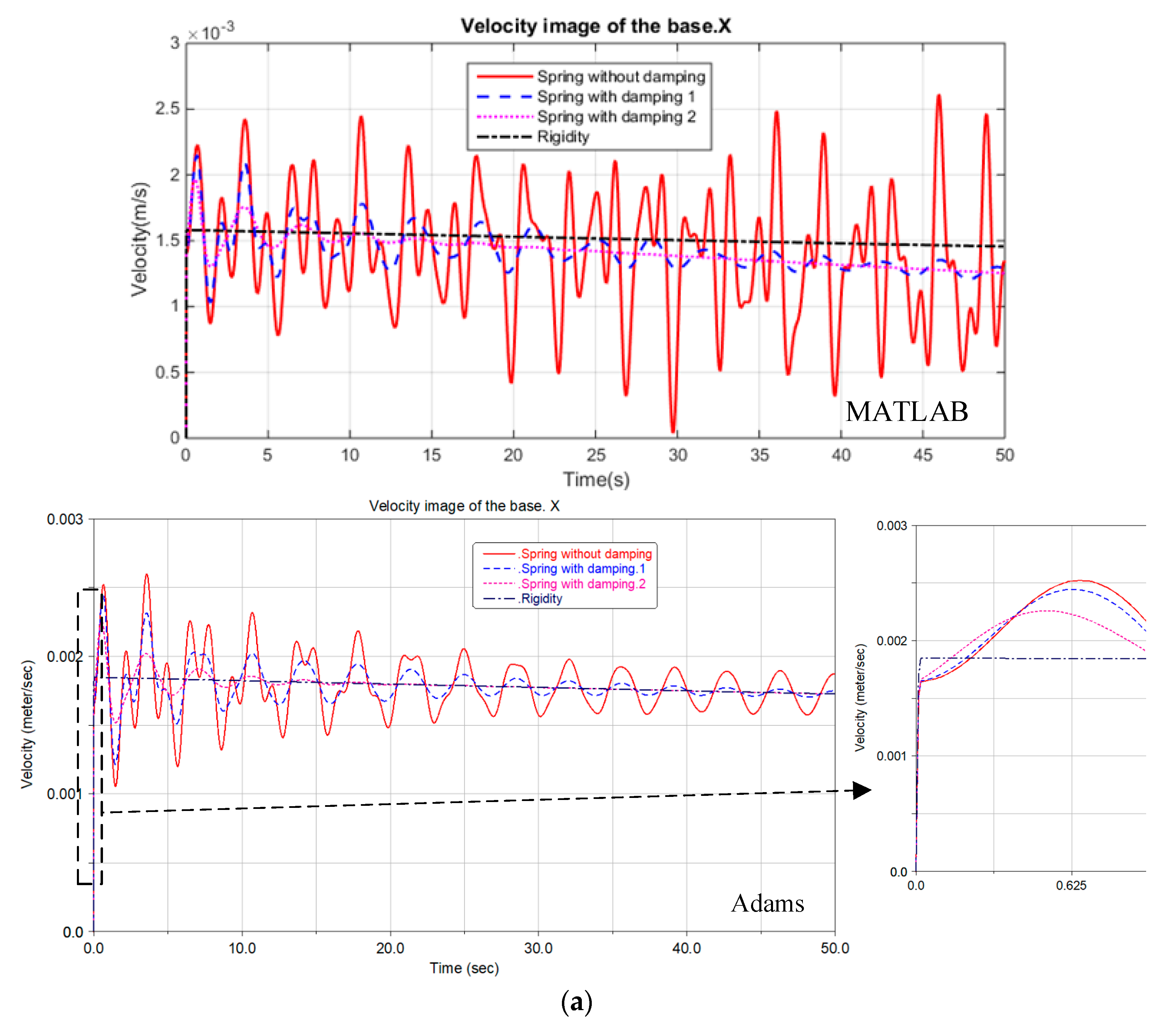
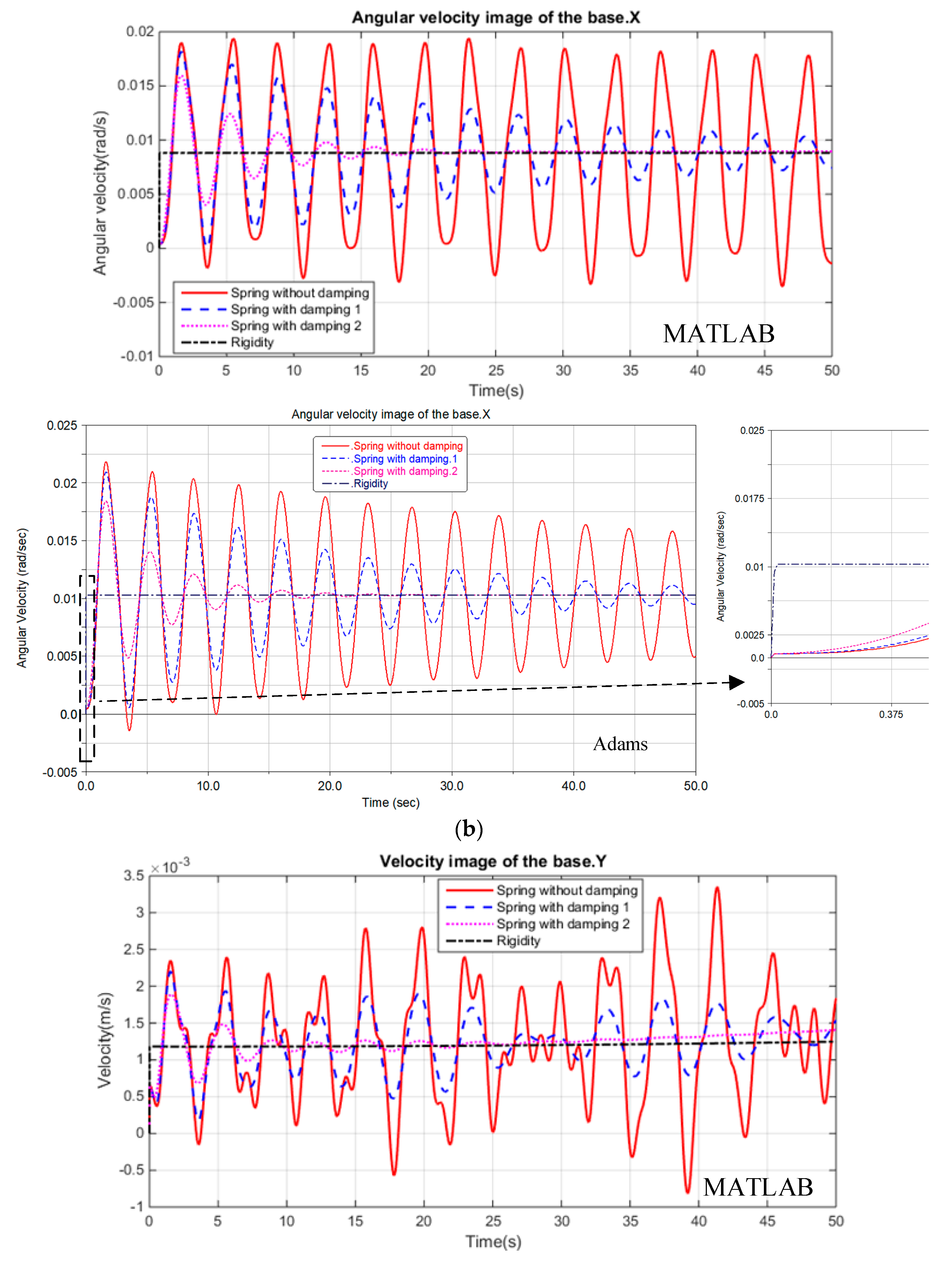
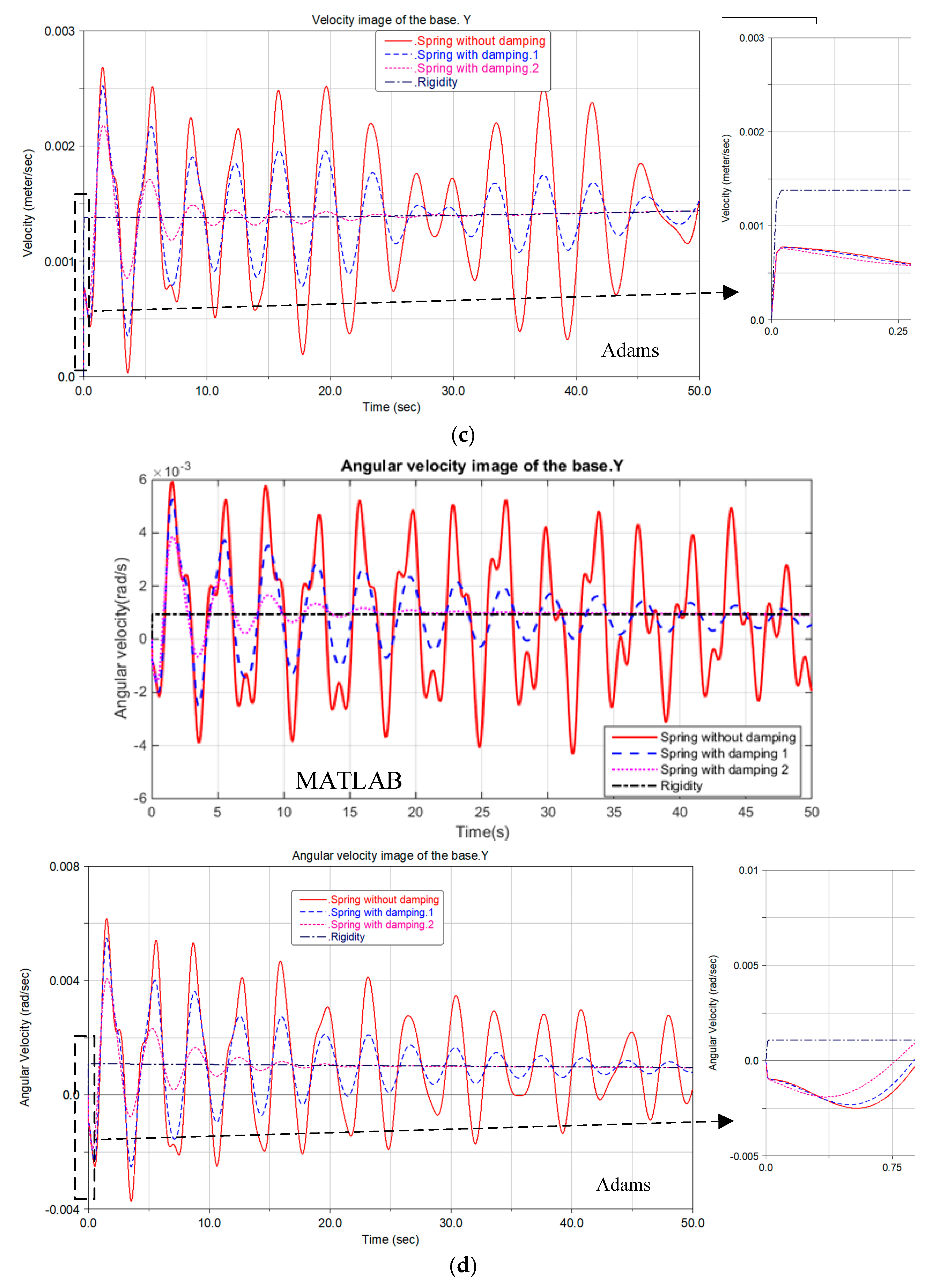
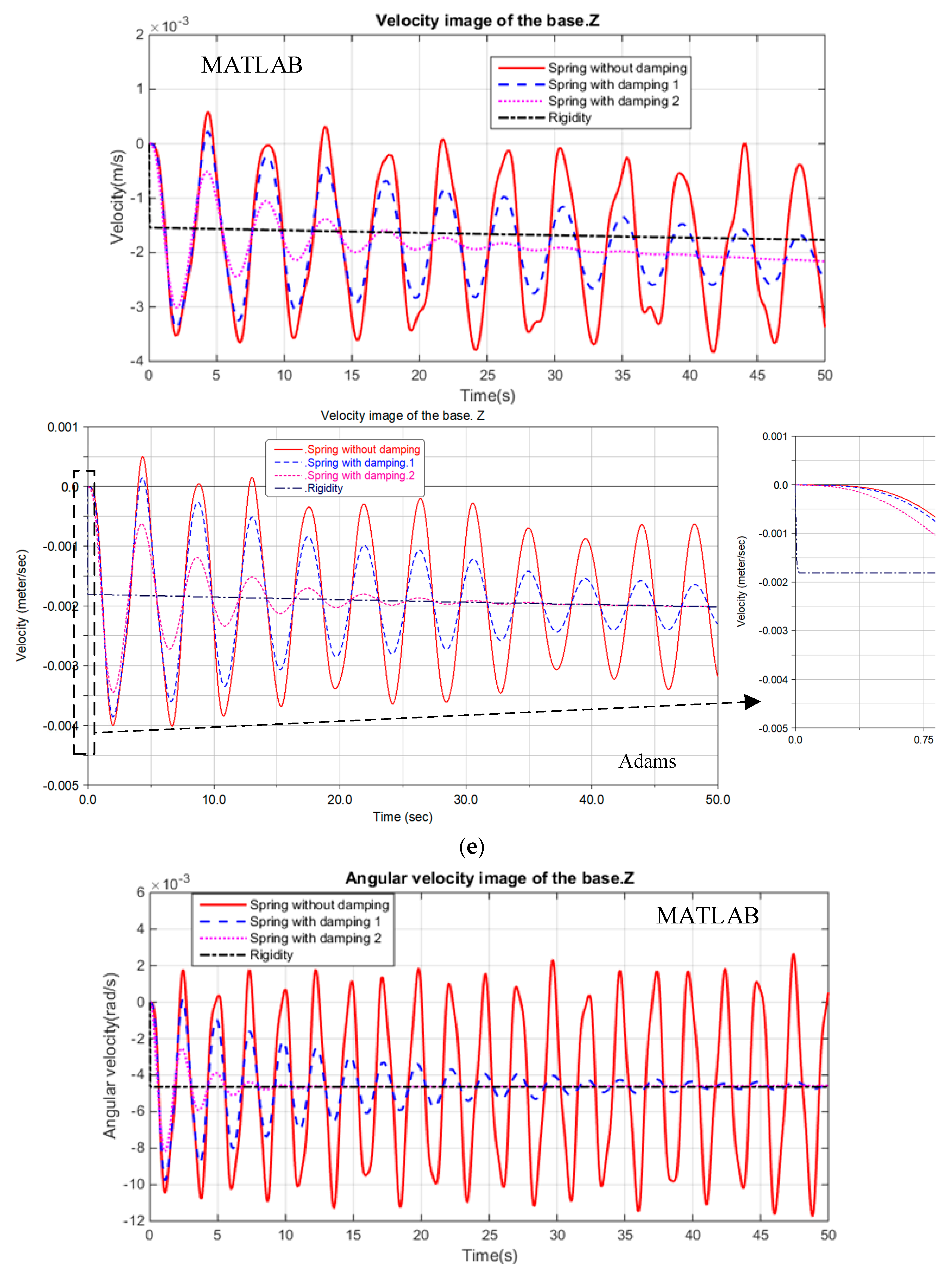
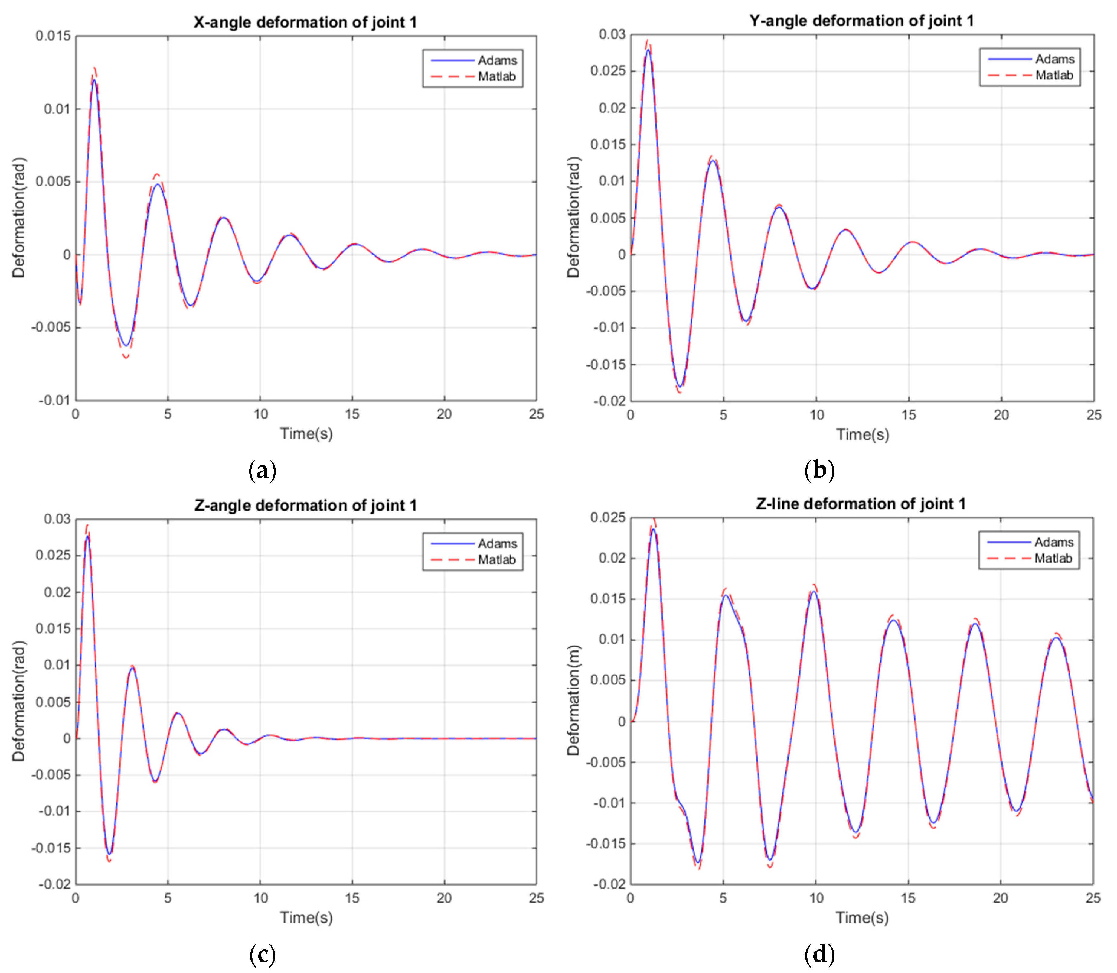
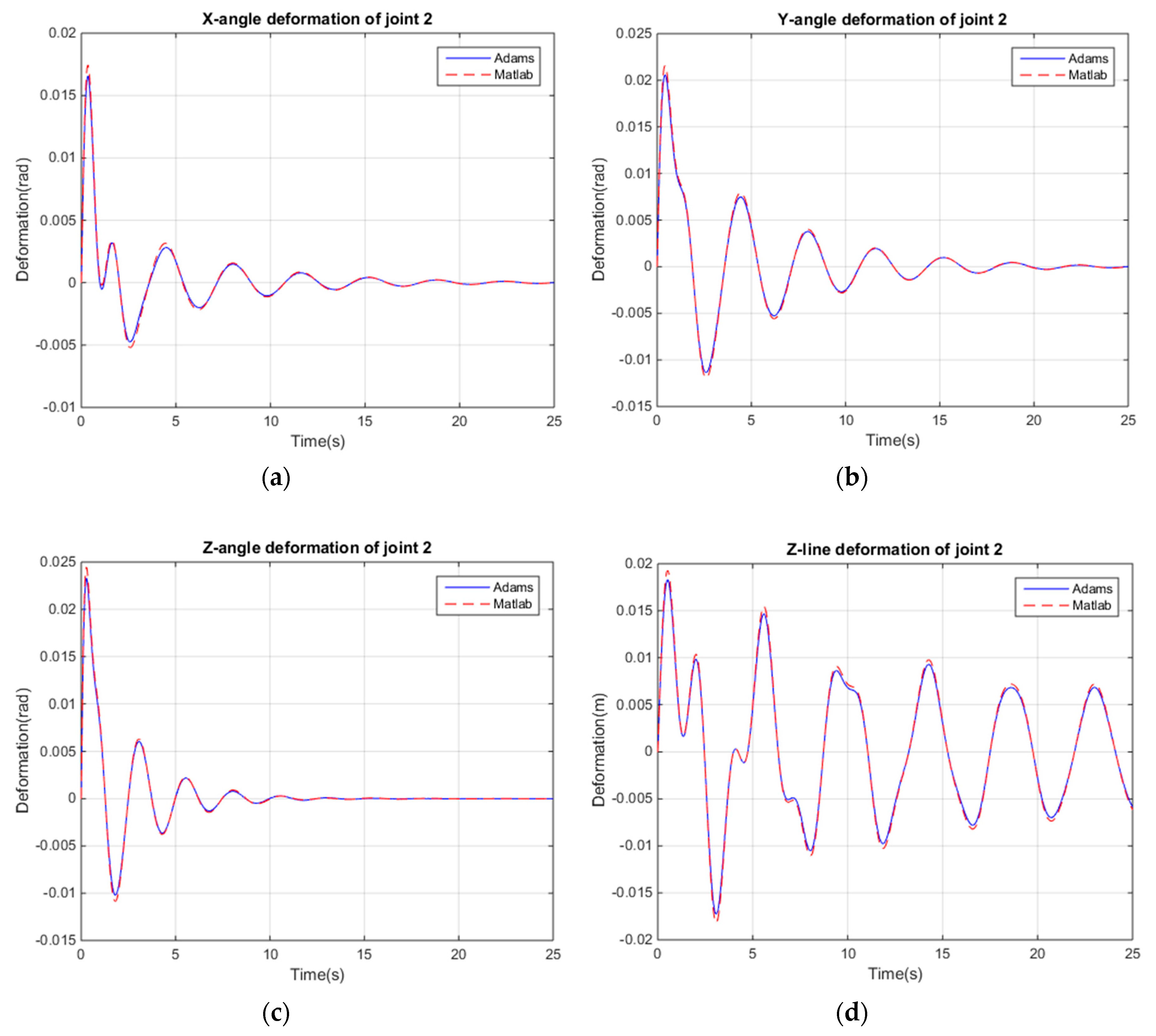
5.2. Spatially Six-Dimensional Collision

In this section, as shown in Figure 11, the dynamic simulations of a space-borne manipulator subjected to a six-dimensional collision are performed. The attitude curves of the floating base under three modes, i.e., rigidity, spring without damping, and spring with damping, are shown, respectively. In addition, the force/torque curves of the floating base under two modes, i.e., spring without damping and spring with damping, are obtained specially. This simulation can be helpful to propose a beneficial method for stabilizing the base attitude by using decentralized damping.
Specific simulation parameters are as follows. Instantaneous impact force/torque existing at the end of manipulator are F = (Fx, Fy, Fz) = (50, 50, 50) N and M = (Mx, My, Mz) = (50, 50,50) N m , and the duration is 0.01 s. Mass of base is 200 kg. Inertia moments of the base are Ix = Iy =53.3 kg m 2 and Iz = 66.7 kg m 2 . Mass of each segment is 8 kg. Inertia moments of each segment are Ix = Iy =5 kg m 2 and Iz = 2.5 kg m 2 . Elastic coefficients of the damper are fwx = fwy = fwz= 40 N m rad 1 and fz = 40 N m 1 . The damping coefficients loaded in the soft-contact joint are based on the adjustment range of the damper, which is 0–5 N·s·m−1(N·s·rad−1), and the decoupled damping coefficients are shown in Table 1.
As shown in Figure 12 and Figure 13, the simulation results of the manipulator with the soft-contact joint are carried out. “Spring without damping” means that the decoupled damping coefficients are zero, “spring with damping.1” and “spring with damping.2” mean that the decoupled damping coefficients are the ones shown in Table 1, and “rigidity” means that all the joints are rigid.
As shown in Figure 12, it can be seen that the joint deformations calculated by Adams is basically consistent with the simulation results of MATLAB. It can be seen that the velocity and angular velocity of the floating base are abruptly changed when subjected to a spatially six-dimensional collision in rigidity mode, and then the gradual changes occur. Under the mode of spring without damping, abrupt changes in the linear velocity and angular velocity of the floating base can be avoided, but there is existing long-term undesirable oscillation. Under the mode of spring with damping, not only the abrupt changes of the velocity and angular velocity of the floating base can be avoided, but the convergence velocity of the amplitude increases with the damping value increasing. For example, the linear velocity and angular velocity of the floating base can be stabilized within 20 seconds under the condition of damping 2#. On the contrary, it takes much more time (i.e., more than 50 seconds) to stabilize under the condition of damping 1#. It can be deduced that the spatial collision momentum is absorbed by decoupled dampers, and a part of the kinetic energy of the captured target can be converted into the internal energy of the damper. By setting different damping coefficients, the convergence time of the vibration can be adjusted.
Under the rigid-collision conditions, the impact force/torque on the base is equal to the force/torque at the end of the manipulator. This means the peak value is 50 N/N·m, and the durations are only 0.01 second. Through the comparative analysis from Figure 13, it can be seen that, under the mode of spring without damping, the contact force/moments of the floating base are small, and then, the oscillation continues. When the damping is introduced, the instantaneous moment/force of the floating base can rapidly convergence, with the damping value increasing. It can be found that the developed soft-contact joint not only can buffer the instantaneous force/torque introduced by docking collision but can unload the force/torque by decoupled dampers.
It can be seen from Figure 14 and Figure 15 that the joint deformations calculated by the Adams simulation is basically consistent with the simulation results of MATLAB. In the Adams environment, the centroids of the manipulator arms and the base are slightly offset due to the existence of the model joint connector, so it is slightly different from the MATLAB theoretical model, but it can be acceptable that there are subtle differences in the calculation results under MATLAB and Adams. Moreover, all joint movements can converge under the action of damping, and this can provide the foundation for the attitude control design of the floating base. From the above simulation results, the developed soft-contact joint is helpful to avoid the instability of the base and convenient for the attitude control of the floating base.

6. Conclusions

A novel soft-contact joint with decoupled dampers was developed to buffer and unload the compact momentum from spatial collisions. Considering a series-wound soft-capture manipulator with multi-joints, the generalized dynamics equations are established by using the Kane approach. Both the benefits of soft-contact joints and the effectiveness of the dynamic equations are verified in MATLAB and Adams software by the simulation of a two-joint manipulator. The comparative simulation results show that the transient impulse momentum with a large magnitude can be converted into sinusoidal momentum with a small magnitude, which is beneficial for the dynamic stability of a capturing system. In the future, the stability control method for capturing a manipulator by using multistage decentralized damping could be a valuable research direction.

Author Contributions

Conceptualization, X.Z.; methodology, X.Z.; software, S.X. and X.Z.; validation, C.J. and S.X.; formal Analysis, S.X. and C.J.; investigation, C.J. and G.W.; resources, G.W.; data Curation, G.W. and M.C.; writing—original draft preparation, X.Z. and S.X.; writing—review and editing, C.J. and M.C.; visualization, C.J.; supervision, X.Z.; project administration, M.C.; and funding acquisition, X.Z. and M.C. All authors have read and agreed to the published version of the manuscript.

Funding

This work was supported by the National Natural Science Foundation of China (51875046 and 61733001), Beijing Natural Science Foundation (3202021) and China Scholarship Council (201906475018).

Conflicts of Interest

The authors declare no conflicts of interest.

References

  1. Pairot, J.M.; Frezet, M.; Tailhades, J. European rendezvous and docking system. Acta Astronaut. 1992, 28, 31–42. [Google Scholar] [CrossRef]
  2. Feng, F.; Liu, Y.W.; Liu, H.; Cai, H.G. Development of space end-effector with capabilities of misalignment tolerance and soft capture based on tendon–sheath transmission system. J. Cent. South. Univ. 2013, 20, 3015–3030. [Google Scholar] [CrossRef]
  3. Olivieri, L.; Francesconi, A. Design and test of a semiandrogynous docking mechanism for small satellites. Acta Astronaut. 2016, 122, 219–230. [Google Scholar] [CrossRef]
  4. Boesso, A.; Francesconi, A. ARCADE small–scale docking mechanism for micro–satellites. Acta Astronaut. 2013, 86, 77–87. [Google Scholar] [CrossRef]
  5. Barbetta, M.; Boesso, A.; Branz, F.; Carron, A.; Olivieri, L.; Prendin, J.; Rodeghiero, G.; Sansone, F.; Savioli, L.; Spinello, F.; et al. ARCADE-R2 experiment on board BEXUS 17 stratospheric balloon. CEAS Space J. 2015, 7, 347–358. [Google Scholar] [CrossRef]
  6. Liu, Y.; Yao, Y.A.; He, Y.Y. Design and research of topological 3–RSR polyhedron docking mechanism. Manned Spacefl. 2018, 24, 61–66. [Google Scholar]
  7. Zhang, X.; Huang, Y.Y.; Chen, X.Q. Analysis and design of parameters in soft docking of micro/small satellites. Sciece China (Inf. Sci.) 2017, 5, 51–64. [Google Scholar] [CrossRef]
  8. Li, L.Q.; Shao, G.B.; Zhou, D.K.; Wang, J.X. Design and analysis of a long–stroke and miniaturized docking mechanism. Manned Spacefl. 2016, 22, 758–765. [Google Scholar]
  9. Liu, X.; Lu, Y.; Zhou, Y.; Yin, Y.H. Prospects of using a permanent magnetic end effector to despin and detumble an uncooperative target. Adv. Space Res. 2018, 61, 2147–2158. [Google Scholar] [CrossRef]
  10. Yoshida, K.; Sashida, N.; Kurazume, R.; Umetani, Y. Modeling of collision dynamics for space free-floating links with extended generalized inertia tensor. In Proceedings of the 1992 IEEE International Conference on Robotics and Automation, Nice, France, 12–14 May1992; pp. 899–904. [Google Scholar]
  11. Yoshida, K.; Sashida, N. Modeling of impact dynamics and impulse minimization for space robots. In Proceedings of the 1993 IEEE/RSJ International Conference on Intelligent Robots and Systems (IROS ’93), Yokohama, Japan, 26–30 July 1993; pp. 2064–2069. [Google Scholar]
  12. Wee, L.B.; Walker, M.W. On the dynamics of contact between space robots and configuration control for impact minimization. IEEE Trans. Robot. Autom. 1993, 9, 581–591. [Google Scholar]
  13. Nenchev, D.N.; Yoshida, K.; Vichitkulsawat, P.; Uchiyama, M. Reaction null–space control of flexible structure mounted manipulator systems. IEEE Trans. Robot. Autom. 1999, 15, 1011–1023. [Google Scholar] [CrossRef] [Green Version]
  14. Nenchev, D.N.; Yoshida, K. Impact analysis and post–impact motion control issues of a free–floating space robot subject to a force impulse. IEEE Trans. Robot. Autom. 1999, 15, 548–557. [Google Scholar] [CrossRef]
  15. Cong, P.C.; Zhang, X. Preimpact configuration analysis of a dual–arm space manipulator with a prismatic joint for capturing an object. Robotica 2013, 31, 853–860. [Google Scholar] [CrossRef]
  16. Oki, T.; Nakanishi, H.; Yoshida, K. Time-optimal manipulator control for management of angular momentum distribution during the capture of a tumbling target. Adv. Robot. 2010, 24, 441–466. [Google Scholar] [CrossRef]
  17. Guo, W.H.; Wang, T.S. Pre-impact configuration optimization for a space robot capturing target satellite. J. Astronaut. 2015, 36, 390–396. [Google Scholar]
  18. Chen, X.; Qin, S. Motion Planning for dual-arm space robot towards capturing target satellite and keeping the base inertially fixed. IEEE Access 2018, 6, 26292–26306. [Google Scholar] [CrossRef]
  19. Xu, W.; Yan, L.; Hu, Z.; Liang, B. Area-oriented coordinated trajectory planning of dual-arm space robot for capturing a tumbling target. Chin. J. Aeronaut. 2019, 32, 2151–2163. [Google Scholar] [CrossRef]
  20. Yu, Z.W.; Cai, G.P. Robust adaptive control of a 6-DOF space robot with flexible panels. Int. J. Dyn. Control 2019, 7, 1370–1378. [Google Scholar] [CrossRef]
  21. Xu, W.L.; Yue, S. Pre–posed configuration of flexible redundant robot manipulators for impact vibration alleviating. IEEE Trans. Ind. Electron. 2004, 51, 195–200. [Google Scholar] [CrossRef]
  22. Larouche, B.P.; Zhu, Z.H. Autonomous robotic capture of non–cooperative target using visual servoing and motion predictive control. Auton. Robot. 2014, 37, 157–167. [Google Scholar] [CrossRef]
  23. McCourt, R.A.; de Silva, C.W. Autonomous robotic capture of a satellite using constrained predictive control. IEEE–ASME Trans. Mechatron. 2006, 11, 699–708. [Google Scholar] [CrossRef]
  24. Zhang, L.; Jia, Q.X.; Chen, G. Pre–impact trajectory planning for minimizing base attitude disturbance in space manipulator systems for a capture task. Chin. J. Aeronaut. 2015, 28, 1199–1208. [Google Scholar] [CrossRef] [Green Version]
  25. Chu, M.; Wu, X.Y. Modeling and self–learning soft–grasp control for free–floating space manipulator during target capturing using variable stiffness method. IEEE Access 2018, 6, 7044–7054. [Google Scholar] [CrossRef]
  26. Nguyen, H.; Thai, C.; Sharf, I. Capture of spinning target with space manipulator using magneto rheological damper. In Proceedings of the AIAA Guidance, Navigation, and Control Conference, Toronto, ON, Canada, 2–5 August 2010; pp. 1–12. [Google Scholar]
  27. Balamurugan, L.; Jancirani, J.; Eltantawie, M.A. Generalized magnetorheological (MR) damper model and its application in semi–active control of vehicle suspension system. Int. J. Automot. Technol. 2014, 15, 419–427. [Google Scholar] [CrossRef]
  28. Yu, Z.W.; Liu, X.F.; Cai, G.P. Dynamics modeling and control of a 6-DOF space robot with flexible panels for capturing a free floating target. Acta Astronaut. 2016, 128, 560–572. [Google Scholar]
  29. Bian, Y.S.; Gao, Z.H. Nonlinear vibration absorption for a flexible arm via a virtual vibration absorber. J. Sound Vib. 2017, 399, 197–215. [Google Scholar] [CrossRef]
  30. Bian, Y.S.; Gao, Z.H.; Lv, X.; Fan, M. Theoretical and experimental study on vibration control of flexible manipulator based on internal resonance. J. Vib. Control 2018, 24, 3321–3337. [Google Scholar] [CrossRef]
Figure 1. Three-dimensional model of the soft-contact joint.
Energies 13 01530 g001
Figure 2. Structural block diagram of the soft-contact joint.
Energies 13 01530 g002
Figure 3. Overall structure of the soft-contact joint.
Energies 13 01530 g003
Figure 4. Block diagram of the dual working modes transmission.
Energies 13 01530 g004
Figure 5. Block diagram of the soft-contact principle. (a) Block diagram of the buffer and unloading of spatial collision. (b) The representative force (moment) diagram of two consecutive joints.
Energies 13 01530 g005aEnergies 13 01530 g005b
Figure 6. Novel joint and generalized model of the manipulator. (a) Joint structure with six-dimensional damping. (b) Generalized model of the manipulator with multi-stage damping.
Energies 13 01530 g006
Figure 7. Stress analysis for the kth segment.
Energies 13 01530 g007
Figure 8. Conceptual model of simulation. (a) Structure diagram for MATLAB. (b) Adams model.
Energies 13 01530 g008
Figure 9. Schematic diagram of six unidirectional collision forces.
Energies 13 01530 g009
Figure 10. Vibration displacements of joints in a single-direction collision. (a) Vibration displacements in a single X-line collision. (b) Vibration displacements in a single X-angle collision. (c) Vibration displacements in a single Y-line collision. (d) Vibration displacements in a single Y-angle collision. (e) Vibration displacements in a single Z-line collision. (f) Vibration displacements in a single Z-angle collision.
Energies 13 01530 g010aEnergies 13 01530 g010bEnergies 13 01530 g010cEnergies 13 01530 g010dEnergies 13 01530 g010e
Figure 11. Schematic diagram of six unidirectional collision forces.
Energies 13 01530 g011
Figure 12. The curves of linear and angular velocity of the base. (a) X-line velocity. (b) X-angle velocity. (c) Y-line velocity. (d) Y-angle velocity. (e) Z-line velocity. (f) Z-angle velocity.
Energies 13 01530 g012aEnergies 13 01530 g012bEnergies 13 01530 g012cEnergies 13 01530 g012dEnergies 13 01530 g012e
Figure 13. The curves of the torques and the force of the base. (a) X-angle torque. (b) Y-angle torque. (c) Z-angle torque. (d) Z-line force.
Energies 13 01530 g013aEnergies 13 01530 g013b
Figure 14. Vibration displacements of joint 1. (a) X-angle vibration displacement. (b) Y-angle vibration displacement. (c) Z-angle vibration displacement. (d) Z-line vibration displacement.
Energies 13 01530 g014
Figure 15. Vibration displacements of joint 2. (a) X-angle vibration displacement. (b) Y-angle vibration displacement. (c) Z-angle vibration displacement. (d) Z-line vibration displacement.
Energies 13 01530 g015
Table 1. Value of representative the damping coefficient.
ItemParameter
1#1.0 N·s·m−1(N·s·rad−1)
2#5.0 N·s·m−1(N·s·rad−1)

