Article

Application of the Feedback Linearization in Maximum Power Point Tracking Control for Hydraulic Wind Turbine

1
Hebei Heavy Machinery Fluid Power Transmission and Control Laboratory, Yanshan University, Qinhuangdao 066004, China
2
School of Mechanical Engineering, Yanshan University, Qinhuangdao 066004, China
3
Nanjing Institute of Technology, Nanjing 211167, China
*
Author to whom correspondence should be addressed.
Energies 2020, 13(6), 1529; https://doi.org/10.3390/en13061529
Submission received: 11 February 2020 / Revised: 5 March 2020 / Accepted: 17 March 2020 / Published: 24 March 2020
(This article belongs to the Collection Wind Turbines)

Abstract

:
Taking the hydraulic wind turbine as the research object, the method is studied to improve the utilization ratio of wind energy for hydraulic wind turbine, when the wind speed is lower than the rated wind speed. The hydraulic fixed displacement pump speed and generating power can be used as control output to realize the maximum power point tracking control. The characteristics of the maximum power point tracking control are analyzed for hydraulic wind turbine, and the hydraulic output power is taken as control output based on the comprehensive performance requirements. Because the hydraulic wind turbine is a strong multiplication nonlinear system, the system is globally linearized based the feedback linearization method, and the maximum power point tracking control law is obtained. The simulation and experiment results show that the system has good dynamic performance with the proposed control law. The control provides theoretical guidance for optimal power tracking control law application for hydraulic wind turbine.

1. Introduction

Wind energy is a vast renewable energy resource being increasingly tapped by wind turbines which are growing in number and size. Conventional wind turbines transmissions consist of a mechanical gearbox and high-speed generator, or sometimes direct drive low-speed generators are used as described in [1]. But these two traditional transmission schemes have some disadvantages, such as high cost and high failure rate. In order to reduce the cost and improve the reliability, hydrostatic transmission has been proposed in [2,3,4]. Thus, the power captured by the turbine rotor will be transmitted to the generator through the hydrostatic transmission, and the generator can be flexibly installed, either in the nacelle of the wind turbine or installed on the ground driven by hydraulic pipelines, which greatly reduces the difficulty of installation and maintenance. Benefits of the hydraulic wind turbine (HWT) are that the hydrostatic transmission is inherently more compliant than the mechanical transmission, which makes it more reliable in face of shock loading, and the transmission ratio is adjustable, so the system does not need additional frequency conversion devices to coordinate wind turbine speed and power grid frequency. Meanwhile, with the development of digital hydraulic technology, the low part-load efficiency of conventional hydraulics is solved [5].
In order to improve the efficiency of wind energy utilization, scholars at home and abroad have done a lot of research on the maximum power point tracking (MPPT) control for HWT. An optimal H∞ ring forming pressure controller was designed for a mechano-hydraulic hybrid wind turbine, which can accurately track the optimal load pressure in [6]. The small signal linearization and variable gain proportional integral differentiation (PID) were combined to solve the problem of inconsistent power response, and the speed control loop is used to optimize the MPPT strategy in [7]. A sensorless double integral sliding mode controller was designed to achieve maximum power extraction under the condition of large parameter uncertainty and nonlinearity for hydrostatic tidal turbine in [8]. A PID controller and a sliding mode controller were applied for speed control to track a predefined speed in [9]. To track the maximum power point, a takagi-sugeno (TS) fuzzy model was proposed for the HWT with two variable displacement pumps and a fixed displacement motor, and a parameter varying model predictive control (PVMPC) approach was designed in [10]. Shengquan Li proposed a combined model predictive control strategy to achieve the purpose of MPPT control for HWT in [11]. SP Mulders proposed an implementation, model-free, gradient-based and extremum seeking control optimization strategy to achieve an average maximum power increase in [12]. M, Deldar designed a decentralized control configuration to collect the maximum energy without directly measuring the wind speed in [13]. A digital hydrostatic drive solution was introduced in the HWT to largely utilize the energy captured by the rotor in [14], and the kW2 control law combined with digital hydrostatic method was proposed to improve HWT energy production. Active disturbance rejection controller (ADRC) control method was introduced to achieve HWT MPPT control, and the pump speed was taken as the control output in [15]. However, the MPPT control smoothness needed to be further improved. The frequency control and the MPPT control rely on the mechanical torque adjustment on the hydraulic motor that was coupled with the generator in [16]. A MPPT control strategy based on the tip speed ratio (TSR) was adopted for the 600 kW hydraulic energy storage wind turbine, and the maximum power tracking performance was simulated and analyzed by subjecting to turbulent speed condition in [17].
The above-mentioned researches on MPPT control methods verify the proposed controller effectiveness from a theoretical point view and provide a certain reference. However, according to the HWT with a fixed displacement pump and a variable displacement motor, it is also necessary to explore a MPPT controller. Therefore, based on the HWT working principle, a state space model is established. Because the hydraulic main transmission system has strong nonlinearity, wind has randomness and volatility, and sometimes the fluctuation range is large, the feedback linearization method can rid the system of small signal linearization limitation, and the analysis and synthesis of the system in a large range is realized [18]. Thus, the feedback linearization method is adopted to conduct the MPPT controller.
The paper is organized as follows: the HWT working principle and the requirements for MPPT control are introduced in Section 2. The HWT mathematical model is established in Section 3. In Section 4, the feedback linearization method is used to globally linearize the system, and the MPPT controller is proposed with the output of power. In Section 5, the simulation results are carried out under the different conditions, and the experiment results are also carried out based on the 24 kW HWT experiment platform. Finally, conclusions are drawn in Section 6.

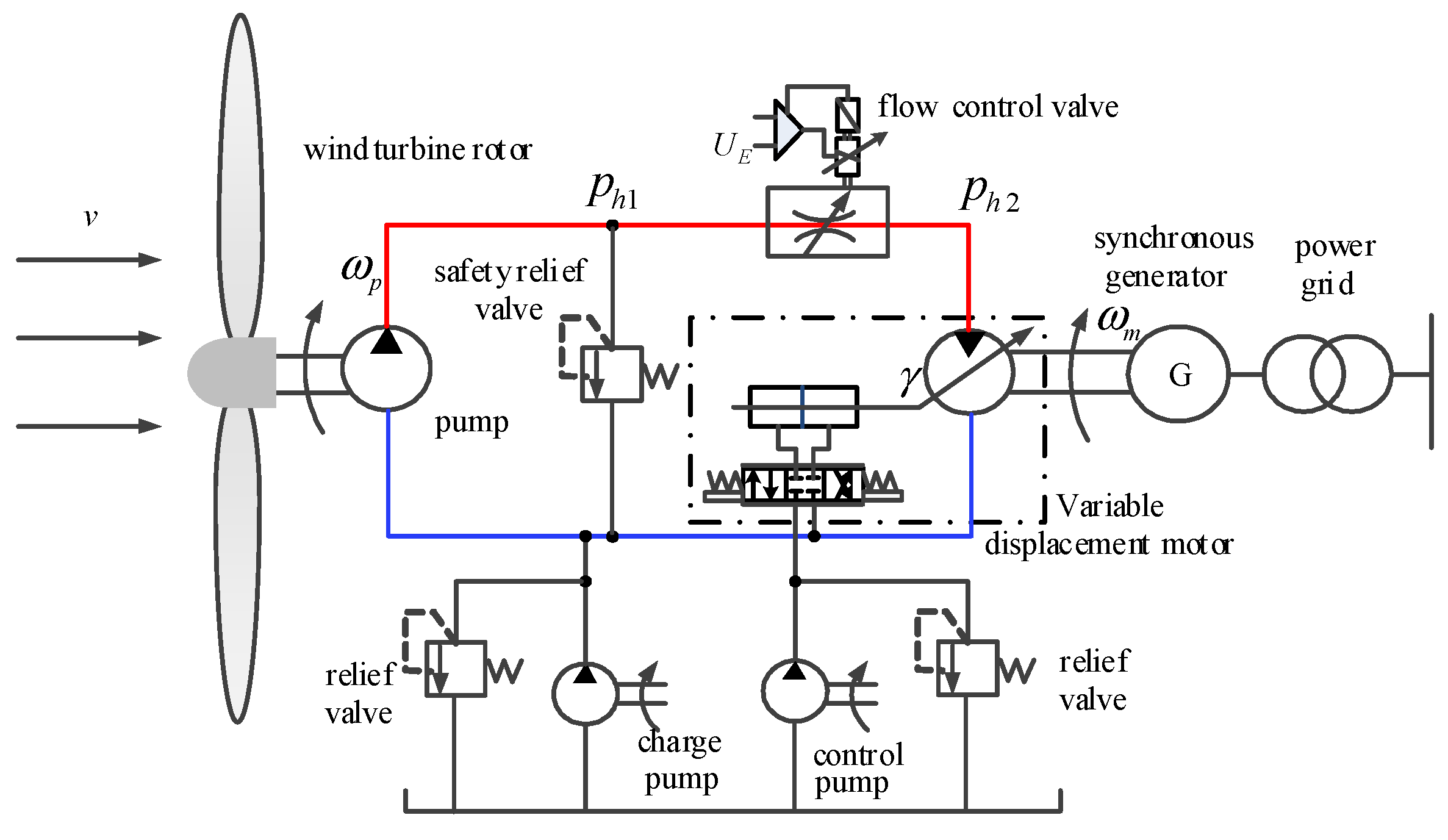
2. Description of the HWT

2.1. HWT Working Principle

HWT is mainly composed of a rotor, a fixed displacement pump, a variable displacement motor and a synchronous generator. An inverter for frequency conversion is not required. The rotor and the pump are coaxially connected, and the pump supplies high pressure oil to the motor, so the fluctuation of the wind speed tends to affect the motor speed [19,20]. The motor and the generator are also coaxially connected, and the motor and generator speed are controlled by changing the motor displacement. When the synchronous generator is stable within the required speed range (1500 r/min ± 6 r/min), it can be connected to the grid for power generation. At the same time, the charge pump provides hydraulic oil for the low-pressure pipeline, the control pump provides hydraulic oil for control pipeline of the variable displacement motor, and the safety relief valve and relief valve are used for system protection. A schematic diagram of the HWT is shown in Figure 1.

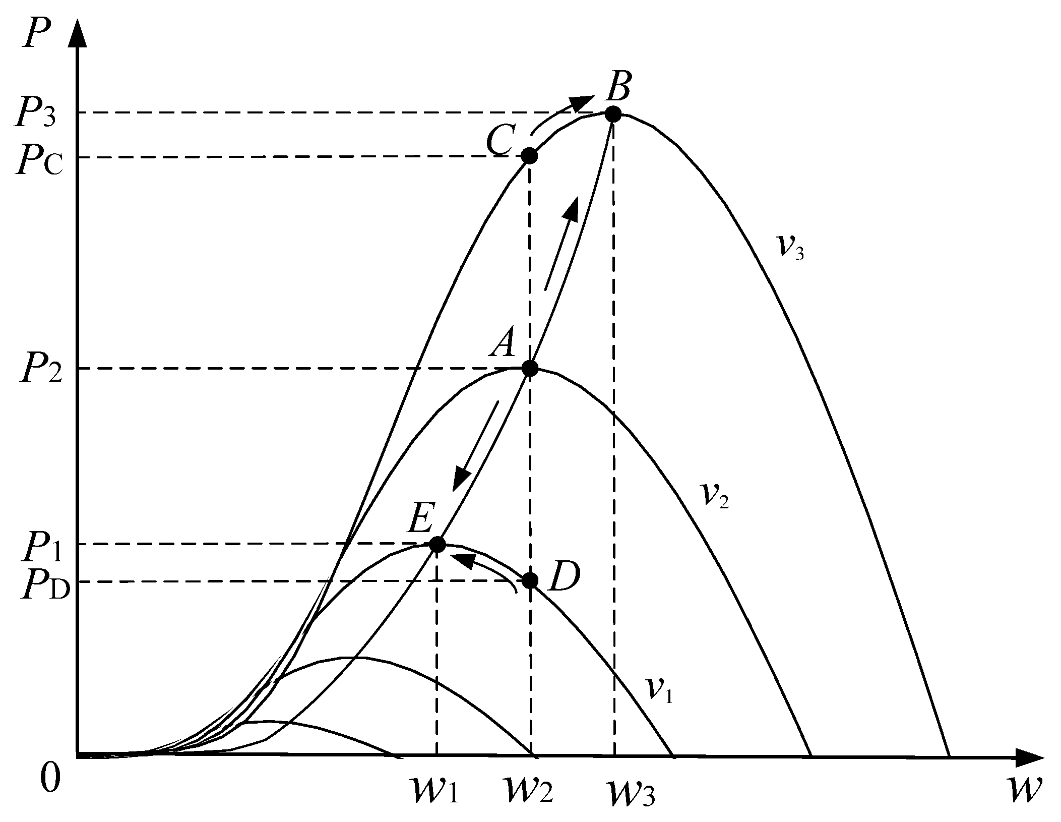
2.2. Control Effects of MPPT

The maximum wind power captured by the wind turbine under the demand wind speed [21] is expressed as
P r max = 1 2 ρ π R 2 v 3 C p max
The rotor speed is related to the wind speed, and the rotor speed is expressed as
ω = v λ o p t R
From the Equations (1) and (2), the relationship between the captured maximum wind power and the rotor speed (the pump speed) can be expressed as
P r max = ρ π R 5 C p max 2 λ o p t 3 ω 3 = K P ω 3
The principle of the MPPT method for direct generation power control is shown in Figure 2, and the tracking process is expressed as follows:
Assuming wind speed v1 < v2 < v3, E, A, and B are the maximum power points at the three kinds of wind speed, respectively. The initial wind speed is v2, and initially the wind turbine works stably at point A, which is the maximum power point at wind speed v2.
When the wind speed increases from v2 to v3, since the rotor speed cannot change suddenly, the input power is the power PC corresponding to point C, and the power value is the power P2 corresponding to point A. Since the input power PC is always greater than the generating power P2 before point B, the rotor will accelerate. As the rotor speed increases, the input power moves from point C to the maximum power point B along the power characteristic curve of v3; the actual generating power moves from point A to point B along the demand value of the generating power (the optimal power curve). The rotor input power is equal to the demand power at point B, and the system is re-balanced. At this point, the MPPT process is completed when the wind speed increases from v2 to v3.
In a similar way, when the wind speed decrease from v2 to v1, since the rotor speed cannot change suddenly; the input power is the power PD corresponding to point D, and the power value is the power P2 corresponding to point A. Since the input power PD is always less than the generating power P2 before point E, the rotor will slow down. As the rotor speed decreases, the input power moves from point D to the optimal power point E along the power characteristic curve of v1. The actual generating power moves from point A to point E along the demand value of the generating power (the optimal power curve). The input power is equal to the demand value of power generation at point E, and the system is re-balanced. At this point, the MPPT process is completed when the wind speed decreases from v2 to v1.
Based on the above principle analysis, the MPPT method of direct generation power control can automatically track the wind turbine to the maximum power point. The rapidity and accuracy of the MPPT process is taken into account.

3. The Mathematical Model of the Hydraustatic Transmission

3.1. The Pump Model

The pump shaft torque is related to the pressure, and the torque is expressed as
T p = D p p h 1 η m e c h , p
The difference between the rotor and pump torque accelerates the combined inertia and overcomes viscous friction. The torque balance equation is expressed as
T v ( ω p , v ) T p = J p d ω p d t + B p ω p
Flow continuity equation of the fixed displacement pump is expressed as
Q p = D p ω p C t 1 p h 1
From the Equations (4)–(6), the state equation of the pump speed can be expressed as
ω ˙ p = 1 J p ( T r D p p h 1 η m e c h , p B p ω p )

3.2. The Motor Model

Similarly, the motor output torque is related to pressure, and the torque is expressed as
T m = D m p h 2 η m e c h , m = K m γ p h 2 η m e c h , m
The difference between the motor and generator torque accelerates the motor inertia and overcomes the viscous friction. The torque balance equation is expressed as
T m T L = J m d ω m d t + B m ω m
And the variable motor flow continuity equation is expressed as
Q m = D m ω m + C t 2 p h 2
From the Equations (8)–(10), the state equation of the motor speed is
ω ˙ m = 1 J m ( K m γ p h 2 η m e c h , m B m ω m T L )

3.3. The Flow Control Valve Model

The flow through the proportional flow control valve is expressed as
Q b l = K U E

3.4. The Hose Model

The oil flows between pump and motor inside a hose, and the general equation for the additional flow caused by oil compressibility and hose compliance is expressed as
Q c = V β e d p h d t
The proportional flow control valve divides the high-pressure line into two parts, one is the pump to the flow control valve, with volume V1, and the other part is the flow control valve to the motor, with volume V2.

3.5. The Hydraulic Transmission System State Space Model

The compressibility flow between the pump and the flow control valve is expressed as
Q c 1 = Q p Q b l = D p ω p C t 1 p h 1 K U E
The compressibility flow between the flow control valve and the motor is expressed as
Q c 2 = Q b l Q m = K U E D m ω m C t 2 p h 2
To establish the state space model of the main transmission system for the HWT, the following assumptions need to be made:
(1)
The pressure in the low-pressure line is a constant.
(2)
The leakage coefficient, the viscous damping coefficient and the bulk modulus of the oil are the fixed values, which do not change with temperature or other factors.
(3)
The pressure loss in the hydraulic lines is ignored.
(4)
The pump mechanical efficiency η mech , p is designed 1.
The system state space model is obtained by combining the Equations (7), (11)–(15).
{ ω ˙ p = B p J p ω p D p J p p h 1 + 1 J p T v ( ω p , v ) p ˙ h 1 = D p β V 1 ω p C t 1 β V 1 p h 1 K β U E V 1 p ˙ h 2 = K β U E V 2 C t 2 β V 2 p h 2 K m β ω m V 2 γ ω ˙ m = B m J m ω m + K m p h 2 J m γ 1 J m T L
Due to the MPPT control process, the grid-connected speed control has been completed, and the motor speed is constant; that is, ω m = 1500 r / min . Moreover, the proportional throttle valve opening is open. Thus, the system status values are the pump speed and the pressure between the pump and variable displacement motor. The state equation during power tracking can be expressed as
{ ω ˙ p = B p J p ω p D p J p p h + 1 J p T r ( ω p , v ) p ˙ h = D p β V ω p C t β V p h K m ω md β V γ
The state variables is define as x 1 = ω p ,   x 2 = p h , and the system control input is u = γ . Therefore, the system state space model after grid-connection can be expressed as
{ x ˙ 1 = B p J p x 1 D p J p x 2 + 1 J p T r ( x 1 , v ) x ˙ 2 = D p β V x 1 C t β V x 2 K m ω md β V u
The system model is rewritten into affine nonlinear form x ˙ = f ( x ) + g ( x ) u , the system state space model after grid grid-connection can be expressed as
f ( x ) = [ B p J p D p J p 1 J p D p β V C t β V 0 ] [ x 1 x 2 T r ( x 1 , v ) ]
g ( x ) = [ 0 K m ω md β V ]

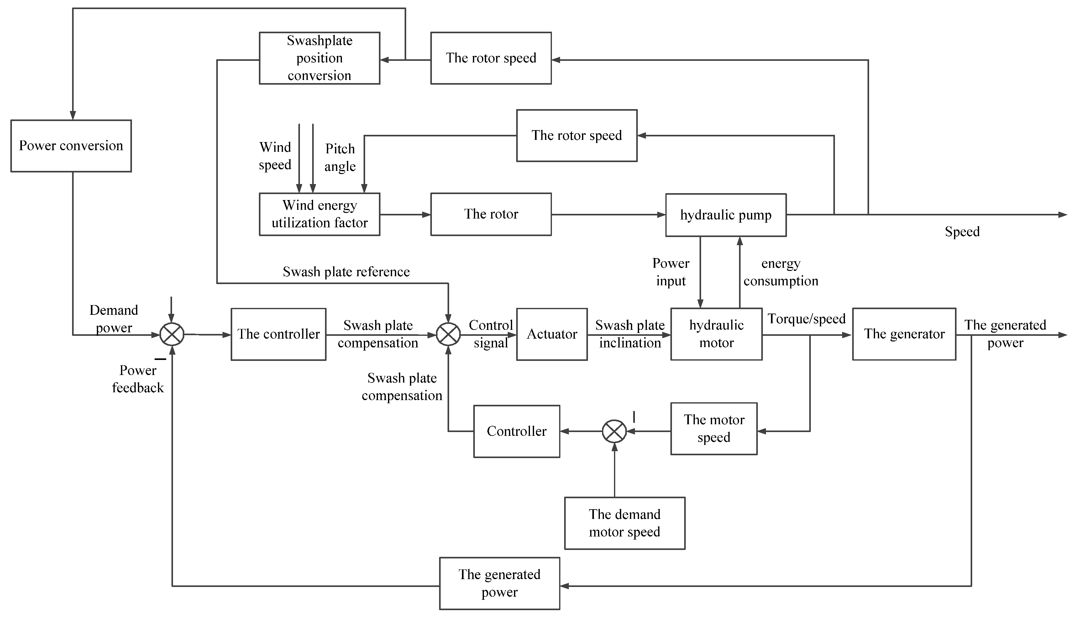
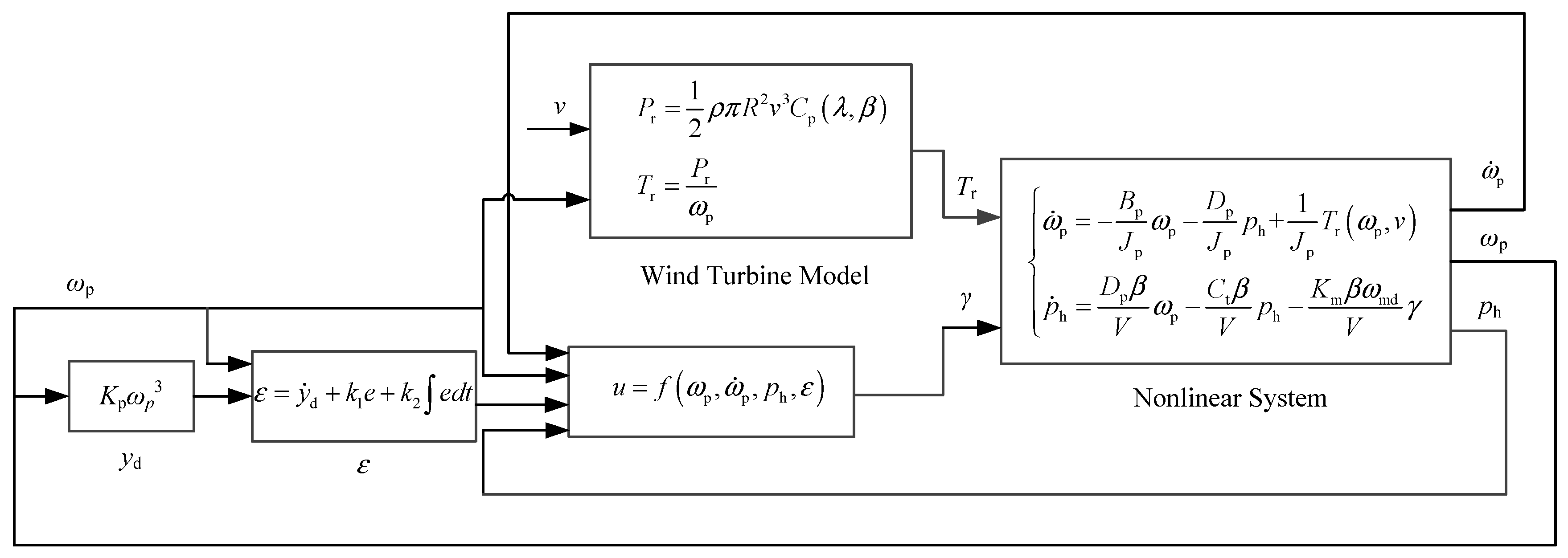
4. The MPPT Controller Based on Feedback Linearization Method

4.1. Control Thoughts

In the MPPT method for direct power generation control, the control system mainly includes three control loops, which are the motor displacement reference control loop, the motor speed control loop, and the power control loop. Among the three control loops, the motor displacement reference control loop is calculated from the fixed displacement pump speed based on the traffic conservation, and the purpose of the motor displacement reference control loop is to make the variable motor work at the excitation synchronous speed. The motor speed control loop is the motor displacement fine-tuning amount, formed by the deviation between the demand synchronous speed (1500 r/min) and the actual motor speed. The function of the motor speed control loop is to control the variable motor to work precisely at the synchronous speed and achieve quasi-synchronous grid connection. Power control loop is the reference value of the maximum power, which is calculated by the actual pump speed according to the optimum blade tip ratio and the maximum wind energy utilization coefficient. Compared with the actual power, the deviation is formed, and the displacement compensation value is adjusted by the controller. The specific control block diagram is shown in Figure 3.

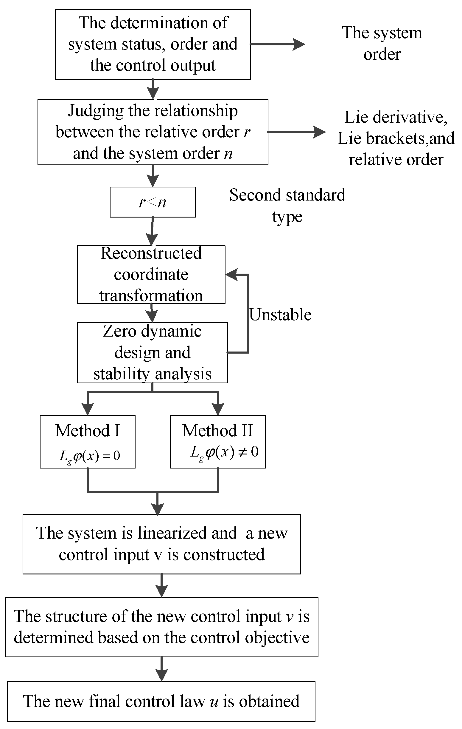
4.2. MPPT Controller Design

The process of solving the system control law using the feedback linearization method is shown in Figure 4 [18,19,20,21,22].

4.2.1. Control Output

The control output is expressed as
y = h ( x ) = D p x 1 x 2 = D p ω p p h

4.2.2. Relative Order

The definition of relative order is as follows: (1) The Lie derivative value of the k-order Lie derivative of the output function h(x) to the vector field F(x) to the vector field F(x) in the neighborhood of x = x0 is zero; that is, L g L f k h ( x ) = 0 . (2) The Lie derivative value of the (r−1)-order Lie derivative (k < r−1) of the output function h(x) to the vector field F(x) to the vector field F(x) in the neighborhood of x = x0 is not zero; that is, L g L f r 1 h ( x ) 0 . Then the relative degree of nonlinear system (18) in x = x0 is defined as r [18,19,20,21,22].
From the equations (17)–(20), according the relevant definition of the Lie derivative, the relative order evaluation expression is
L g L f 0 h ( x ) = K m β ω md D p x 1 V 0
From the expression (22), the relative order r = 1 < 2 , the system cannot be linearized in full state and zero dynamic design is required.
From the above analysis, the system cannot be completely linearized. Therefore, input–output linearization and the zero dynamic design method are adopted to determine the system controller [22].
In the process of zero dynamic design, the system dynamic behavior can be divided into the external dynamics and internal dynamics. The external dynamics are not only required to be stable but also have tracking performance and reject disturbance. The internal dynamics are only required to be stable.

4.2.3. Zero Dynamic Controller Design

The zero dynamics selected in this paper is φ 2 ( x ) = x 1 , the pump speed, which is considered as the internal dynamics. First, a coordinate transformation of the system gives
{ z 1 = φ 1 ( x ) = h ( x ) = D p x 1 x 2 z 2 = η 2 ( x ) = x 1
Thus, the Jacobian matrix of the vector function φ(x) = [z1(x) z2(x)]T at x = x0 is expressed as
J φ = ϕ ( x ) ( x ) | x = x 0 = [ D p x 2 D p x 1 1 0 ]
This is a non-singular at x = x0, so the coordinate transformation is valid.
And then the inverse mapping of z = φ(x) is x = φ−1(z). Therefore, the x can be expressed as
{ x 1 = z 2 x 2 = z 1 D p z 2
From the equations (18) and (25), the final expression of the system in z coordinates can be expressed as
{ z ˙ 1 = D p z 1 D p z 2 ( B p J p z 2 D p J p z 1 D p z 2 + 1 J p T r ( z 2 , v ) ) + D p z 2 ( D p β V z 2 C t β V z 1 D p z 2 ) u z ˙ 2 = B p J p z 2 1 J p z 1 z 2 + 1 J p T r ( z 2 , v )
The system output in the z coordinate system is expressed as
y = z 1
The external state, which is the pump outlet power, is close to zero and in a stable state, that is, z 1 = 0 , z ˙ 1 = 0 . At this point, the equations (26) can be expressed as
z ˙ 2 = B p J p z 2 + 1 J p T r ( z 2 , v )
When the external state is close to zero, the internal state stability is related to the pump external load, and it is irrelevant to u , but all are asymptotically stable. Therefore, the system has zero dynamic stability and can be solved by the controller [23].
After the coordinate transformation and the zero-dynamic design, the HWT MPPT controller can be designed based on the feedback linearization control method. The specific method is to linearize the system in the coordinate system, and the output and the control input of the system are linearly related.
First, the desired control input is constructed as z ˙ 1 = v * . At this point, the system output and the constructed input v * are linearly dependent. The constructed input is expressed as
v * = D p x 2 ( B p J p x 1 D p J p x 2 + 1 J p T r ( x 1 , v ) ) + D p x 1 ( D p β V x 1 C t β V x 2 ) u
Then the system can be linearized as follows:
{ z ˙ 1 = v * z ˙ 2 = B p J p z 2 1 J p z 1 z 2 + 1 J p T v ( z 2 , v )
Thus, the zero dynamics is asymptotically stable, and the whole system is asymptotically stable. That is, the selected coordinate transformation can be used to solve the controller, and the system is in a stable state under the controller.
Thus, the motor control input can be expressed in terms of v*
u = V K m β ω m d D p x 1 ( v [ D p x 2 ( B p J p x 1 D p J p x 2 + 1 J p T v ( x 1 , v * ) ) + D p x 1 ( D p β V x 1 C t β V x 2 ) ] )

4.2.4. Output Reference Design

When the power is taken as control output, the demand maximum power at each wind speed is expressed as
y d = K p ω p 3 = ρ π R 5 C p max 2 λ opt 3 ω p 3

4.2.5. Controller Design

In the control process of the MPPT, theoretically, the system is linearized precisely. However, there will be tracking errors due to model parameters. The closed loop PI control is used to reduce the tracking error.
The tracking error is defined as
e = y d y
and the new control input [24] is expressed as
v * = y ˙ d + k 1 e + k 2 e d t
In (34), the values of k 1 , k 2 are turned according to the control requirements.
The final controller is given by (31) and (34). The controller expressed in terms of physical variables is:
γ = D p ω p C t p h K m ω m d V K m β ω m d D p ω p ( v * D p p h ω ˙ p )
According to the (35), the system states and constructed control inputs are combined linearly to form the control signal for the motor displacement. Through the real-time detection of system states, the calculated control signals are sent to the system to realize the MPPT control.
Comprehensively considering the rapidity, accuracy and stability of the power tracking of the hydraulic wind turbine and combining the effects of the proportional and integral links on the control system, the control parameters are shown in Table 1.

5. Simulation and Experiment Research

5.1. Simulation Platform

A mathematical model, as showed in Figure 5., is established in MATLAB/Simulink@ software. The nonlinear controller accuracy, which is based on the feedback linearization theory, can be verified under different kinds of wind speed. The corresponding parameters of the system are shown in Table 2.

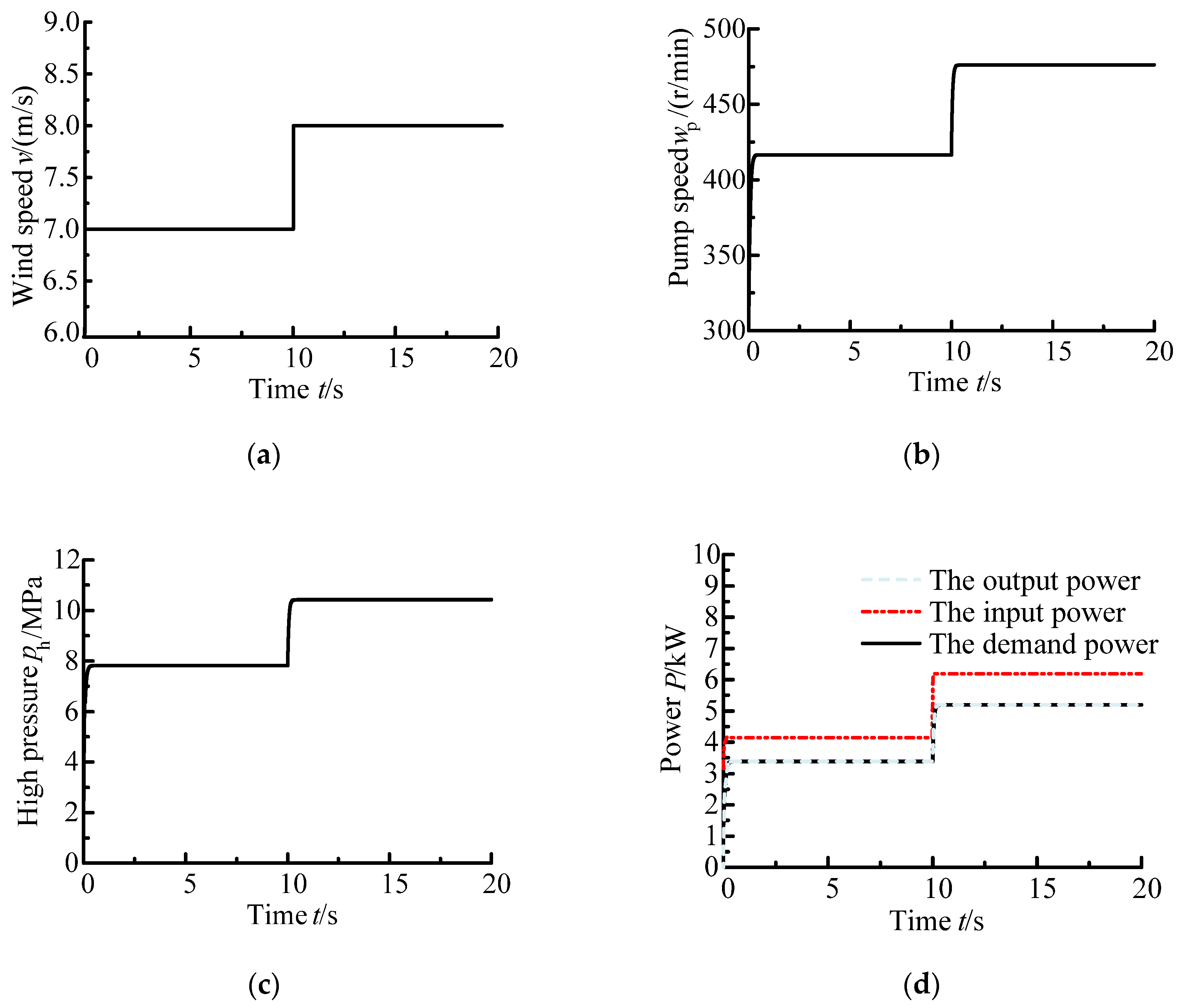
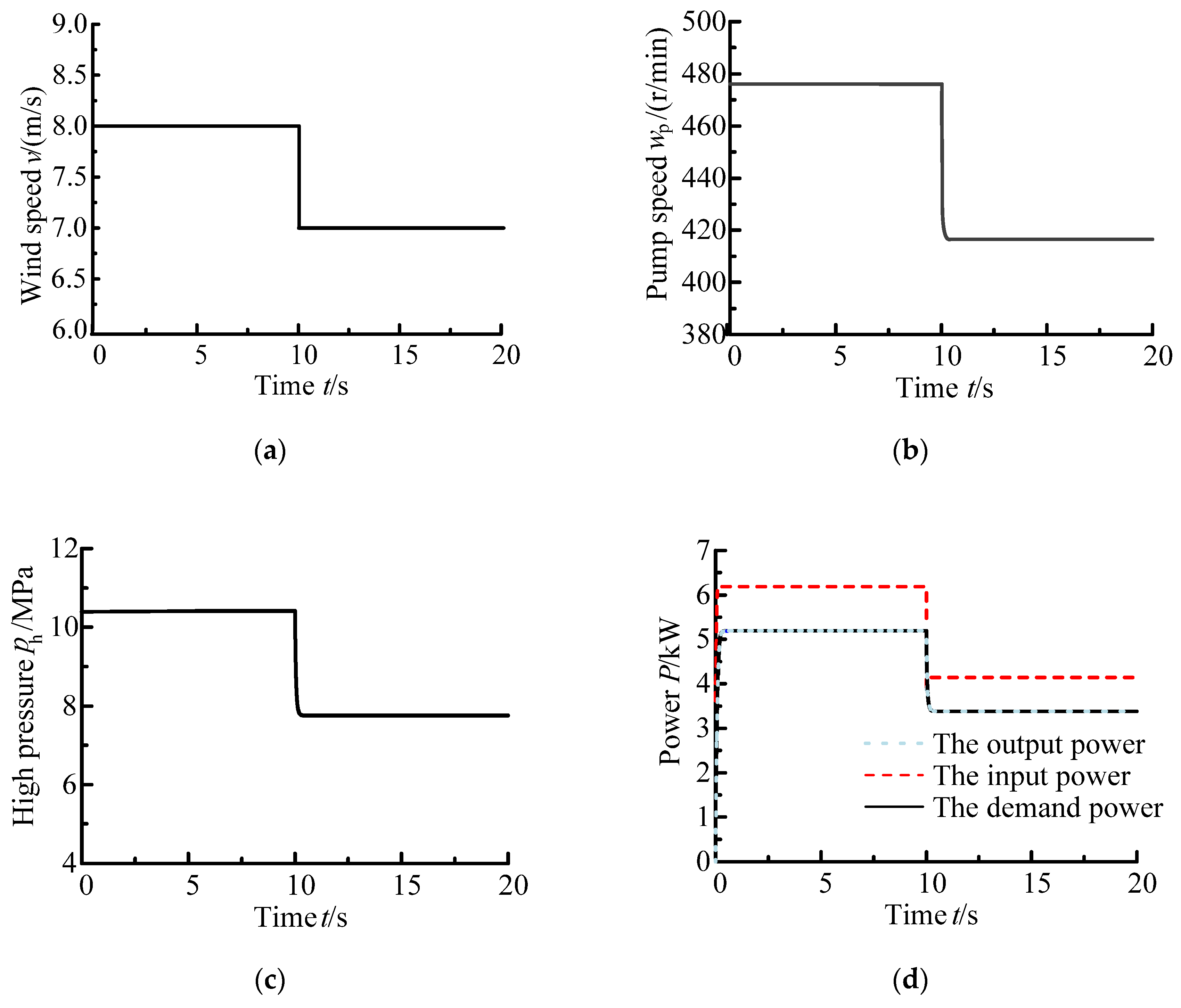
5.2. Simulation Analysis

In order to verify the proposed control method effectiveness, the HWT MPPT control are researched based on the above simulation platform. Under the condition of 7 m/s–8 m/s step wind speed at 10 s, the response characteristics of system are observed during the process of the power tracking, and the specific curves are shown in Figure 6.
Under the condition of 8 m/s–7 m/s step wind speed at 10 s, the response characteristics of system are observed during the process of the power tracking, and the specific curves are shown in Figure 7.
From the results of Figure 6; Figure 7, the pump speed and high pressure change with the step wind speed, and the demand power curve coincides with the output power curve; that is, the output power can track the demand power. The MPPT controller effectiveness is verified. There is a difference between the input wind power and output power, and the difference is 1 kW; the reason is that in the pump–motor system there is transmission efficiency.
There are two main types of energy loss in the process of energy flow conversion, which are the energy lost by the hydraulic transmission system and the energy lost by the generator. Among them, the energy lost by the hydraulic transmission system mainly includes volume loss and oil heating loss, and the energy lost by the generator mainly includes mechanical loss and electromagnetic loss. The wind energy absorbed by the wind turbine cannot be completely converted into electrical energy with these unavoidable energy losses.
Under the conditions of 7 m/s ( ± 0.5 m/s)–8 m/s ( ± 0.5 m/s) in wind speed, the response characteristics of system are observed during the process of the power tracking, and the specific curves are shown in Figure 8.
From the results of Figure 8, the pump speed and high pressure also change with the fluctuated speed, and the demand power curve also coincides with the output power curve; that is, the output power can track the demand power. The motor swing angle is adjusted to achieve the above results, and the MPPT controller effectiveness is verified further. There is a difference between the input wind power and output power; the difference is 1.2 kW, and the reason is that in the pump–motor system there is transmission efficiency.

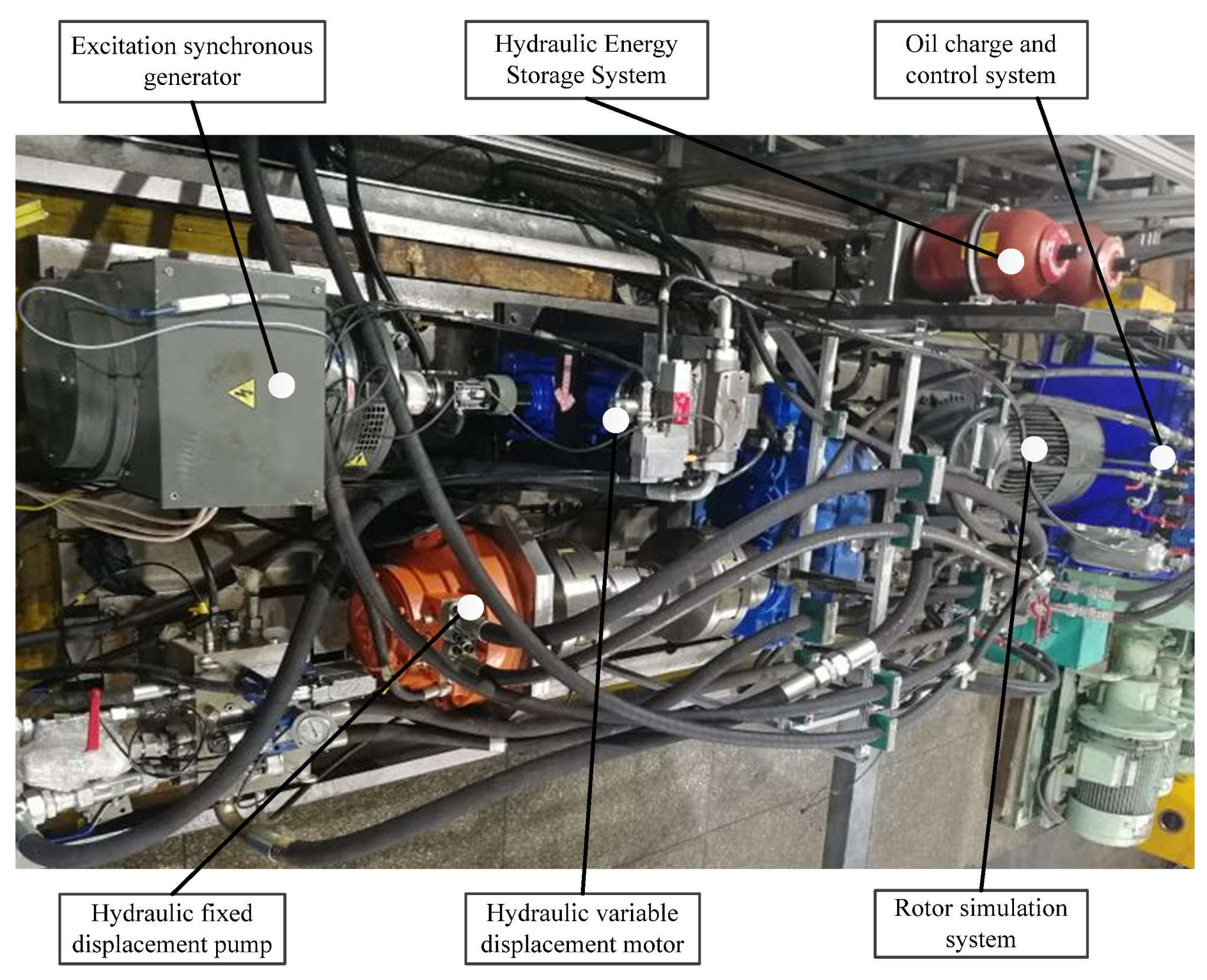
5.3. Experiment Platform

The 24 kW HWT experiment simulation platform is shown in Figure 9. The system major hardware models are shown in Table 3. The experimental platform mainly consists of four parts: wind turbine simulation system, hydraulic transmission system, grid-connected generation system and control system. Among them, the frequency converter is used to control the frequency conversion motor to simulate the wind turbine.

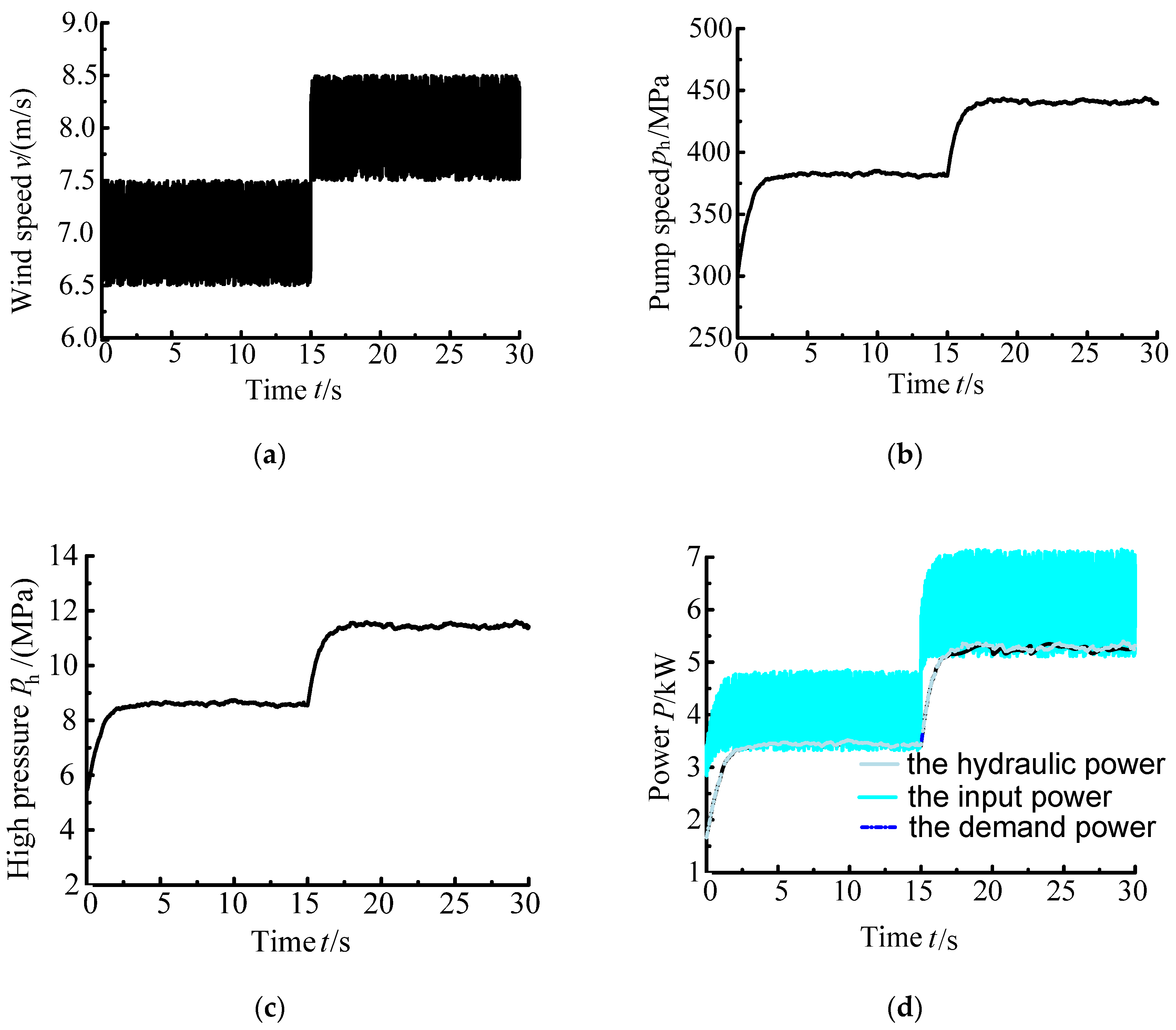
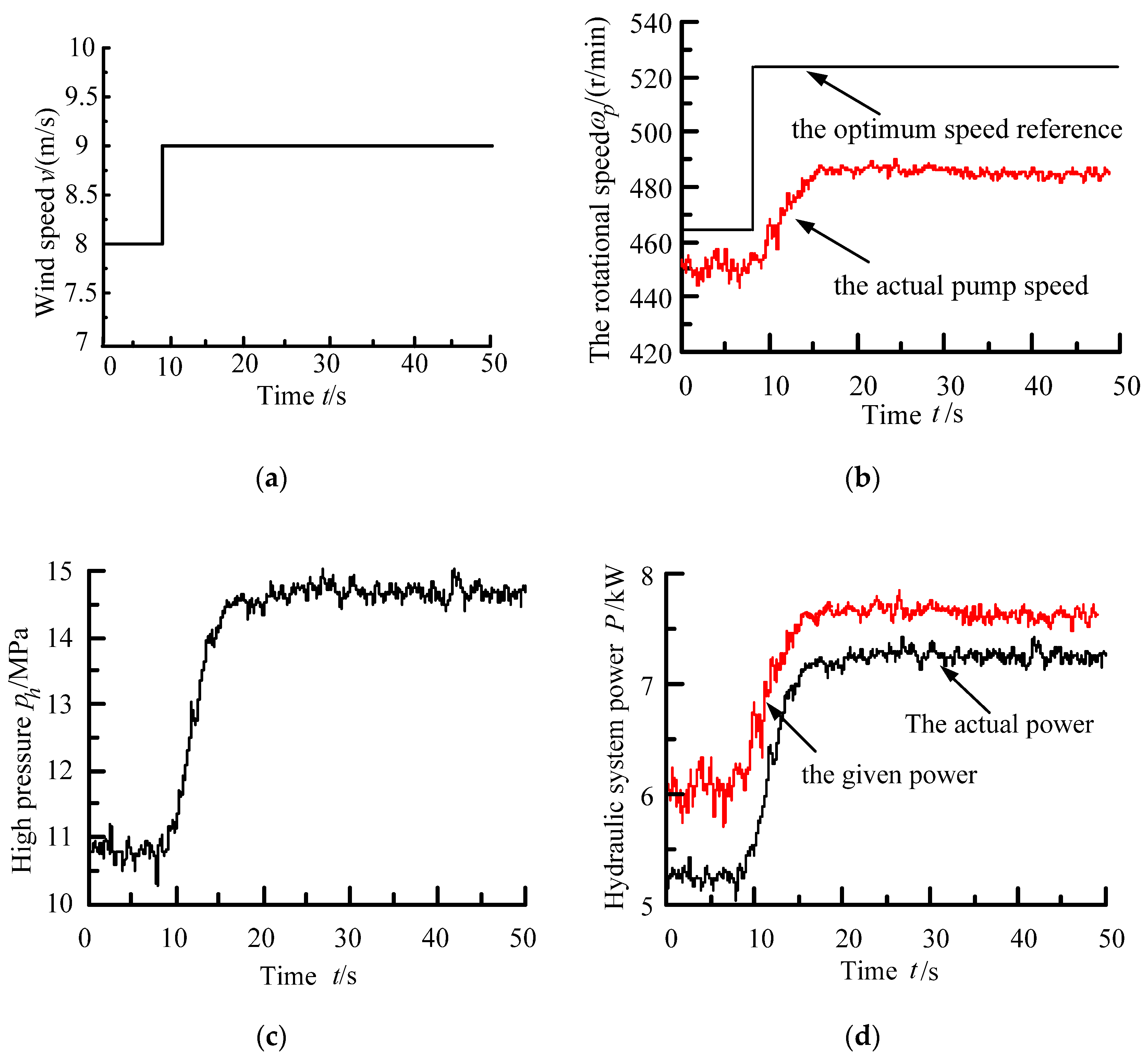
5.4. Experiment Analysis

Based on the above experimental platform and the pre-determined parameters, the MPPT control effect are researched under step wind speed of 8 m/s–9 m/s at 8 s, and the wind speed, the pump speed, system power, and high pressure are shown in Figure 10.
From Figure 10, through adjusting the motor displacement, the high pressure and pump speed change with step wind speed, the actual power also changes with the demand power. The response characteristics are basically the same as the simulation, and the system state changes stably under the step wind speed. However, there are differences between the demand power and actual power, and the reason is that the MPPT controller accuracy depends on the parameters.
The experimental parameters can be re-determined by experimental data. V / β can be obtained by the above experimental data. When the system is in a stable state, the dynamic change is equal to zero. Therefore, the acceleration term in the controller is 0, and the calculating formula for the motor swing angle can be expressed as
γ = D p ω p C t p h K m ω m d V β k 1 Δ P K m ω m d D p ω p
where v = d ( D p ω p p h ) / d t .
According to Formula (36), the controller contains three items, including the pump input flow, the leakage caused by the pressure and the oil-hydraulic contraction caused by the pressure. The first two items are the steady-state term, and the oil-hydraulic contraction caused by the pressure is the dynamic adjustment term. The HWT MPPT controller essentially converts power deviation into pressure change rate to dynamically adjust the motor displacement. The final steady-state term has a great influence on the system control. When the system reaches a stable state, the motor displacement should be the corresponding steady-state value related to the pump speed and the high pressure so that different power can be generated under each stable pump speed. Otherwise, repeated dynamic adjustments are needed to achieve stability. The pump displacement is a constant, so the leakage coefficient at different pump speed will ultimately affect the system stability. If the steady value is not accurate, it is easy to cause power generation instability by adjusting the dynamic term. Instead, the system will stabilize in other states. Therefore, it is difficult to guarantee the control accuracy in practical application, but the controller provides theoretical direction.

6. Conclusions

This paper takes the HWT as the research object; the state space model is established for HWT; hydraulic power is taken as the control output, and the MPPT control strategy for HWT is proposed based on the feedback linearization control method. The strategy effectively solves the power tracking control problem and strong nonlinearity problem, and the system smoothly and quickly tracks the demand power. The efficiency is about 83%, which mainly depends on the mechanical efficiency and volumetric efficiency of the HWT key hydraulic components. Although the output power tracks the demand power, it fluctuates greatly. The main reason is that the proposed controller depends on the model parameters and includes the leakage coefficient and other time-varying parameters, which leads to poor real-time performance of the controller. However, the proposed theoretical controller provides a reference for practical applications. Therefore, based on the engineering requirements, the control law is simplified and verified by experiments; that is, the output power can track the demand power accurately and smoothly.
The impact of uncertainty and strong time-varying parameters of the HWT MPPT control will be further studied later.

Author Contributions

Data curation, L.C.; formal analysis, Y.Z., J.G. and Z.H.; funding acquisition, C.A.; validation, Q.H.; writing—original draft, W.G.; writing—review and editing, H.Q. All authors have read and agreed to the published version of the manuscript.

Funding

This research was funded by National Natural Science Foundation of China grant number [51775476] and funded by the Excellent Youth Project of Hebei grant number [E2018203388].

Conflicts of Interest

The authors declare no conflict of interest.

Nomenclature

Variable SymbolVariable Specification
K P The optimal power coefficient, K P = ρ π R 5 C p max 2 λ o p t 3
P r max Maximum wind power absorbed by the rotor
ρ The air density
R The radius of a rotor blade
v The wind speed
C p max The maximum coefficient of wind energy utilize
ω r The wind turbine speed
λ o p t The optimum tip speed ratio
K P The maximum wind power coefficient
T p The pump torque
D p The pump displacement
p h The pressure difference between the pump suction and discharge lines
η m e c h , p The constant pump mechanical efficiency, which is assumed to be unity
T v ( ω p , v ) The rotor pneumatic torque
J p The pump moment of inertia
ω p The pump speed
B p The pump viscous damping coefficient
Q p The pump flow rate
C t 1 The pump leakage coefficient
T m The motor torque
D m The motor displacement
p h 2 The pressure difference between the motor suction and discharge lines
η m e c h , m The motor mechanical efficiency, which is assumed to be 1
K m The motor maximum displacement
γ The motor swing angle, ranging from 0 to 1
T L The motor load torque
Q b l The proportional flow valve flow rate
K The proportional coefficient
U E The voltage signal
Q c The flow rate caused by the oil compression.
V The pressure-affected oil volume
β e The effective oil bulk modulus including a correction for hose expansion
J m The motor moment of inertia
ω m The motor speed
B m The motor viscous damping coefficient
Q m The motor flow rate
C t 2 The motor leakage coefficient
Q c 1 The compressibility flow between the pump and the flow control valve
Q c 2 The compressibility flow between the motor and the flow control valve
x 1 The state variable 1
x 2 The state variable 2
ω md The demand motor speed
z 1 The state variable after coordinate transformation 1
z 2 The state variable after coordinate transformation 2
e The error
y d The system control input
y The system control output
v * The system controller
k 1 The control parameter 1
k 2 The control parameter 2

References

  1. Wei, J.; Sun, W.; Guo, A.; Wang, L. Analysis of wind turbine transmission system considering bearing clearance and thermo-mechanical coupling. In Proceedings of the World Non-Grid-Connected Wind Power Energy Conference, Nanjing, China, 24–26 September 2009; pp. 1–5. [Google Scholar]
  2. Liu, Z.G.; Yang, G.L.; Wei, L.J.; Yue, D. Variable speed and constant frequency control of hydraulic wind turbine with energy storage system. Adv. Mech. Eng. 2017, 9, 1–10. [Google Scholar] [CrossRef]
  3. Stelson, K.A. Saving the world’s energy with fluid power. In Proceedings of the 8th JFPS Int. Symp. Fluid Power, Okinawa, Japan, 25–28 October 2011; pp. 1–7. [Google Scholar]
  4. Jiang, Z.; Yang, L.; Gao, Z.; Moan, T. Numerical simulation of a wind turbine with a hydraulic transmission system. Energy Procedia. 2014, 53, 44–55. [Google Scholar] [CrossRef] [Green Version]
  5. Pedersen, N.H.; Johansen, P.; Andersen, T.O. Optimal control of a wind turbine with digital fluid power transmission. Nonlinear Dyn. 2018, 91, 591–607. [Google Scholar] [CrossRef]
  6. Yin, X.; Tong, X.; Zhao, X.; Karcanias, A. Maximum Power Generation Control of a Hybrid Wind Turbine Transmission System Based on H∞ Loop-Shaping Approach. IEEE Trans. Sustain. Energy 2019. [Google Scholar] [CrossRef] [Green Version]
  7. Ai, C.; Bai, W.; Zhang, T.; Kong, X. Research on the key problems of MPPT strategy based on active power control of hydraulic wind turbines. J. Renew. Sustain. Energy 2019, 11, 013301. [Google Scholar] [CrossRef]
  8. Yin, X.; Zhao, X. Sensor-less Maximum Power Extraction Control of a Hydrostatic Tidal Turbine Based on Adaptive Extreme Learning Machine. IEEE Trans. Sustain. Energy 2019, 11, 426–435. [Google Scholar] [CrossRef]
  9. Do, H.T.; Dang, T.D.; Truong, H.V.A.; Ahn, K.K. Maximum power point tracking and output power control on pressure coupling wind energy conversion system. IEEE Trans. Ind. Electron. 2018, 65, 1316–1324. [Google Scholar] [CrossRef]
  10. Farbood, M.; Sha-Sadeghi, M.; Izadian, A.; Niknam, T. Advanced Model Predictive MPPT and Frequency Regulation in Interconnected Wind Turbine Drivetrains. In Proceedings of the 2018 IEEE Energy Conversion Congress and Exposition (ECCE), IEEE, Portland, OR, USA, 23–27 September 2018; pp. 3658–3663. [Google Scholar]
  11. Li, S.; Shi, Y.; Li, J.; Cao, W. Maximum power point tracking control using combined predictive controller for a wind energy conversion system with permanent magnet synchronous generator. In Proceedings of the 2018 33rd Youth Academic Annual Conference of Chinese Association of Automation (YAC), IEEE, Nanjing, China, 18–20 May 2018; pp. 642–647. [Google Scholar]
  12. Mulders, S.P.; Diepeveen, N.F.B.; van Wingerden, J.W. Extremum Seeking Control for optimization of a feed-forward Pelton turbine speed controller in a fixed-displacement hydraulic wind turbine concept. J. Phys. Conf. Series. IOP Publ. 2019, 1222, 012015. [Google Scholar] [CrossRef]
  13. Deldar, M.; Izadian, A.; Anwar, S. A decentralized multivariable controller for hydrostatic wind turbine drivetrain. Asian J.Control. 2019. [Google Scholar] [CrossRef]
  14. Wang, F.; Chen, J.; Xu, B.; Stelson, K.A. Improving the reliability and energy production of large wind turbine with a digital hydrostatic drivetrain. Appl. Energy 2019, 251, 113309. [Google Scholar] [CrossRef]
  15. Ai, C.; Wu, C.; Zhao, F.; Kong, X. Optimal power tracking control of a hydraulic wind turbine based on the active disturbance rejection control. Trans. Can. Soc. Mech. Eng. 2019. [Google Scholar] [CrossRef]
  16. Akbari, R.; Izadian, A.; Weissbach, R. An Approach in Torque Control of Hydraulic Wind Turbine Powertrains. In Proceedings of the 2019 IEEE Energy Conversion Congress and Exposition (ECCE), IEEE, Baltimore, MD, USA, 29 September–3 October 2019; pp. 979–982. [Google Scholar]
  17. Wei, L.; Zhan, P.; Liu, Z.; Tao, Y.; Yue, D. Modeling and analysis of maximum power tracking of a 600 kw hydraulic energy storage wind turbine test rig. Processes 2019, 7, 706. [Google Scholar] [CrossRef] [Green Version]
  18. Alberto, I. Nonlinear Control Systems II; Athenaeum Press Ltd.: Gateshead, UK, 1999. [Google Scholar]
  19. Kong, X.D.; Ai, C.; Wang, J. A summary on the control system of hydrostatic drive train for wind turbines. Chin. Hydraul. Pneum. 2013, 1, 1–7. [Google Scholar]
  20. Ai, C.; Chen, L.J.; Kong, X.D. Characteristics simulation for hydraulic wind turbine. China Mach. Eng. 2015, 26, 1527–1531. [Google Scholar]
  21. Jiang, Z.H.; Yu, X.W. Modeling and control of an integrated wind power generation and energy storage system. In Proceedings of the Power Energy Soc. General Meeting, Calgary, AB, Canada, 26–30 July 2009; pp. 1–8. [Google Scholar]
  22. Wang, J.H. Advanced Nonlinear Control Theory and Its Application; Beijing Science Press: Beijing, China, 2012. [Google Scholar]
  23. Sreenath, K.; Park, H.W.; Poulakakis, I.; Grizzle, J.W. A compliant hybrid zero dynamics controller for stable, efficient and fast bipedal walking on MABEL. Int. J. Rob. Res. 2011, 30, 1170–1193. [Google Scholar] [CrossRef] [Green Version]
  24. Bharadwaj, S.; Rao, A.V.; Kenneth, D.M. Entry trajectory tracking law via feed-back linearization. J. Guid. Control Dyn. 1998, 21, 726–732. [Google Scholar] [CrossRef]
Figure 1. Schematic of the hydraulic wind turbine (HWT).
Energies 13 01529 g001
Figure 2. Schematic of the maximum power point tracking (MPPT) method for direct generation power control.
Energies 13 01529 g002
Figure 3. HWT MPPT control block diagram.
Energies 13 01529 g003
Figure 4. Feedback linearization control law flowchart.
Energies 13 01529 g004
Figure 5. Simulation model.
Energies 13 01529 g005
Figure 6. The response curve under the condition of 7 m/s-8 m/s step wind speed at 10 s. (a) the wind speed; (b) the pump speed; (c) the high pressure; (d) the output power.
Energies 13 01529 g006
Figure 7. the response curve under the condition of 8 m/s-7 m/s step wind speed at 10 s. (a) the wind speed; (b) the pump speed; (c) the high pressure; (d) the output power.
Energies 13 01529 g007
Figure 8. The response curve under 8 ± 0.5 m/s wind speed. (a) the wind speed; (b) the pump speed; (c) the high pressure; (d) the output power.
Energies 13 01529 g008
Figure 9. The structure diagram of 30 kVA semi-physical simulation platform.
Energies 13 01529 g009
Figure 10. The system response curve under the step wind speed. (a) the wind speed; (b) the pump speed; (c) the high pressure; (d) the output power.
Energies 13 01529 g010
Table 1. Control parameters.
NumberParameter SymbolValue
1 k 1 6
2 k 2 4
Table 2. Parameters of hydraulic drive system for experimental platform.
Parameter SymbolParameter NameValueUnit
B p the viscous damping coefficient of hydraulic pump0.4N.m.s/rad
D p the displacement of hydraulic pump1 × 10−5m3/rad
J p the inertia of hydraulic pump400kg/m3
K m the displacement gradient of variable displacement motor5.366 × 10−6m3/rad
B m the viscous damping coefficient of variable displacement motor0.0345N.m.s/rad
J m the inertia of hydraulic motor0.462kg/m3
β e the bulk modulus of hydraulic oil743 × 106Pa
C t the total leakage coefficient of hydraulic pump and variable displacement motor6.28 × 10−12m3/(s.Pa)
V the volume of oil affected by pressure effect in hydraulic hose2.8 × 10−3m3
P the output power of wind turbine24kW
Rradius of wind turbine7.48m
C p max the maximum coefficient of wind energy utilized0.4496
λ max the optimal tip speed ratio22.77
Table 3. 24 kW semi physical simulation experiment platform components.
Serial NumberNameModel
1variable frequency motoryvp250m-4
2speed torque sensorjn338a
3hydraulic fixed displacement pumpa2f63r2p3
4pressure sensorzq-bz-1/hk/m20
5pressure gaugeyn-63-i-31.5
6relief valvedb10a-1-b30/315
7check valves20p1.0b
8accumulatorsb330-10a1/112a9-330a
9variable displacement motora4vso40ds1/10w-ppb13t013z
10excitation synchronous generatorwf200-24
11vane pumppfe-41085
12relief valveagm20-a-20/100y
13relief valveagm20-a-20/315y
14constant pressure variable pump63pcy14-1b
15relief valvedbds10g10b/25/2
16air coolerok-el5s/3.1/m/a/1

