Article

Pre-Drilling Production Forecasting of Parent and Child Wells Using a 2-Segment Decline Curve Analysis (DCA) Method Based on an Analytical Flow-Cell Model Scaled by a Single Type Well

Harold Vance Department of Petroleum Engineering, Texas A&M University, 3116 TAMU College Station, TX 77843-3116, USA
*
Author to whom correspondence should be addressed.
Energies 2020, 13(6), 1525; https://doi.org/10.3390/en13061525
Submission received: 8 February 2020 / Revised: 3 March 2020 / Accepted: 17 March 2020 / Published: 24 March 2020

Abstract

:
This paper advances a practical tool for production forecasting, using a 2-segment Decline Curve Analysis (DCA) method, based on an analytical flow-cell model for multi-stage fractured shale wells. The flow-cell model uses a type well and can forecast the production rate and estimated ultimate recovery (EUR) of newly planned wells, accounting for changes in completion design (fracture spacing, height, half-length), total well length, and well spacing. The basic equations for the flow-cell model have been derived in two earlier papers, the first one dedicated to well forecasts with fracture down-spacing, the second one to well performance forecasts when inter-well spacing changes (and for wells drilled at different times, to account for parent-child well interaction). The present paper provides a practical workflow, introduces correction parameters to account for acreage quality and fracture treatment quality. Further adjustments to the flow-cell model based 2-segment DCA method are made after history matching field data and numerical reservoir simulations, which indicate that terminal decline is not exponential (b = 0) but hyperbolic (with 0 < b< 1). The timing for the onset of boundary dominated flow was also better constrained, using inputs from a reservoir simulator. The new 2-segment DCA method is applied to real field data from the Eagle Ford Formation. Among the major insights of our analyses are: (1) fracture down-spacing does not increase the long-term EUR, and (2) fracture down-spacing of real wells does not result in the rate increases predicted by either the flow-cell model based 2-segment DCA (or its matching reservoir simulations) with the assumed perfect fractures in the down-spaced well models. Our conclusion is that real wells with down-spaced fracture clusters, involving up to 5000 perforations, are unlikely to develop successful hydraulic fractures from each cluster. The fracture treatment quality factor (TQF) or failure rate (1-TQF) can be estimated by comparing the actual well performance with the well forecast based on the ideal well model (albeit flow-cell model or reservoir model, both history-matched on the type curve).

1. Introduction

Hydrocarbon well development in shale leases commonly occurs at a very high pace, because the return on capital invested in the lease region needs to be maximized to meet investor expectations. The operator of a shale lease may be assumed to have acquired the acreage with the expectation to make a profit. The typical modus operandi to achieve that goal in US leases is to drill all wells parallel to the lease boundary, with the tightest possible well spacing, and complete each of the wells with hydraulically-fractured stages that move from toe to heel in laterals of two miles long (~10,000 ft long horizontal section of the well) in less than two weeks.
The technical prowess of a company is often touted as the distinguishing factor. However, in shale operations, the basic technology is now well-established (e.g., see collated papers in [1]). Field development strategies generally are based on the assessment of a fairly limited number of key aspects: (1) Where in the lease region occur the highest hydrocarbon in place volumes? (2) What is the optimum well spacing? (3) What is the optimum fracture spacing in each well? (4) What fracture treatment program can achieve the desired facture spacing with infinite conductivity over much of the fracture half-length? (5) What is the best production lift system?
A vast body of practical operational experience has been established (mostly in the US, China, and Argentina) over the past two decades in unconventional oil and gas fields that have been developed with an astonishing number of wells (>100,000). For the operators, the uncertainties that may affect their return on investment reside in externalities (e.g., oil and gas prices volatility) and in internalities (e.g., original hydrocarbons in place and recovery factors). Combined with analyses of the gathered data and history matching the hydraulic fracture development models with actual pump rates, and history matching of production performance against reservoir models, industry has progressively refined their estimations of the key reservoir parameters and improved well completion techniques to boost the recovery factors.
In spite of all the advances made by the oil and gas industry, recovery factors in shale fields remain low and returns on investment are marginal or lacking at concurrent oil and gas prices, which has resulted in hundreds of bankruptcies [2]. What shale operators need to do is optimize field development by selecting the richest lease regions for drilling and using optimized fracture spacing and well spacing. Reservoir models of hydraulically fractured wells have been notoriously cumbersome to use in hydraulically fractured reservoirs, due to gridding issues and inability to model discrete fractures without introducing oversized grid cells with enhanced permeability. A fairly large number of independent shale operators have no reservoir modeling units and entirely rely on empirical well performance improvements, guided mostly by well performance forecasts and estimated ultimate recovery (EUR) estimations based on decline curve analysis (DCA) methods [3]. Although DCA methods are very practical for history-matched forecasts of existing wells [4,5], such traditional DCA methods cannot predict the performance of wells that have not yet been drilled and for which no historic data is available, especially when completion parameters, fracture spacing, and well spacing of the new wells have no direct analogy to the prior wells.
Recent work in our research group has paved the way for accurate pre-drilling DCA-based well performance forecasts based on an analytical flow-cell model [6,7]. The flow-cell based 2-segment DCA uses a type well to scale the production performance of newly planned wells, with the distinctive capacity to fully factor in the effects of changes in well length, fracture spacing, fracture height, fracture half-length, and variable well spacing. In short, the 2-segment DCA based on the analytical flow cell model can be claimed to provide the same accuracy, but is much faster and easier to use, than a gridded reservoir model. EUR estimates given in the present study and comparison of flow-cell based forecasts with those from commercial reservoir simulators confirm this claim (this study).
The present study advances the flow-cell based 2-segment DCA method further with benchmark wells, enhances the accuracy of estimations for the onset of boundary dominate flow, and adjusts the terminal decline curve from exponential to hyperbolic, based on calibration with field data and with numerical reservoir simulations using commercial simulators (CMG and KAPPA). Further, a practical workflow is given for use of the 2-segment DCA spreadsheet (based on flow-cell model calibrated with a type curve) for production forecasting of parent and child wells. Application of the new method to various thoroughly investigated wells from the Eagle Ford Formation (Brazos Valley) have revealed many nuances and practical insights, the implications of which are highlighted in the present study.

2. Contemporary Research and New Direction

This section first places our research in concurrent context (Section 2.1) and then proceeds to explain our new flow-cell based DCA method (Section 2.2). Moreover, a practical workflow (Section 2.3), typical inputs needed, and outputs generated (Section 2.4) are also outlined.

2.1. Brief Review of Practical Tools for Well Performance Prediction

Well performance prediction in unconventional shale plays has been a subject of substantial research interest, and still is a rapidly evolving study topic. For example, a wide range of history matching methods with decline curves has been proposed. Single-segment DCA algorithms include Power Law Exponential Decline [8,9], Stretched Exponential Production Decline [10], Duong’s (2011) model [11], and the Logistic Growth Model [12]. Additional post-Arps DCA methods have been proposed by Patzek et al. [13], Zhang et al. [14], de Holanda et al. [15], and Miao et al. [16]. Since almost all of the proposed alternatives to Arps have their own limitations, the quest for improved, practical DCA methods continues [5,17].
When the cost of US shale acreage rose from the $25-$100/acre range in early 2000 to $10,000–$50,000/acre over the past decade, optimum use of acre space became more important for operators. Detailed workflows have been designed to help shale operators make decisions about optimum well spacing and completion design [18,19,20,21,22]. Operators are particularly concerned about the adverse impacts on well productivity when well spacing is reduced. For example, operators in the Midland Basin (West Texas) use well spacing between 400 and 1400 ft, and no consensus exists about what is the optimum spacing. The principal gains may come from extending the effective fracture half-length, such that fewer wells need to be drilled [23]. Efforts to optimize the fracture length have to weigh the considerable uncertainty about the effective permeability of the reservoir region that the fractures need to drain [24]. If the reservoir space is comprised of 25 nD rock permeability, then the hydraulic fractures need to be much longer (>500 ft) to drain the same production as in a 850 nD reservoir with short fractures (~100 ft). Obviously, the well solution with shorter fractures would require development with a denser spacing of the laterals.
Early field development used larger well spacing, which led operators to later infill drilling with so-called child wells [21]. The impact of the interaction of parent and child wells and risk of inter-well communication via fracture hits of wells placed to closely is also an area of detailed research [25,26,27,28,29,30]. In addition to physics-based models [31], many operators resort to data analytics to find the optimum well spacing and completion parameters based on historic data sets. Such data-driven searches for multivariate correlations have no primary objective to understand the physics of the processes involved, but simply search for completion parameters that the best performing wells have in common [29]. Although such correlations are useful, they also preclude forward learning, because data-driven searches remain confined to the past performance of the wells in the data set. When physics-based insights lead to innovation in well development, data analytics quickly loses touch with reality, because data from the leading edge wells are sparse and would barely weigh in the correlations based on past performance [23].
Although many operators tend to seek clues in big data and data analytics, the impression that such approaches are capable of solving all problems may be overblown [32]. The main reasons listed for failure to fulfill the expectation include (1) data-driven methods are not designed to model the structural characteristics of the underlying system, (2) ’blind’ big data projects have no conceptual guidance from the physical processes involved, and (3) if the past physics-based solutions for field development were inadequate, data-driven solutions cannot be better than the underlying data. What is sieved out in the multivariate correlations is the underperformers, no more, no less.

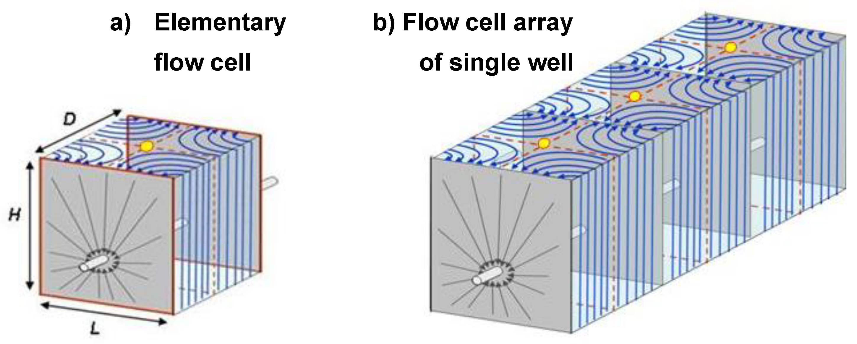
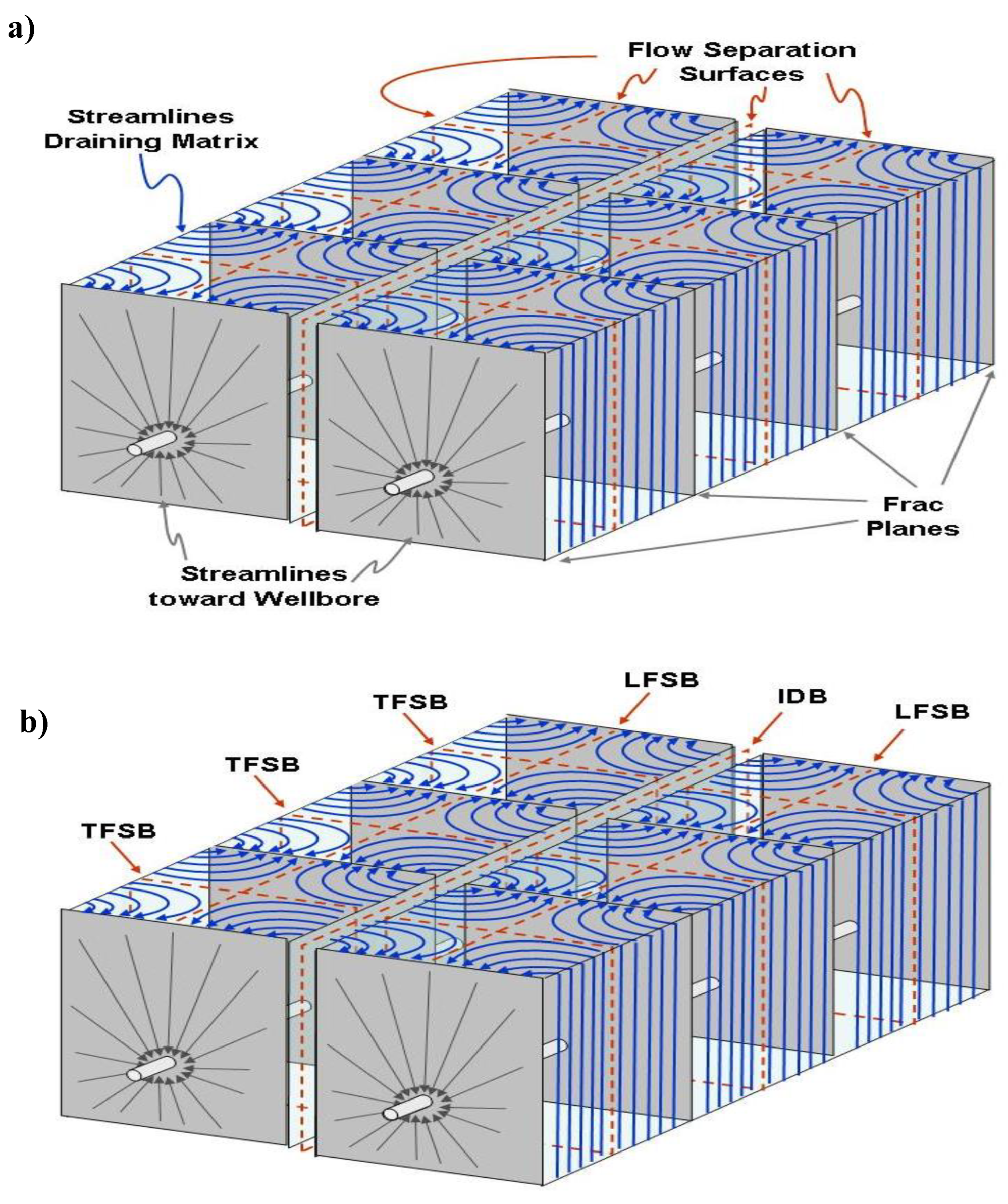
2.2. Basic Flow-Cell Model Description

The flow-cell based 2-segment DCA spreadsheet model is grounded in a comprehensive set of recently derived analytical expressions that quantify well interference due to competition for flow space between the hydraulic fractures in parent and child wells and also between parent-parent well pairs. The concept of an elementary flow-cell model was introduced for the specific purpose of creating a solution method of reductionist nature that can be implemented in a practical spreadsheet and account for the impact of well interference. The analytical expressions and key equations and parameters used are based on Complex Analysis Methods (CAM) that can provide solutions for fluid flow paths, velocity distribution, time-of-flight contours, and reservoir depletion patterns. The majority of the detailed derivations and benchmarking of results can be found in two prior publications [6,7].
The flow-cell model based on CAM solves for the flow interaction between multiple fractures based on material balance principles. Solutions for the basic flow cells can be constructed for individual flow cells confined between hydraulic fracture surfaces in a single well (Figure 1a,b). An important recognition of the flow-cell model is the definition of various flow space boundaries within a single well and also between multiple wells (Figure 2a,b).
The basic flow-cell model assumes single-phase flow. The onset of well interference is determined from computing when the pressure transient of the well has reached the interwell drainage boundary (IDB) using the theoretical depth of investigation formula (Equation (1)). The radius of investigation (ri) refers to the advance of the pressure drawdown front, which expands from the well outward. The transient radius of investigation, ri, at time t, varies with the reservoir properties (porosity, ϕ ( z ) and permeability, k ( z ) , fluid viscosity, μ, and compressibility, ct):
r i ( t ) = k ( z ) t 1688.7 ϕ ( z ) μ c t           [ ft ]
The time corresponding to the ‘discovery’ of a nearby well, marking the advent of True Boundary Dominated Flow (BDF), is given by (equating ri=distance to IDB):
t = r i 2 ( t ) 1688.7 ϕ ( z ) μ c t k ( z )           [ s ]
The timing of the onset of True BDF will vary with well spacing (distance to IDB) and the onset of BDF affects the decline of type curve wells input into the spreadsheet. All of these analytical expressions and concepts are incorporated into the Excel-spreadsheet to account for well interference effects on daily production rates and estimated ultimate recovery (EUR) forecasts for unconventional reservoirs.

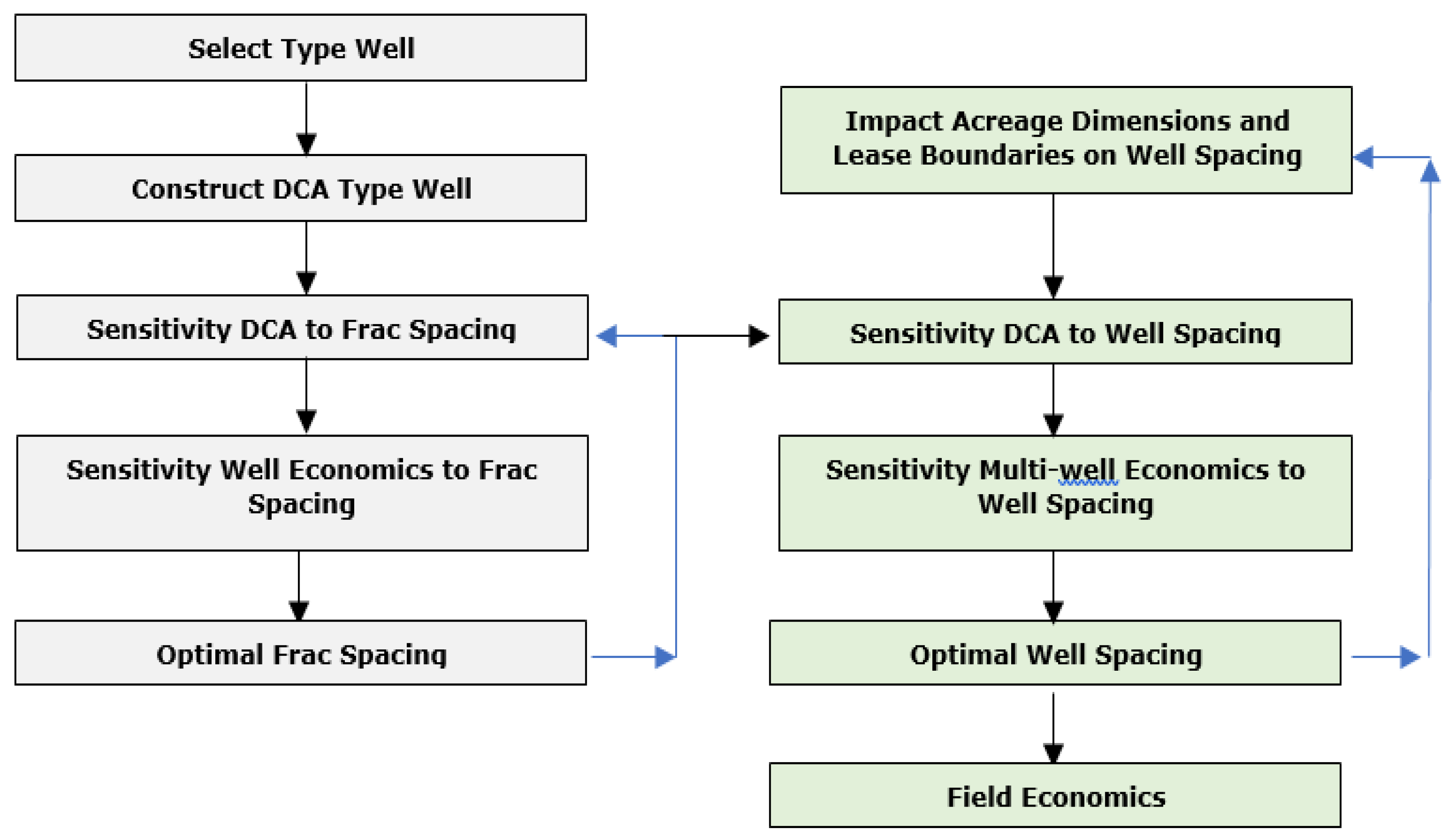
2.3. Practical Workflow Steps

The purpose of this study is to further explain the function and broad application potential of the new analytical flow-cell model developed to forecast with a 2-segment DCA method the impact of hydraulic fracture down-spacing and well interference in unconventional reservoirs. The well interference comes about due to changes in well spacing between adjacent horizontal hydraulically fractured wells in ultra-low permeability shale reservoirs. Differences in well spacing will realize different timings for the onset of the boundary dominated flow regime, which herald terminal decline and result in accelerated well productivity decline.
The left column in Figure 3 focuses first on fracture spacing optimization of newly planned wells. The starting point is a type well constructed based on a legacy well with known completion parameters and at least 36 months production data to allow for the construction of a reliable type curve. The "solver" method used for determining the DCA parameter of qi, b, and Di is briefly explained in Appendix A.
Once the DCA parameters for the type curve well have been identified, the next step is to explore the effect on well productivity of fracture down-spacing. The flow cell formulation can account for any changes to fracture spacing in the new wells, as well as changes in fracture half-length, height, and overall well length. Daily and cumulative production plots are automatically generated. The fracture spacing should be optimized based on the evaluation of production data with a cash flow-analysis module. Once the optimum fracture spacing has been established, the next step is well-spacing optimization (Figure 3, right column).
In addition to completion parameter changes (fracture spacing, height and half-length), the 2-segment DCA model can account for well spacing changes for both simultaneous parent-parent wells as for parent-child wells (with a time delay of their respective drilling and completion). Based on the predicted performance of the parent and child wells, the production forecast of the lease region can be optimized using again a standard cash flow analysis.

2.4. Required Model Inputs and Outputs Generated

A more accurate capturing of the terminal decline rates and the proper timing of their onset will result in better decline forecasts for both daily production values as well as for cumulative produced volumes. The 2-segment DCA method based on the analytical flow-cell model provides a fast tool to effectively capture the effects on well productivity of changes in fracture treatment design and well spacing changes. Quantifying the impact of the associated well interference effects in a practical 2-segment DCA spreadsheet results in fast and reliable production forecasts that allow for quick calculations of economic viability of the possible different well configurations and fracture treatment design parameters in unconventional reservoirs. Comparison of practical EUR estimations for Eagle Ford wells with the new 2-segment DCA method, with prior estimates based on independent methods, shows reliable results are attained.
A brief interface guide to the flow-cell based 2-segment DCA method is given in Appendix A. The inputs needed for the spreadsheet and the outputs produced to be used by the engineer for further economic and commercial analysis are explained below.
-
Inputs required:
  • production data of type curve well (to scale the flow-cell rate),
  • estimated reservoir properties (to control the rate of the pressure transient),
  • dimensions of elementary flow-cell of the type curve well (against which the new well with different flow-cell dimensions will be scaled),
  • total well length (to account for changes relative to the type well length),
  • well spacing for the type curve well (to account for well down-spacing effects),
  • acreage quality factor (to account for any changes in well performance due to geological factors, if applicable, separate from the well design and completion impacts).
-
Outputs produced:
  • future production rates and EUR of new wells,
  • forecasts possible for parent–parent wells,
  • forecasts possible for parent–child wells,
  • fracture treatment quality (FTQ) factor, which shows the quality difference between planned completion (design) and practical completion (actual results).

3. Flow-Cell Model Results: Fracture Spacing Effects

Application of CMG and KAPPA simulators, and comparison with the flow-cell based DCA models, to real world examples has revealed a number of valuable insights about the imperfections that occur in well completion operations, in particular about the quality of hydraulic fracture treatment jobs. The fracture treatment imperfections came to light as follows. Firstly, the general adequacy of the flow cell-based well performance forecasts due to fracture down-spacing was demonstrated in our two prior papers [6,7].
The type well curve used in our prior study was from Well H1 in an Eagle Ford lease located in Brazos Valley [5,33]. Meanwhile, we have enough historic production data available from two later wells (H2 and H3). The two new wells were landed in the same bench (Wells H2 and H3), which is why we confidently assume an acreage quality factor (AQF) of 1; no change in well performance is expected based on geological factors. The well completion details are given in Table 1. We next started out history matching the Eagle Ford type well (H1) and the new wells (H2 and H3) using various methods.
- Acreage quality factor (AQF): Although operators tend to select drilling locations with the highest original hydrocarbon in place (OHIP) volumes, major differences in OHIP may occur due to regional variations in reservoir quality. High quality acreage sections were historically located by geological exploration, involving petrophysical assessment of organic maturity, and estimated volumes of hydrocarbons in place. With the dense number of wells available in all major US shale plays, and a fairly uniform completion practices at any moment in time, the spatial variations in average well performance for a basin or formation can be abstracted using data analytics. In our flow-cell model, if needed, the acreage quality of the type well region can be translated to an acreage quality factor by normalizing the new well EUR with the EUR of the type well. The resulting fraction is the AQF and can be used to adjust the expected production rate of a new well based on the type well. For example, the typical 24-month EUR for an Eagle Ford well in Brazos County is 83k barrels (bbls), while in LaSalle County it is 103k bbls, which gives for Brazos County referenced to LaSalle County an AQF = 0.8 and for LaSalle referenced to Brazos County AQF = 1.25 (assuming the type curve well is located in the County used for EUR normalization). Other adjustments due to technical well design changes can be accounted for based on the physics-based input parameters in the flow-cell model (see later in this section).

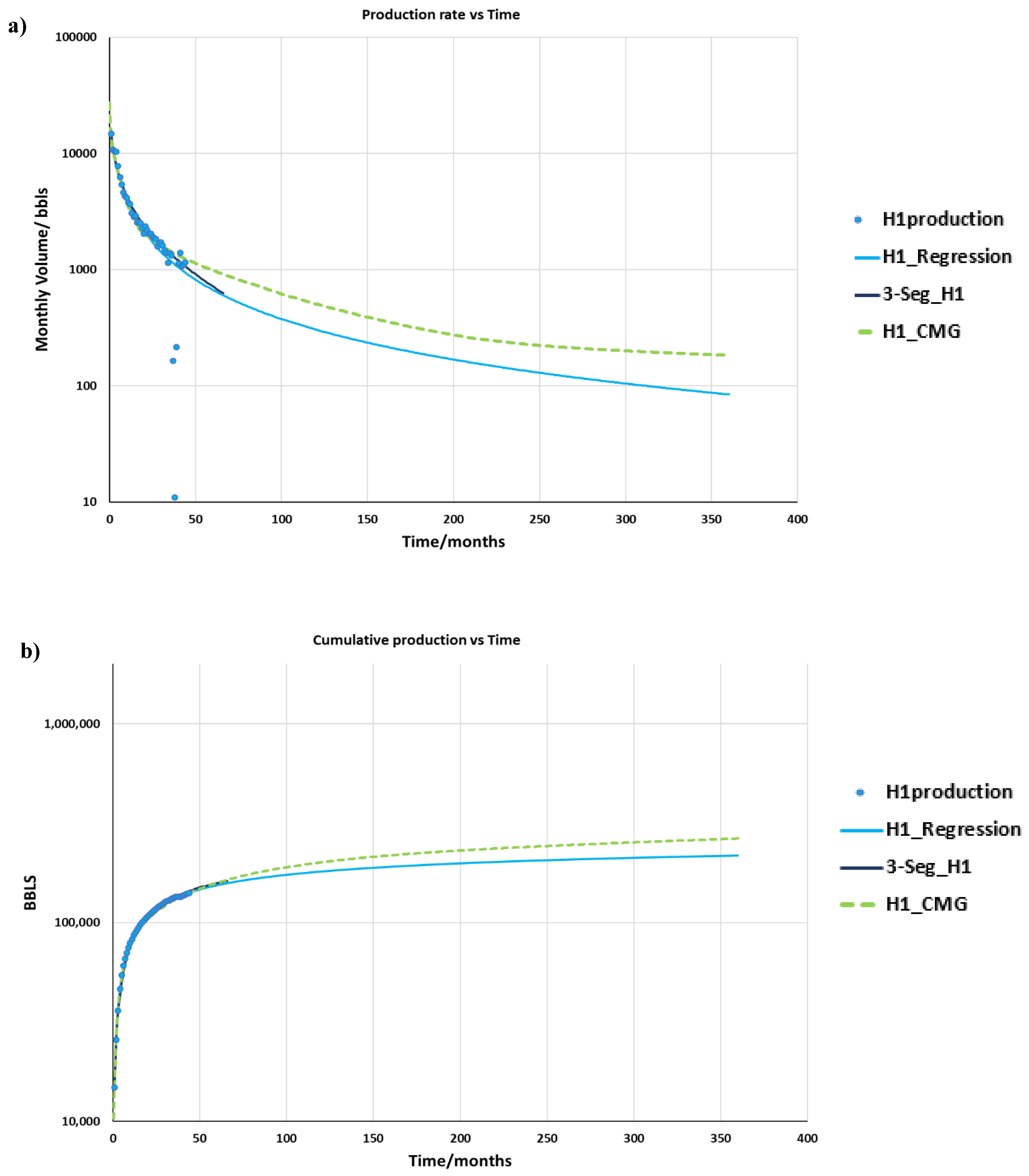
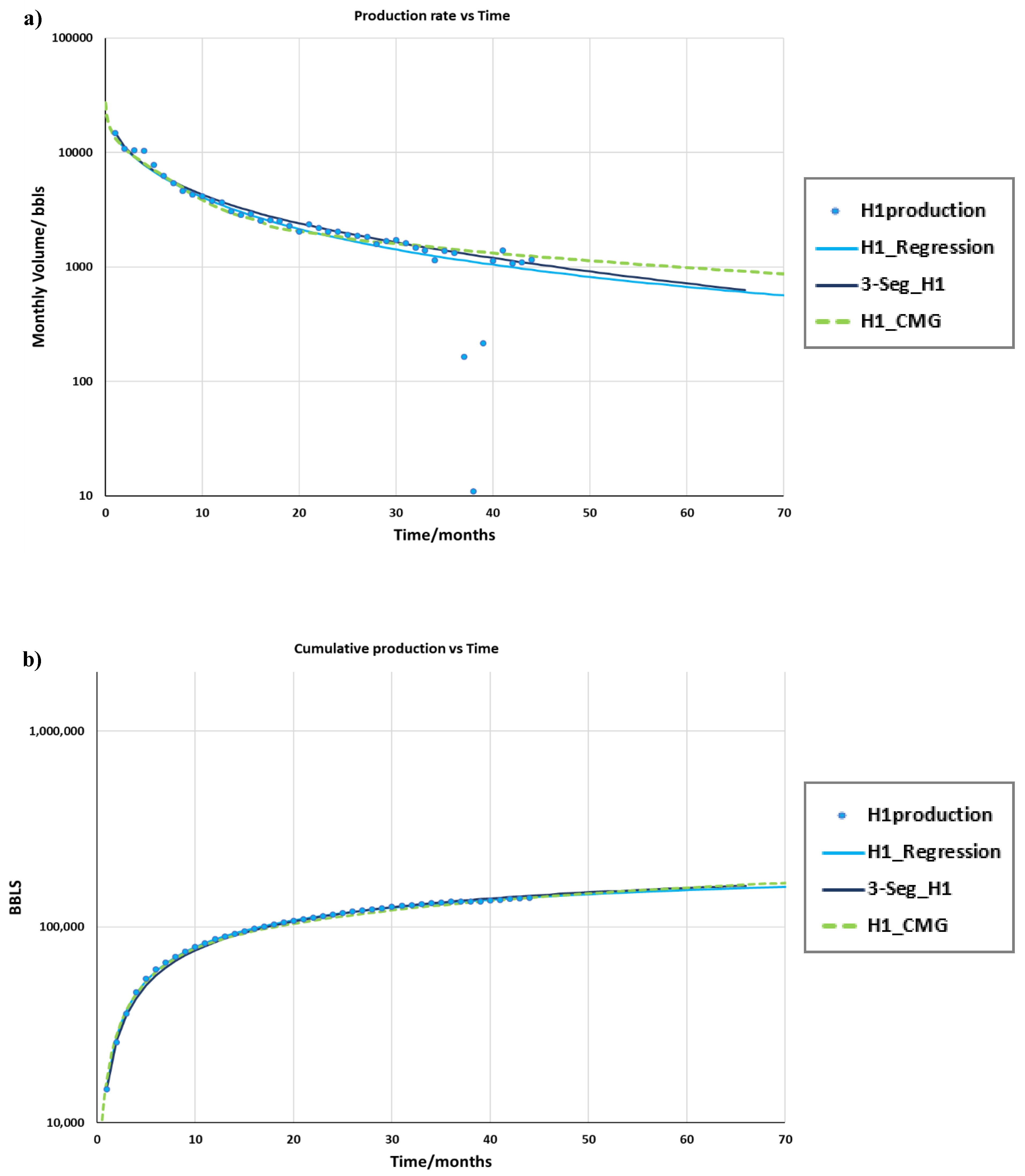
3.1. History Matching Type Well and Reservoir Simulator

In a first step of the workflow (see Section 2.3), the H1 type well DCA curve is generated by history matching historical production data. Such a history match was performed here using three methods: (1) a single Arps (1945) DCA fit [34], (2) a more advanced 3-segment DCA fit [5], and (3) a CMG history match (Figure 4). The CMG Well H1 history match was discussed in detail in two prior studies [35,36]. The 3-segment DCA of Well H1 was subject of two separate in-depth studies [5,17].
The variation in the history matched type curves (Figure 4a,b) is evident. The CMG history match for Well H1 (dashed) results in higher estimates for the long-term well performance, as compared to the two DCA regression-based production rate and EUR forecasts in Figure 4a,b. The simple DCA history match can best be used as a basis for the 2-segment DCA models for new wells. The 3-segment DCA would be more cumbersome to use, because the type curve would be comprised of three distinct segments.
When we look closer at the various history matches for the economically important first five years (60 months) of production (Figure 5a,b), then the reservoir model-based CMG history match is still satisfactory. The simple DCA history match was further used in the flow-cell based 2-segment DCA forecast of new wells, but CMG forecasts of type well H1 and a later Well H3 were also used for comparison with the 2-segment DCA forecasts.

3.2. EUR Forecasts and History Match Comparisons New Wells

We next provide the flow-cell based 2-segment DCA production rate forecasts for wells H2 and H3, together with a CMG-based forecast for well H3 (Figure 6), using the fracture down-spacing parameters of Table 1. The CMG history match model parameters have been given in a prior study [35]. In addition, in Figure 6, are the actual production data for Wells H2 and H3 (giving 6-months and 17-months DCA regressions for each well, see Figure legend for more detail), augmented with 3-segment DCA fits for Wells H1, H2, and H3 from a recent study [5]. The benchmark of Figure 6 clearly shows that DCA regression based on 6 months production data (Wells H2 and H3) is unreliable and vastly overestimates the actual well performance when looking at the cumulative produced volume.
In addition, the long-term EUR is matched by the flow-cell based DCA curves for H2 and H3, as well as by the CMG curve for Well H3. Closer inspection of early time performance (Figure 7), reveals that actual well performance (simple DCA and 3-segment DCA) is matched less well by either of the forecast models (e.g., both the CMG and flow-cell models overestimate early well rates).
The zoomed image of Figure 7 highlights that the H2 and H3 actual well performance does not comply with the CMG and flow-cell based model forecasts. The well spacing of the Wells H2 and H3 was identical to that of the parent well H1 and all wells tapped into the reservoir sections with same original oil in place volumes. The production gains of fracture down-spacing evidently are less than expected based on the well models with down-spaced fractures. A poor performance of child wells is often attributed to well interference effects. While this certainly may play a role in some regions, our well simulations (flow-cell based and CMG) invariably suggest that failed perforations and fracture coalescence into several principal hydraulic fracture swarms is the principal cause of a relatively lagging production performance. Introduction of a fracture treatment quality factor (TQF) in the flow-cell based model leads to very close matches of the actual Well H2 and H3 performance (see Section 3.5).

3.3. Decline Rate Forecasts New Wells

The corresponding production rate forecasts for the new Wells (H2 and H3), according to the various methods, are compiled in Figure 8 and Figure 9, for respectively the long-term (30-year) and short-term (5-year) time scales. We consider the simple DCA curve based on history matching 17 months of historic production data for Wells H2 and H3 as the actual well performance. The 6-month DCA regression curves are considered unreliable.
Both Wells H2 and H3 seem to have slightly higher rates than the flow-cell based long-term forecasts (Figure 8). However, Figure 9 shows that early in the well life the flow-cell based forecast for Wells H2 and H3 give well rates higher than for Well H1 (as was expected based on wider fracture spacing for the latter), but also is initially higher than the actual H2 and H3 performance.
Again, the zoomed image of Figure 9 highlights that Wells H2 and H3 actual 17 months DCA performance does neither comply with the CMG nor the flow-cell based model forecasts. The well spacing of the Wells H2 and H3 was identical to that of the parent well H1 and all wells tapped into the reservoir sections with same original oil in place volumes. The production gains of fracture down-spacing evidently are less than expected based on the well models with down-spaced fractures. However, introduction of a fracture treatment quality factor (TQF) in the flow-cell based model leads to very close matches of the actual Well H2 and H3 performance (Figure 10a,b; only H2 shown for brevity).

3.4. Fracture Treatment Quality Factor (TQF)

A key aspect of the flow-cell model is the possibility to adjust the flow cell size according to the intended fracture spacing as controlled by the perforation cluster spacing used during completion of the hydraulic fracture treatment of the isolated fracturing stages. However, creating the required fractures as planned is still a challenging task, involving numerous technical decisions. For example, which hydraulic fracturing fluid composition is best and at what rate and for how long should it be pumped into the stages? How much and at what rate should proppant load (and what mesh distribution) be pumped? The flow-cell model does directly factor in the required fracture dimensions (spacing, height, and half-length), but not the fracture treatment parameters.
By comparing actual well performance with predicted performance (Section 3.3), it is possible to determine what fraction of the fractures in the actual well was completed successfully, which is captured in a fracture treatment quality factor (TQF) that expresses which percentage of the intended fracture surface is contributing to the well rate. Figure 10a,b show that the flow-cell based forecast of Well H2 can be made to match the actual well performance when reducing the number of active hydraulic fractures.
The principal reasons for the disparity between planned fracture dimensions and actual hydraulic fractures created are numerous: failed perforations, poor stage isolation, behind casing migration of fracturing fluid, merging of fractures of closely spaced perforation clusters into densely spaced fracture swarms, failure to establish effectively propped fracture half-length. All these factors for a given well jointly consolidate in the fracture treatment quality factor (TQF). When TQF = 1, the fracture spacing is as planned. When TQF < 1, the fraction says which percentage of fractures has failed, or did not establish the planned fracture half-length. When TQF > 1, the fraction indicates that the net product of successful fractures times and the effectively propped half-length times fracture height has outperformed the planned overall surface area of the hydraulic fractures.

3.5. Comparison of Flow-Cell Based EUR and Numerical EUR Estimation Methods

An overview of the 30-year EUR estimations with the various method is given in Table 2:
  • simple Arp’s hyperbolic using 6 months production data seems to vastly overestimate EUR for H2 and H3 (Figure 6, Figure 7, Figure 8 and Figure 9);
  • 3-segment DCA may have more accurate EUR but this requires historical data for each well; more data more accuracy (Figure 6, Figure 7, Figure 8 and Figure 9 and Table 2);
  • the flow cell model (scaling of decline parameters) that takes H1 as the type curve gives higher EUR than the 3-segment DCA for H2 and H3 (Table 2);
  • assumptions of all flow cells having same fracture length and aperture may not hold which leads to flow-cell model over-predicting EUR when TQF is not included (Figure 10a,b and Table 2);
  • inclusion of TQF shows flow-cell model matches 2-Segment DCA (Figure 10a,b).

4. Flow-Cell Model Results: Well Spacing Effects

The flow-cell based forecast for well down-spacing were tested using benchmark data provided by a commercial three-dimensional (3D) numerical reservoir simulator (Figure 11, Rubis module of KAPPA Workstation v.5.12.06) to generate production curves for an initial type well and show the impact of well spacing reduction. A reduction in well spacing was simulated by setting the formation boundary equal to the distance to the Inter-well Drainage Boundary (IDB), given by the half-well spacing (ye). The input parameters used in the model have been described in detail in work by Tugan and Weijermars [5] and Weijermars et al. [7]. The new well to type well spacing ratio (W/TW) is given by the new well spacing (W) divided by the original spacing of the type well (TW).

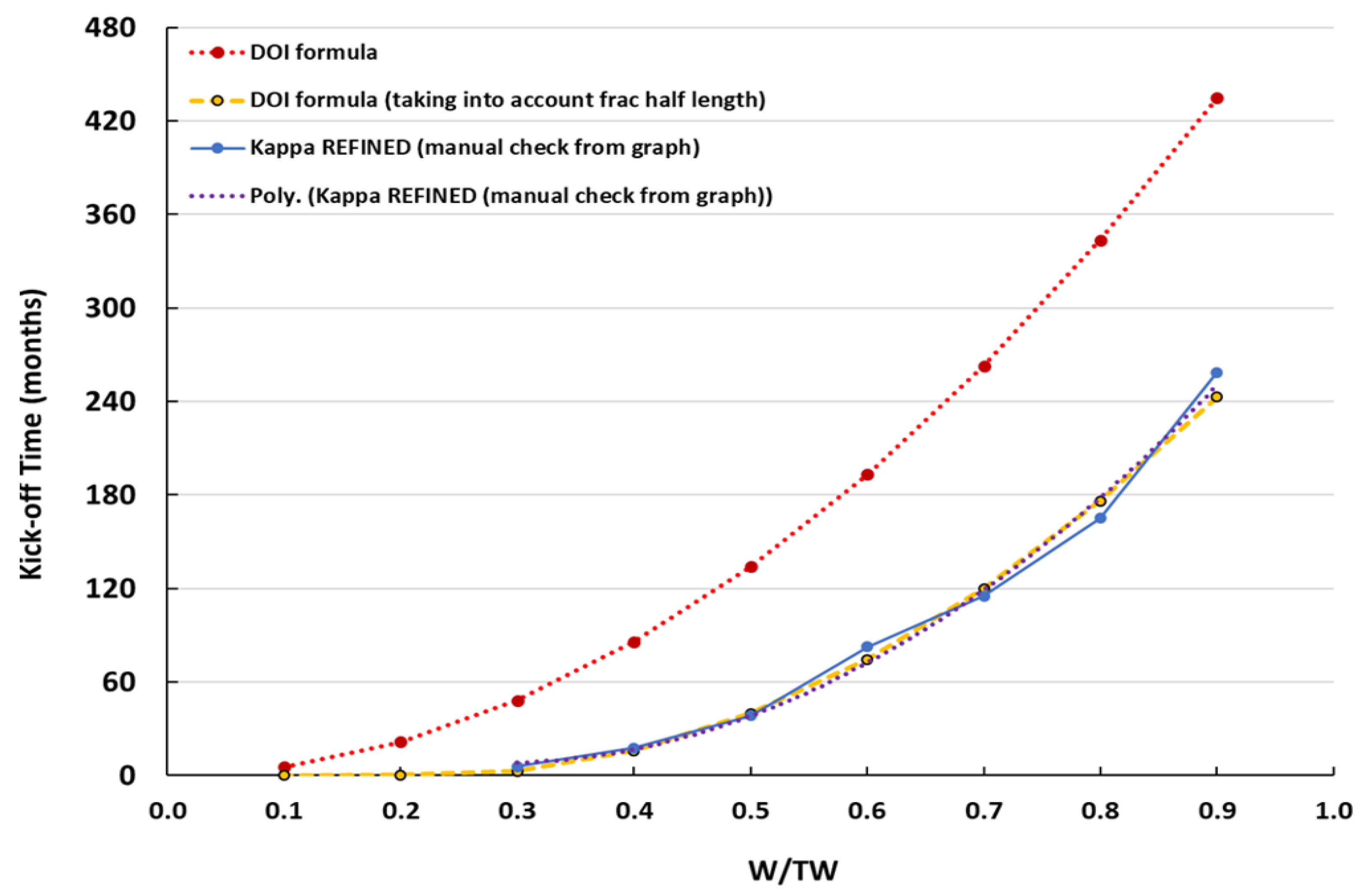
4.1. Onset of Terminal Decline

Figure 12a plots the daily and cumulative production data, based on the KAPPA-Rubis model, for a range of inter-well spacings. For higher well spacing, the flow behavior remains nearly the same as for the history matched type well H1. For example, the 11-year (4000 days) EUR difference for well spacing ratio (well to type well ratio) W/TW = 1.0 and W/TW = 0.7 is only a few thousand barrels at the end of 30-year well life (Figure 12b). However, for a further reduction of well spacing (W/TW < 0.7), the drop in EUR becomes progressively more severe because the daily flow rates of the tighter spaced wells are affected much earlier by well interference early in the well life. For example, for W/TW = 0.6, the EUR reduces significantly as compared to W/TW = 0.7.
Careful inspection of Figure 12b reveals that the reduced well spacing leads to rapid decline in the well rate when the kick-off points herald the onset of terminal decline. We already noted in our earlier study [7] that the terminal decline in the KAPPA model of Figure 12b is not exponential, counter to what was assumed in the original flow cell model.
Based on the KAPPA model results, two corrections to the flow-based model were required. The first correction concerned the timing of the kick-off points in the KAPPA model curves, which occurred earlier than in the flow-cell based model, which initially assumed the pressure transient to start propagating from the wellbore. Careful comparison of KAPPA kick-off times with those from the original flow-cell based model quickly revealed that the simple depth of investigation (DOI) formula (Equation (1)) given previously, leads to a near perfect match with KAPPA kick-off times, provided the pressure transient is computed to start from the fracture tips (Figure 13). Table 3 gives the corresponding time at which the kick-off points are reached when the well spacing is reduced.

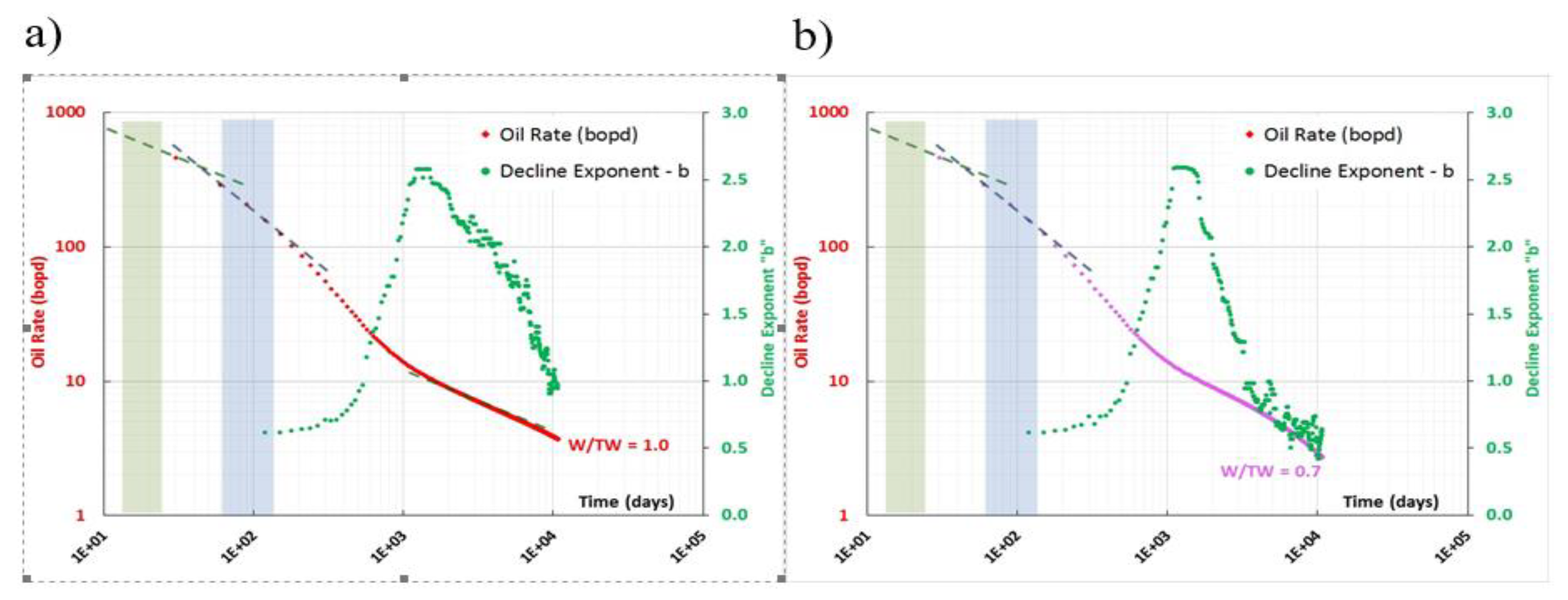
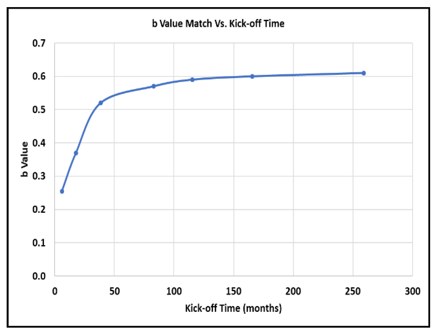
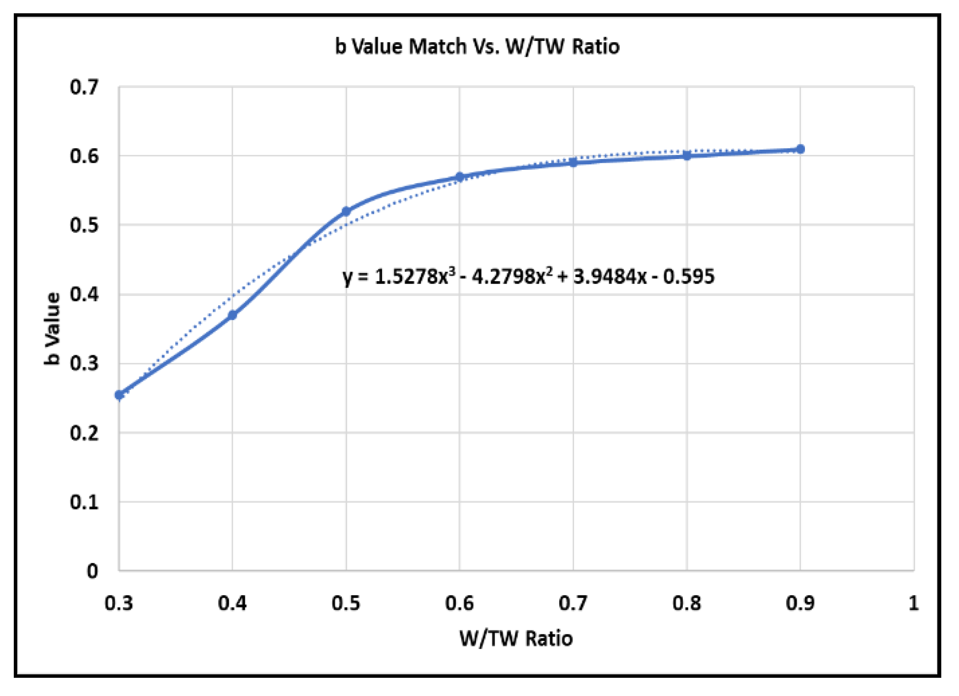
4.2. Terminal Decline and b-Values

The second correction in the flow-cell based 2-segment DCA was that the terminal decline in the KAPPA models with the tighter well spacing was clearly not exponential, but resembled a hyperbolic trend (Figure 12b). We history matched the KAPPA b-values versus kick-off time (Table 4) and used those b-values for the second DCA segment in the flow-cell model (Figure 14a,b). The updated flow-cell based forecast of well-spacing reduction of Figure 14a,b matches very closely with the KAPPA forecast of Figure 12a,b). A limiting exponential decline rate [37] is clearly too idealistic, because the Transverse Flow Separation Boundaries (TFSB) (see Figure 3b) provides partial boundary dominated flow long before the adjacent well is discovered.

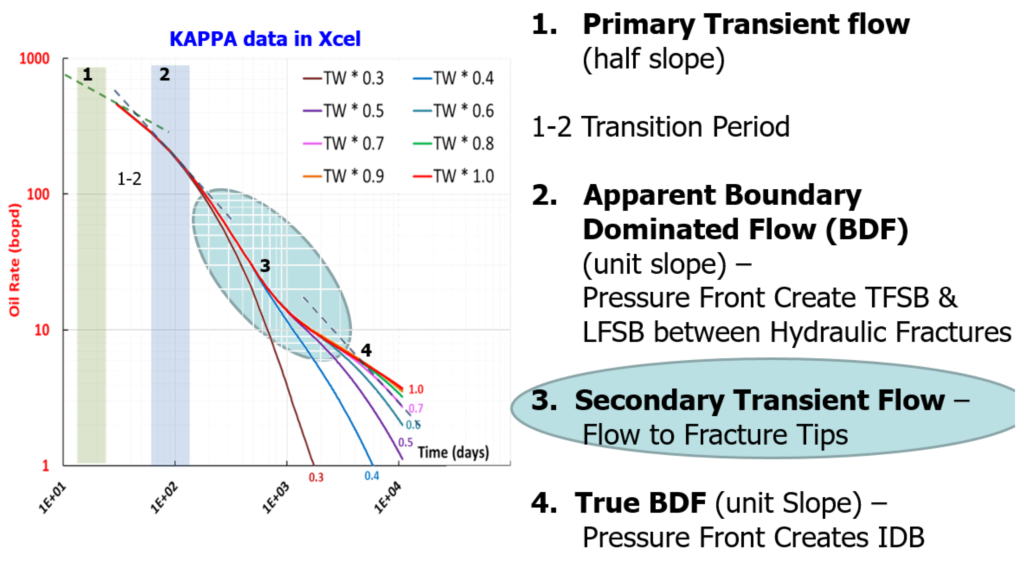
4.3. Terminal Decline and Flow Regime Changes

Analysis of the flow regime changes (Figure 15) confirms that terminal decline is not occurring in a True BDF regime, but rather in Secondary Transient Flow. Consequently, the terminal decline of with the tighter well spacing is not exponential, but resembles a hyperbolic trend.

4.4. B-Sigmoid Confirmation of Terminal Decline With 1 > b > 0

The analysis of b-sigmoid patterns based on instantaneous b-values (Figure 16) for the analyzed well spacing of W/TW of 1 shows the late-life b-values converge on 1, and for narrower well spacings (e.g., W/TW = 0.7) decreases further to b = 0.5. These results are congruent with a terminal decline still being hyperbolic decline (with 0 < b < 1) rather than exponential (b = 0).

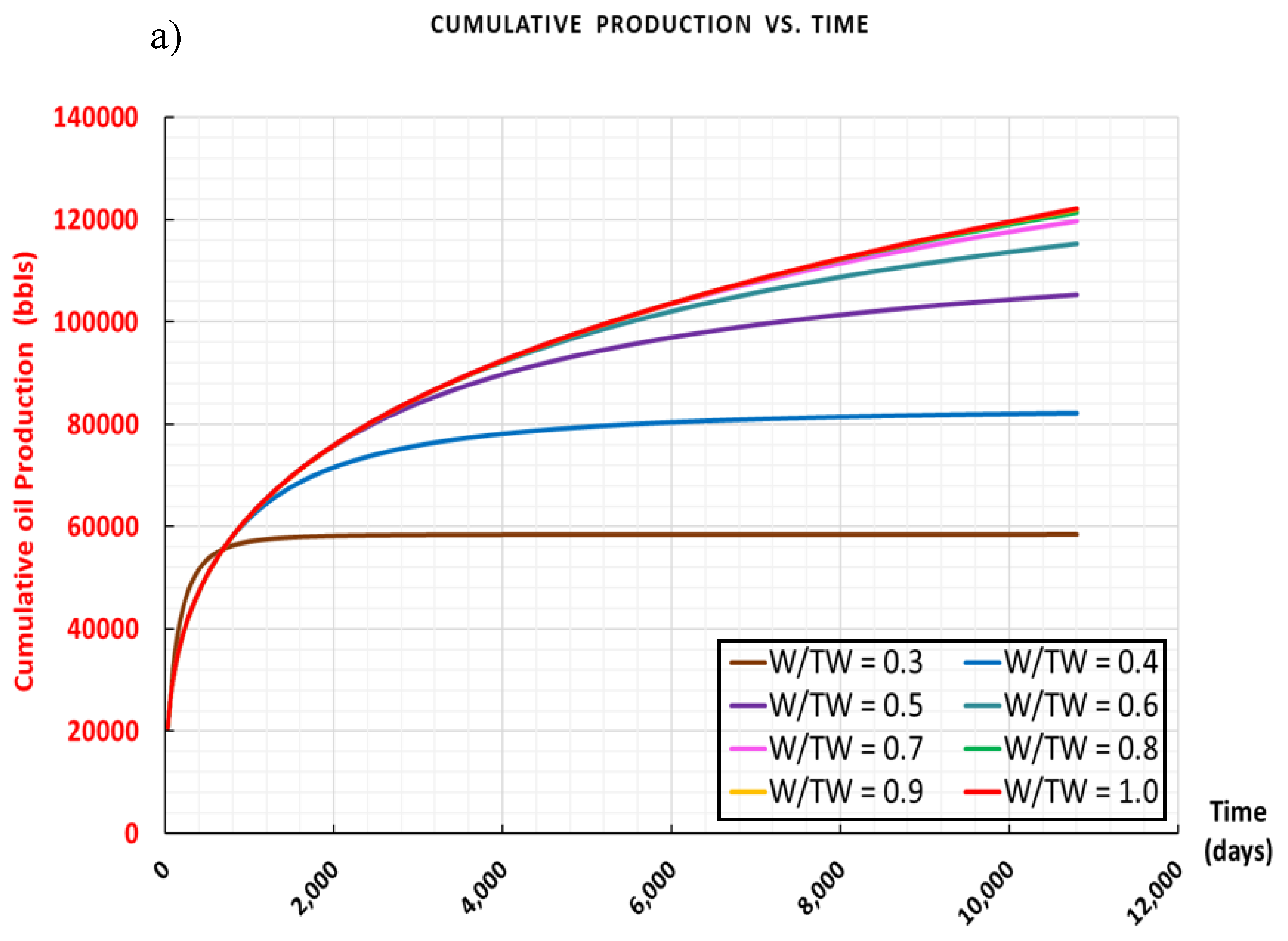
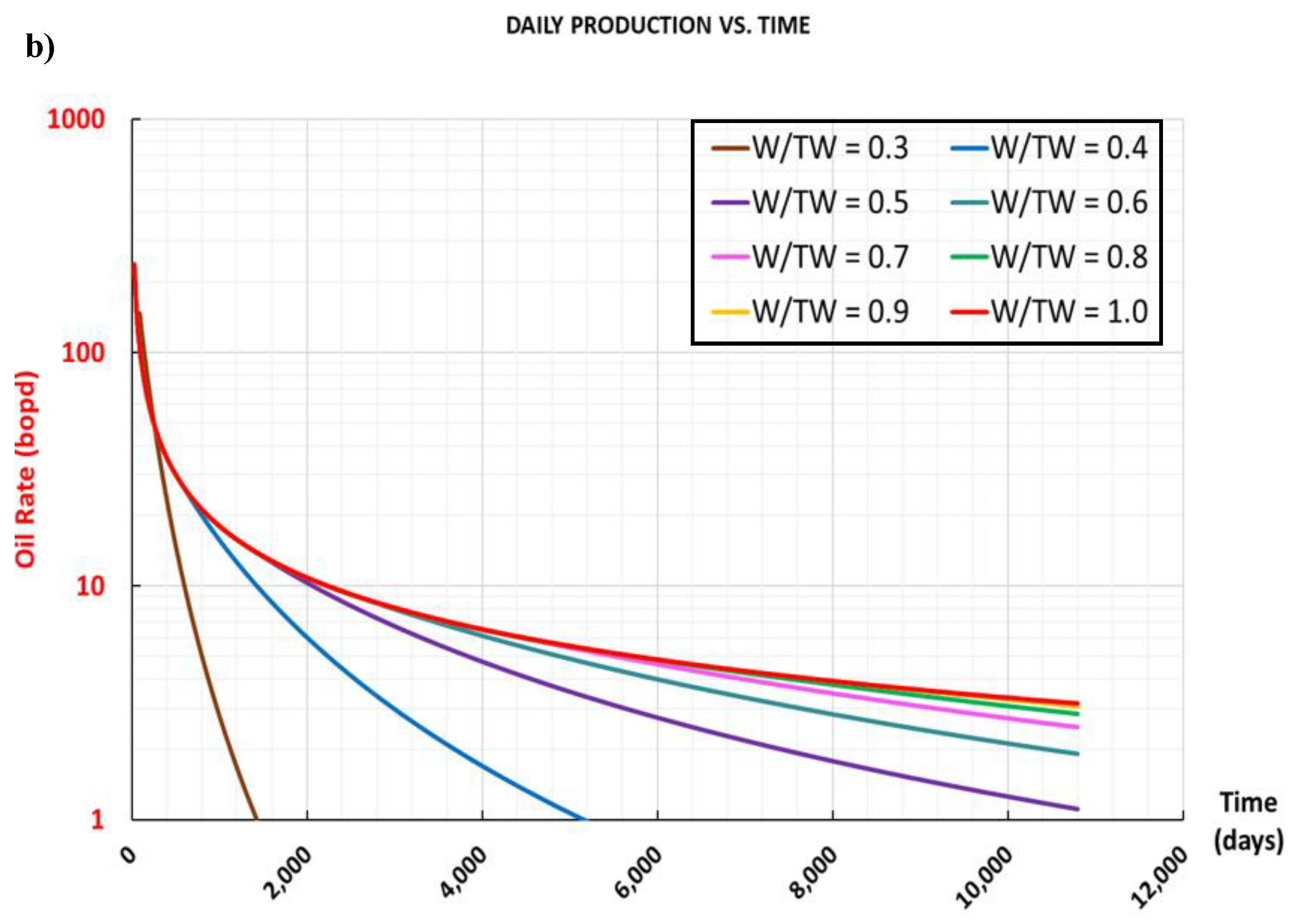
4.5. Comparison of Flow-Cell Based EUR With KAPPA Results

A final confirmation of the validity of the newly developed flow-cell model with the inclusion of the secondary hyperbolic decline is demonstrated by a comparison of EUR values (Table 5). The EURs computed from the flow-cell model-based 2-segment DCA are compared to those from the original KAPPA model. The flow-cell model determines the ‘kick-off points’ by use of the DOI formula, now assuming the pressure transient starts from the hydraulic fracture tips. The secondary hyperbolic decline b-value used in the flow-cell model is obtained from the history match of the KAPPA model decline. The EUR-values presented in Table 5 for the various decreasing well spacing show that, for 30-year EUR forecasts, the difference between the KAPPA numerical simulation model and the flow-cell analytical solution is never more than 4%. This difference in EUR is comparable with the differences of various forecasting methods. Among the practical advantages of the presented flow-cell model are its speed, affordability, simplicity, and ease of use.

5. Discussion

The present paper advocates the use of practical spreadsheet-based production forecasting model accounting for the acreage quality from data analytics that is commercially available, using a type curve from a representative parent well with certain known completion parameters (e.g., fracture half-length, height and spacing, and well spacing).

5.1. Generic Observations

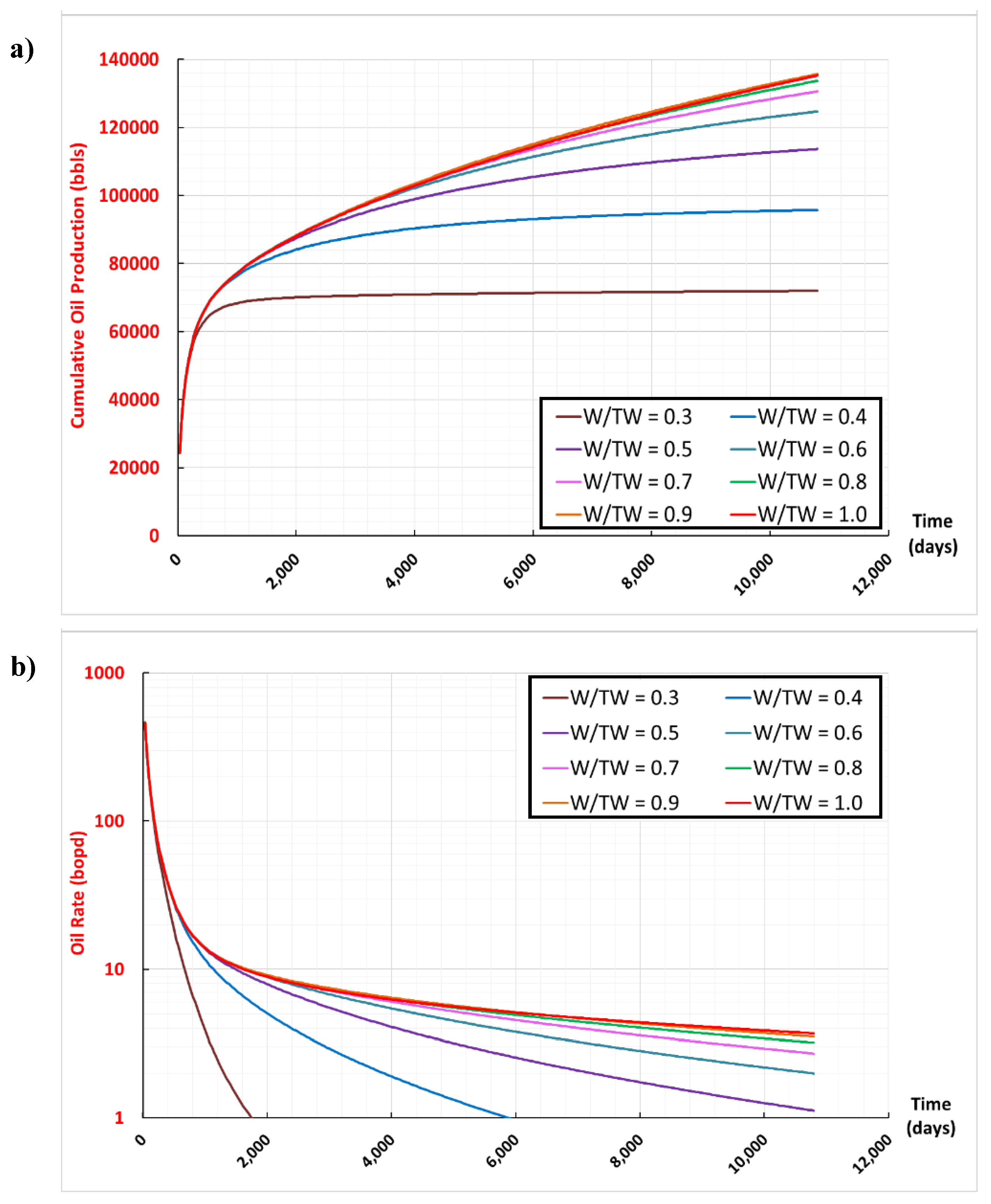
  • Recovery factors are not noticeably enhanced by fracture treatment with tighter fracture spacing, assuming that well interference effects due to well down-spacing remain negligible. Only early production rates are higher at the expense of late-well life production rate. Pressure depletion will occur faster in the zones between hydraulic fractures when fracture spacing is reduced, which initially leads to higher production rates, but lower production rates thereafter, due to rapid depletion of pressure such that flow rate of the well declines accordingly.
  • When tighter fracture spacing is used, the likelihood of poorly performing perforation clusters increases. Two child wells studied underperformed relative to the predicted CMG and KAPPA reservoir model forecasts. The well spacing of the child wells was identical to that of the parent wells and all wells tapped into the reservoir sections with same original oil in place volumes. The production gains of fracture down-spacing are less than expected. A poor performance of child wells is often attributed to well interference effects. While this certainly may play a role in some regions, our well simulations suggest the possibility of failed perforations and fracture coalescence into several principal hydraulic fracture swarms is the principal cause of relatively lagging production performance.
  • In any case, tighter fracture spacing, although not leading to overall EUR gains (computed here for the typical 30-year time frame), is still of interest to operators because some early production gains are booked, which benefits the internal rate of return of the project (due to time value of money used in discounting the project cash flows). Each year over the past 15 years, service providers have innovated by providing competitively priced completion packages with more fracture stages and tighter fracture cluster spacing. That is what service providers of completion technology compete on and industry seems each year to adopt the tightest perforation cluster spacing possible in their newly completed wells. The common perforation cluster spacing used in North America becomes tighter each year.
  • Well rates, when reaching the boundary dominated flow regime, do not decline exponentially, as has been often assumed in two segment DCA models. The exponential decline model is over-simplistic as the transition from secondary transient flow to true BDF occurs gradually, due to which a terminal rate with hyperbolic decline is more appropriate, as was demonstrated in our study by history matching the flow-cell model against a KAPPA reservoir simulation.
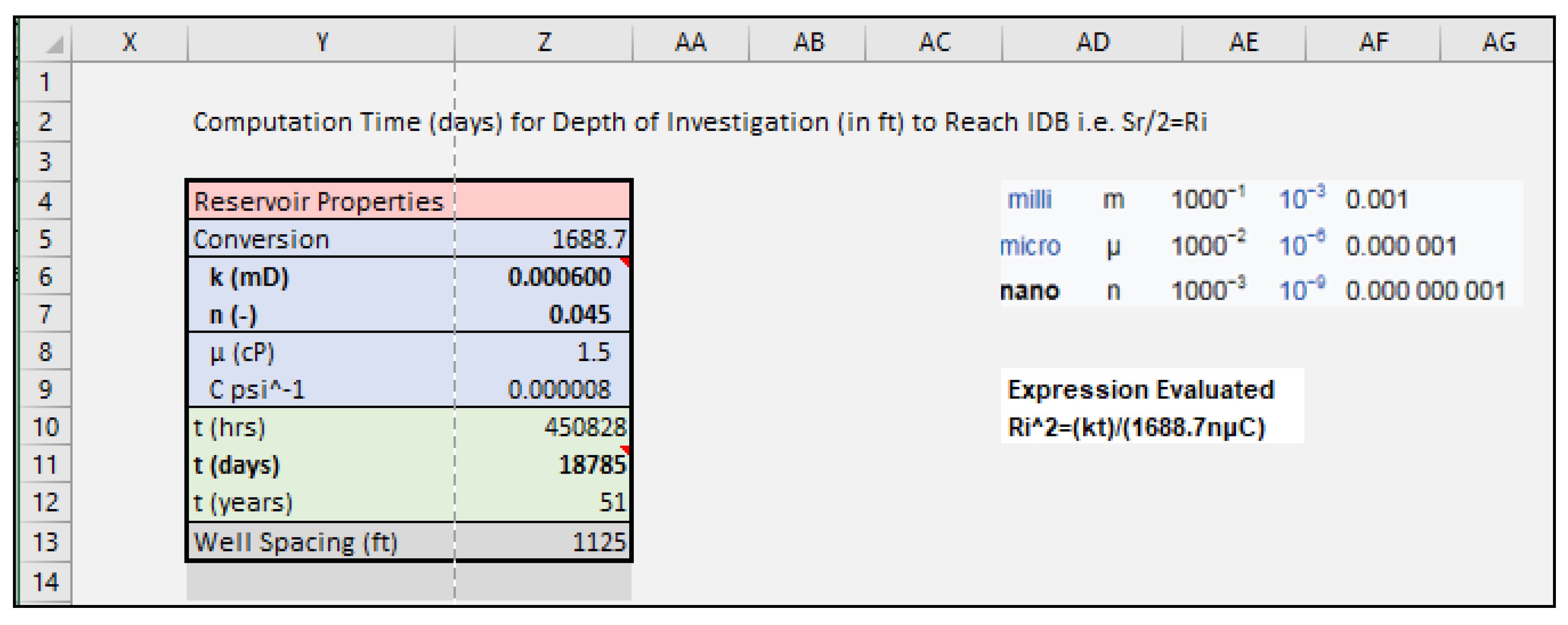
  • The onset of true BDF, or kick-off points on the type curve can be approximated by a depth of investigation curve, but more accurate results are achieved by calibration of the timing of kick-off using a reservoir simulator. Once the curve for kick-off timing is established, the flow-cell model will give reasonably accurate production forecasts for well spacing reduction.
  • Long wells cannot be argued to suffer from pressure bottlenecks in productivity due to frictional flow losses in the hydraulic fractures system and the production system. Such frictional losses are not the limiting factor, which entirely resides in the sluggishness of diffusion of reservoir fluids in the nano-Darcy reservoir space.
  • Different reservoir simulators give different history matches for the flow performance of hydraulically fractured wells, and only converge in production forecasts when mutually exclusive reservoir parameters are used. Our example used CMG and KAPPA simulators. The flow-cell model based on the type curve combined with reservoir model-based kick-off points provides a fast, practical alternative, with plausible accuracy.
  • Bubble point effects are not (yet) accounted for. Equation of state computations would need be integrated with the spreadsheet model (work in progress).

5.2. Additional Insights From Models

  • Future performance and history matching results are greatly dependent on fluid and PVT model as relative permeability curves will affect late-life well rates in a profound way. Bubble point effects may lead locally to rapid pressure decline but lift up the well rate later due to its gas lift effect.
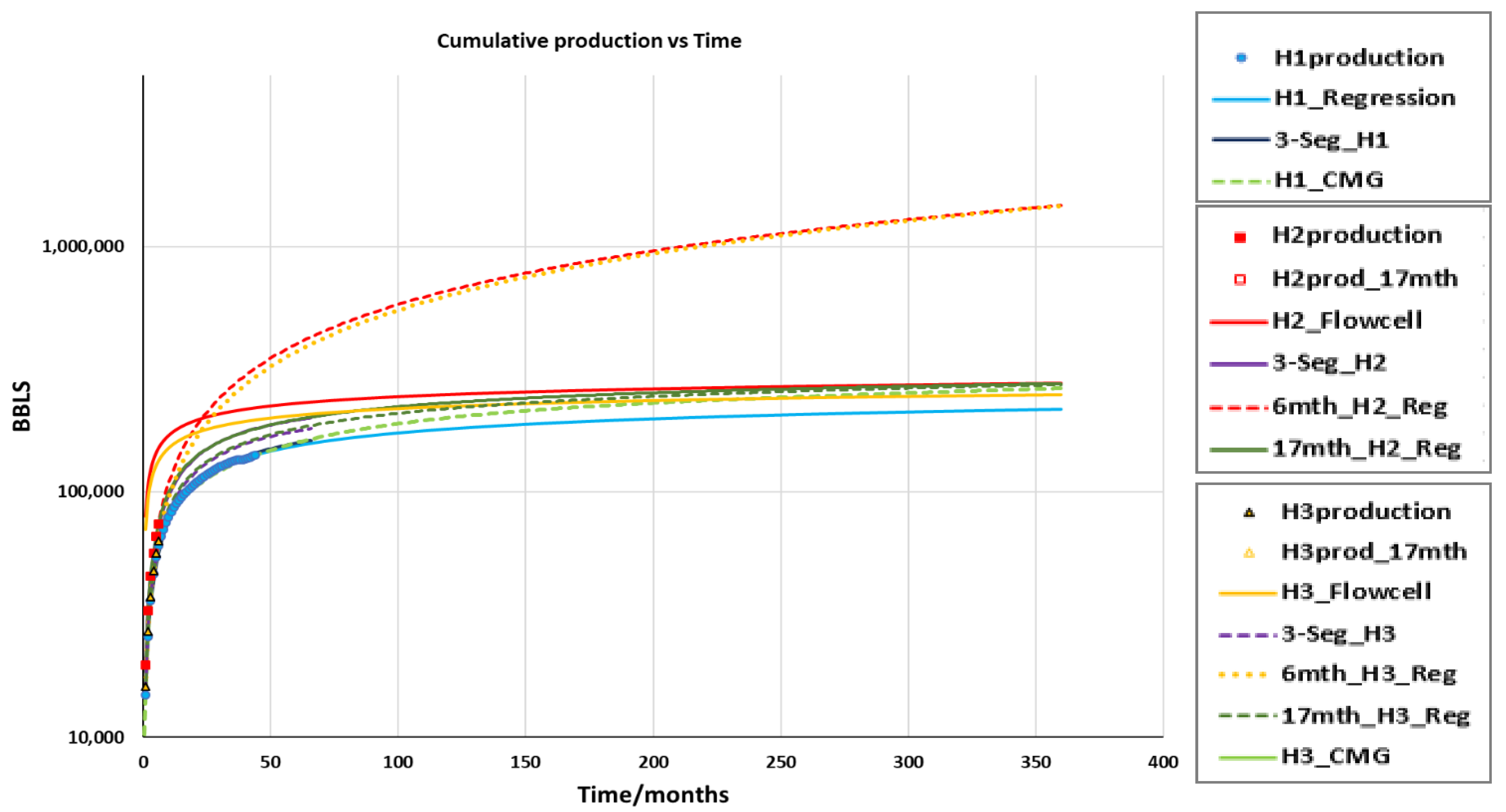
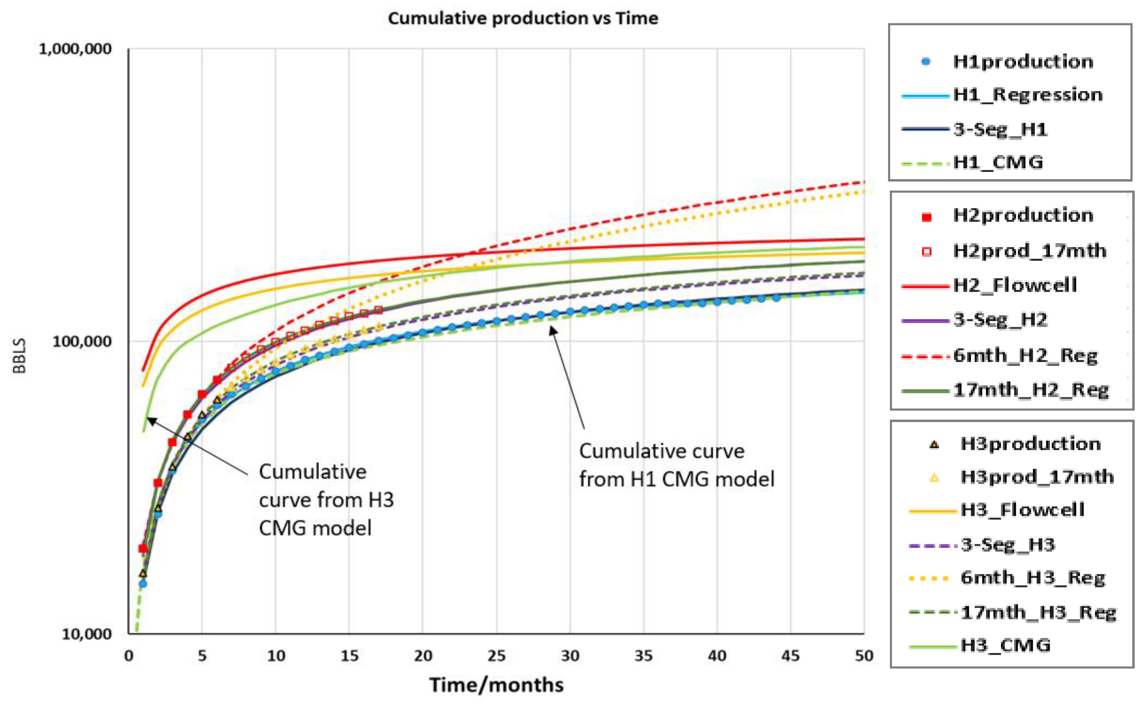
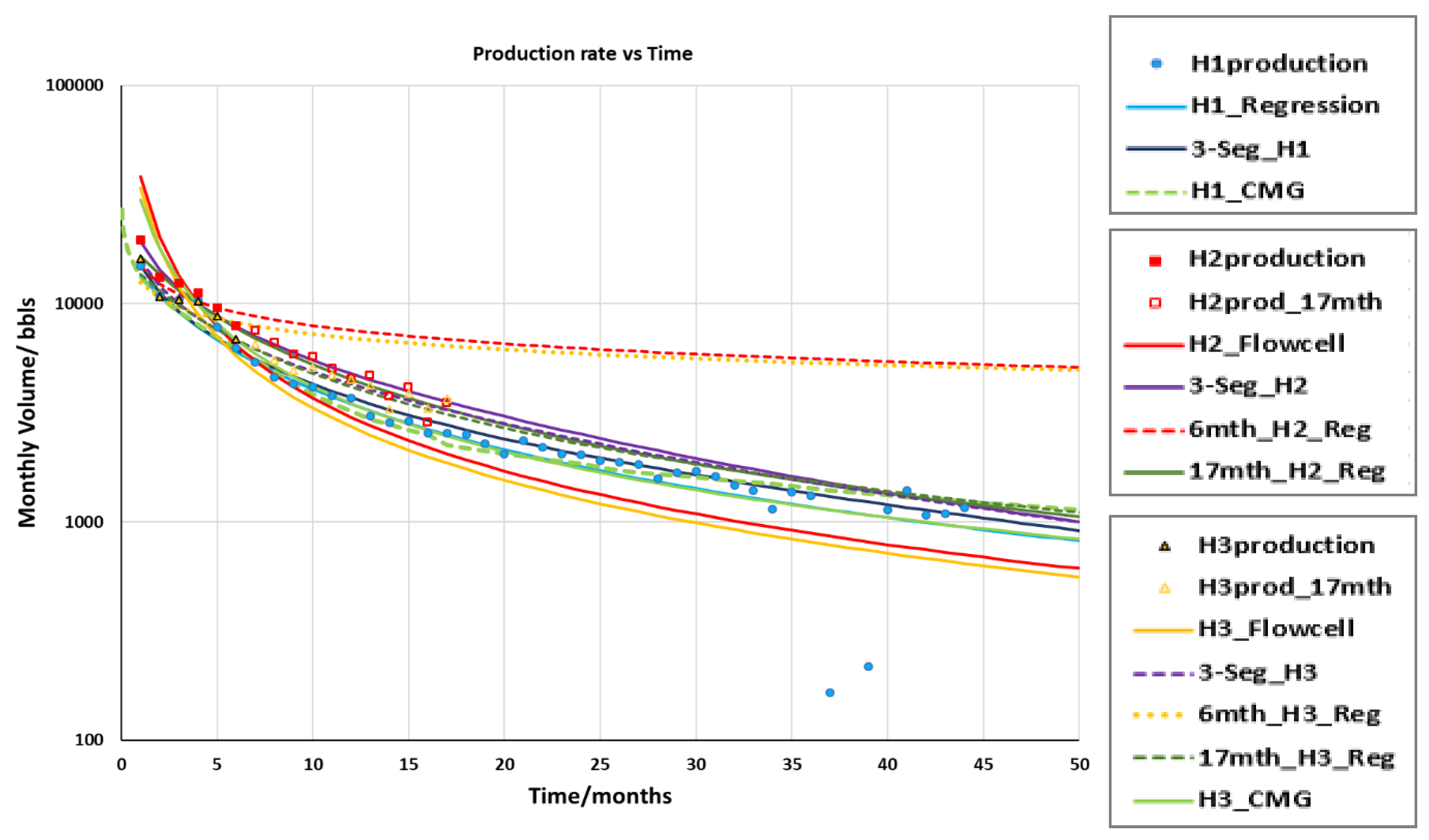
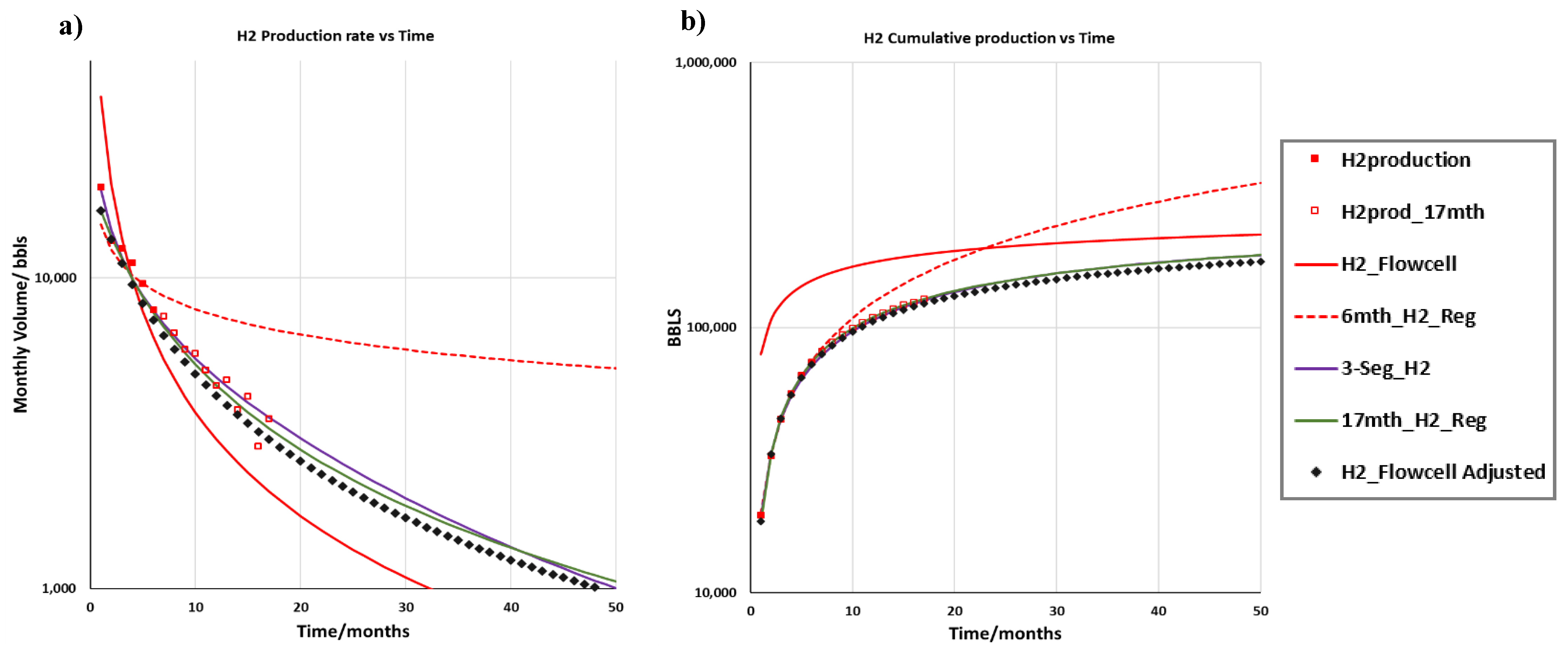
  • The flow cell model does not accurately match the actual production of the H2 and H3 wells in early production time.
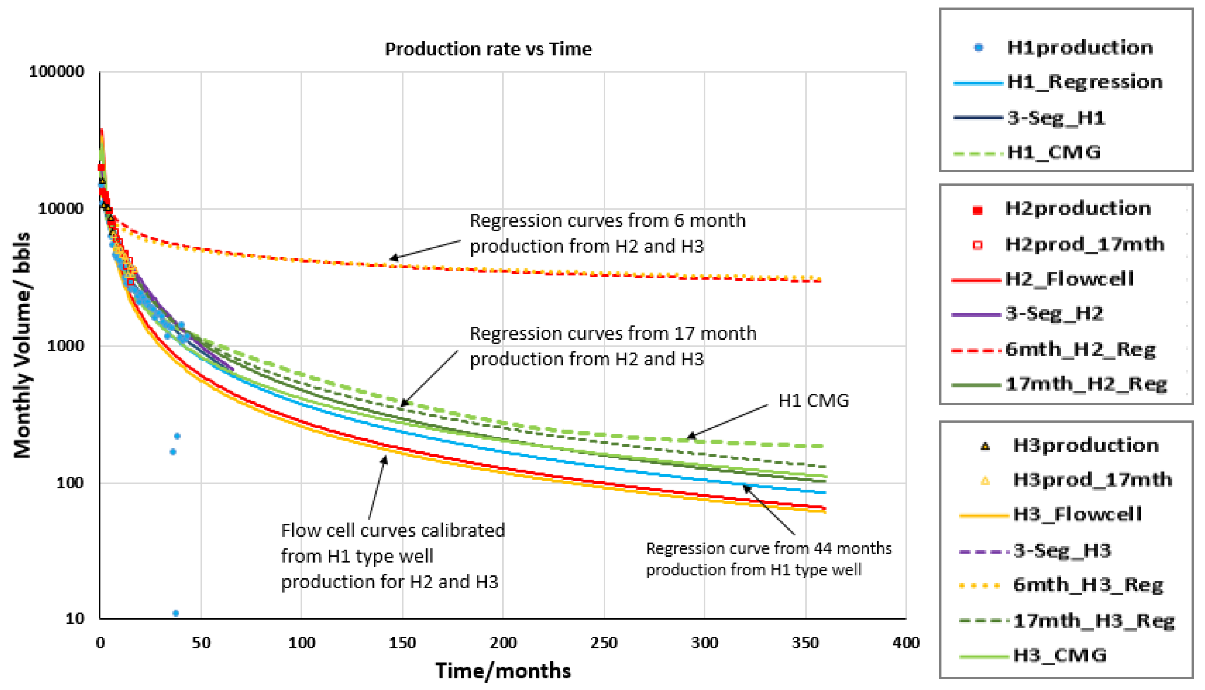
  • The initial production for H2 and H3 from the flow cell model is much greater than the actual production but declines faster and ultimately converges on the H1 EUR forecast.
  • Possible explanation of early time mismatch for flow cell H2 and H3 model is that the intended number of hydraulic fractures was never effectuated due to a number of failed perforation clusters. The ratio of possible failed clusters to total clusters perforated is captured in the newly devised fracture treatment quality factor (TQF).
  • Decline in reservoir pressure from the nearby producing H1 and O wells could be neglected because the pressure transient would not have reached the region hosting H2 and H3 wells at the time of their drilling.
  • H2 and H3 have more hydraulic fractures than H1 but the earlier onset of inter-fracture interference means that the expected uplift in production (compared to H1) from the flow cell model is not realized.

6. Conclusions

The aim of this work was to create a practical tool using analytical expressions to quantify the impact of well interference (due to changes in well spacing and fracture treatment design parameters) on daily production rates and corresponding cumulative volumes from multi-fractured horizontal wells in unconventional reservoirs. The flow-cell model uses a type well for scaling and can forecast the production rate and estimated ultimate recovery (EUR) of newly planned wells, accounting for changes in completion design (frac spacing, height, half-length), total well length, and well spacing. The Excel spreadsheet allows for the quick determination of the impact of hydraulic fracture spacing and inter-well spacing on production rate and on EUR, which is particularly relevant for optimization of field development solutions in unconventional shale and tight carbonate reservoirs.
The flow-cell based 2-segment DCA spreadsheet can be used to quickly determine the optimum fracture and well spacing to obtain the greatest cumulative production within a certain leasehold. A case study presented in this paper, using data from wells from the Eagle Ford Formation, shows this newly developed DCA method matches 30-year EUR estimates within 4% to that calculated by numerical reservoir simulation models. Economic optimization is possible by coupling the flow-cell based 2-segment DCA forecast with a cash flow evaluation spreadsheet to balance the number of wells and production gains possible with the added cost of these wells. An example of such an approach was given by Weijermars and Khanal [6]. By using the Excel spreadsheet in combination with a sound and thorough economic analysis, the greatest value from unconventional assets can be realized.

Author Contributions

Conceptualization, R.W.; Methodology, K.N. and R.W.; Software, K.N. and R.W.; Investigation, K.N.; Writing-Original Draft Preparation, K.N. and R.W.; Writing-Review & Editing, K.N. and R.W.; Supervision, R.W.; Funding Acquisition, R.W. All authors have read and agreed to the published version of the manuscript.

Funding

This project was sponsored by the Crisman-Berg Hughes consortium and startup funds from the Texas A&M Engineering Experiment Station (TEES).

Conflicts of Interest

The authors declare no conflict of interest.

Appendix A. Spreadsheet Interface Guide
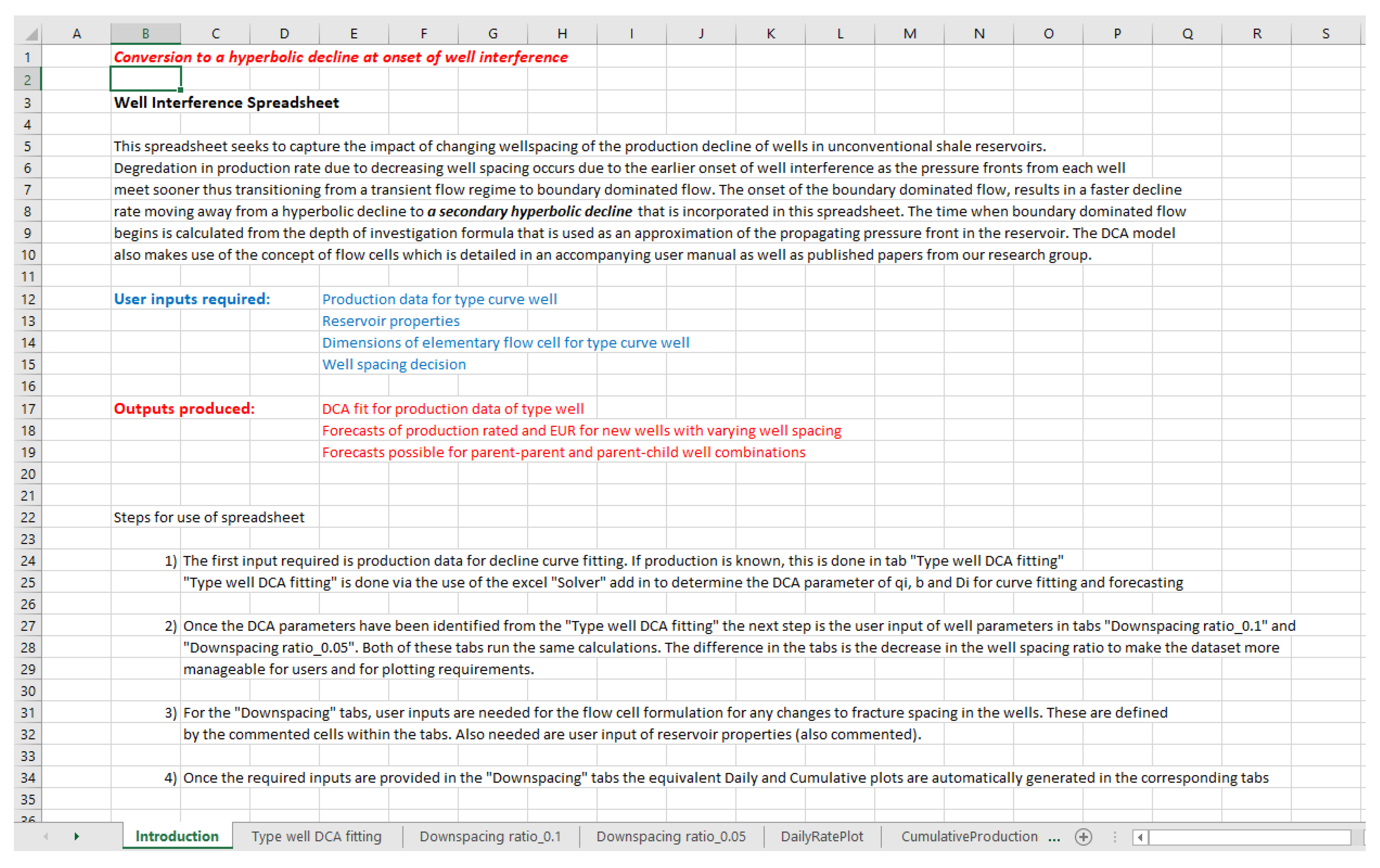
(1)
The first input required is production data for decline curve fitting. If production data are known, this is done in tab “Type well DCA fitting”.
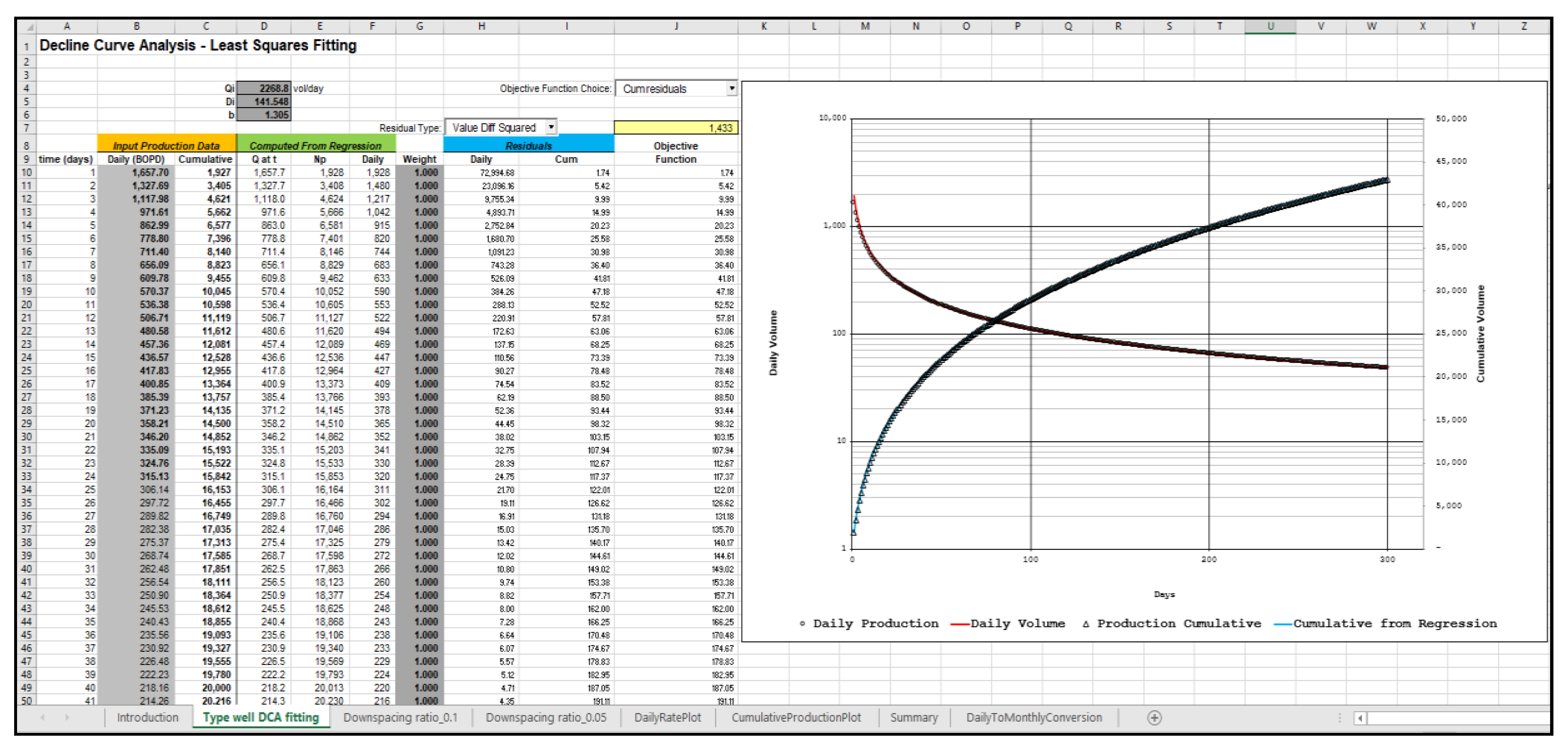
(2)
“Type well DCA fitting” is done via the use of the Excel "Solver" add in to determine the DCA parameter of qi, b, and Di for curve fitting and forecasting.
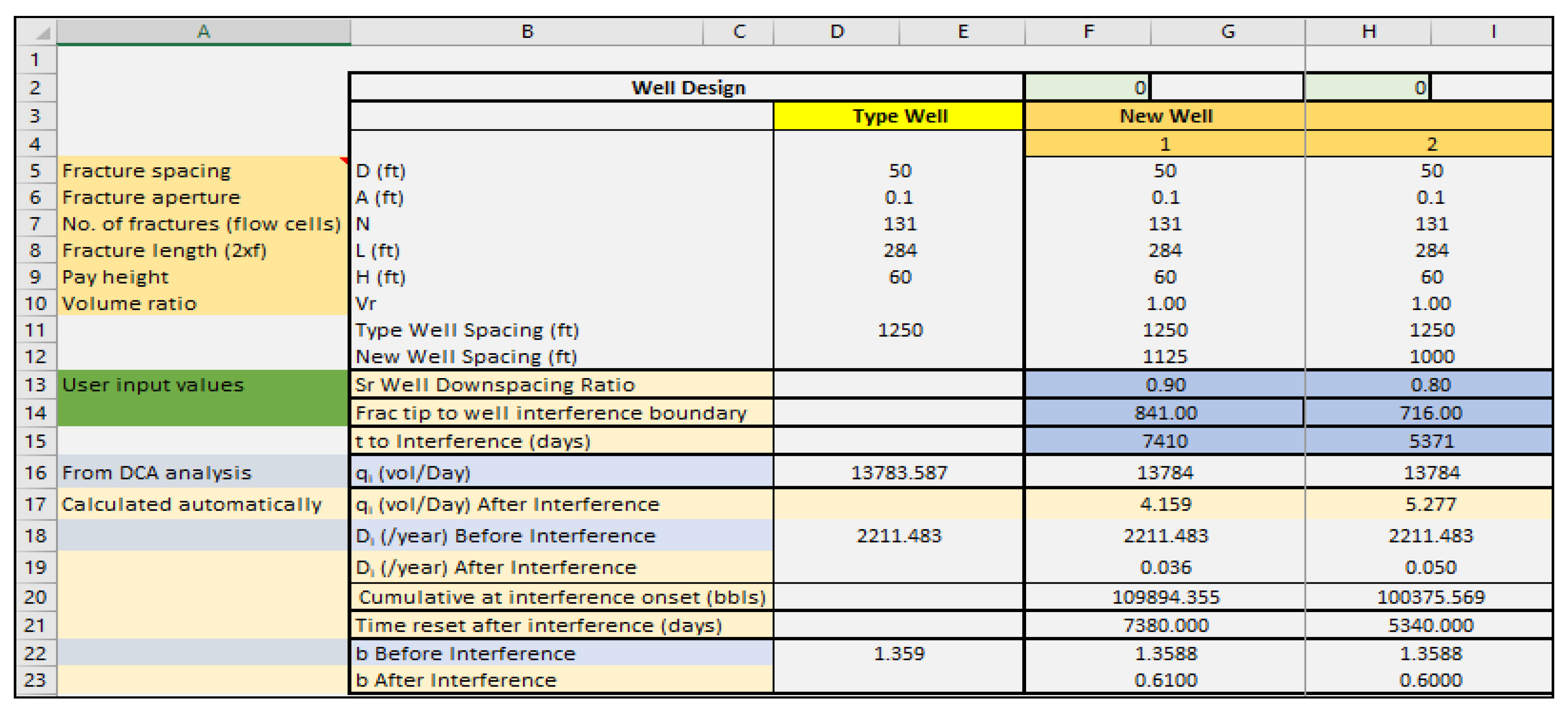
(3)
Once the DCA parameters have been identified from the “Type well DCA fitting” the next step is the user input of well parameters in tabs “Down-spacing ratio_0.1” and “Down-spacing ratio_0.05”. Both of these tabs run the same calculations and refer to fracture down-spacing ratios. Splitting the well spacing ratio over increments with different order of magnitude makes the outputs more manageable for users and for plotting requirements.
(4)
For the “Down-spacing” tabs, user inputs for the flow cell formulation are needed to account for any changes to fracture spacing in the new wells. The required completion dimensions are entered in commented cells in the spreadsheet. User input of reservoir properties (also commented) are also needed.
(5)
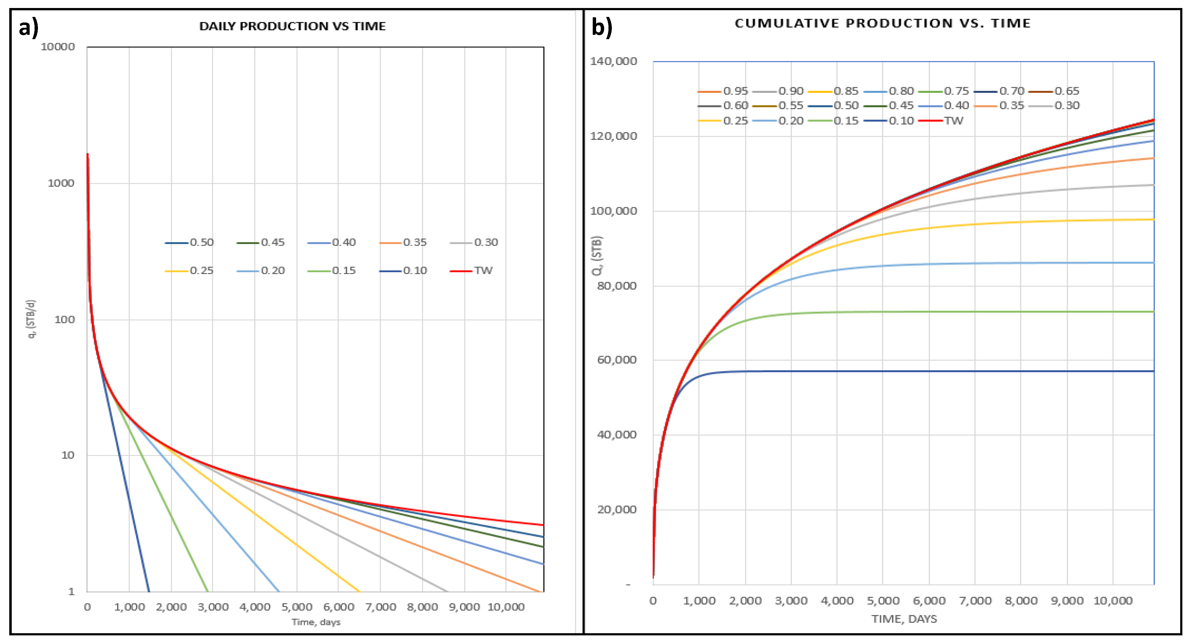
Once the required inputs are provided in the “Down-spacing” tabs, the equivalent Daily and Cumulative plots are automatically generated.
(6)
In addition to completion parameter changes (fracture spacing, height, and half-length), the 2-segment DCA model also accounts for well spacing changes for both simultaneous parent-parent wells as for parent-child wells, with a time delay of their respective drilling and completion.

Appendix A.1. Case Study Example

This section presents a short case example of the use of the Excel spreadsheet created to determine the effects of well interference of production rates and cumulative volumes. We start with the first tab in the spreadsheet named “Introduction” (Figure A1). This tab gives a brief overview of the spreadsheet and how it should be used to generate production forecasts.
Figure A1. Screen capture of the “Introduction” tab.
Energies 13 01525 g0a1
The next step is the DCA curve fitting to production of the type well with spacing sufficient to negate any interference effects. The DCA fitting is used to determine the Qi, b, and Di parameters from the production data in tab “Type well DCA fitting” (Figure A2). If these parameters are already known, this step can be omitted. The match is obtained by varying the parameters to obtain the lowest objective function, which is based on the residual between the actual production data and the forecast. To do this use is made of the Excel Solver add-in. The objective function can be based on either the daily production or cumulative volume and this decision is left up to the user to decide which method gives the best fit.
Figure A2. Screen capture of “Type well DCA fitting” tab to obtain forecast parameter to match type well production data.
Energies 13 01525 g0a2
Once the DCA parameters for the type well are known, we next move on to the “Down-spacing ratio” (shown as “Downspacing” in screen captures) tabs. There are two tabs, the first of which decreases the Down-spacing ratio in increments of 0.1 and the second by increments of 0.5. These ratios are converted into equivalent well spacing distance in feet by knowing the original well spacing of the type curve well. These tabs require user inputs for flow cell dimensions as well as the previously calculated DCA parameters (Figure A3).
Figure A3. Screen capture of the cells requiring user input in the “Down-spacing ratio” tab with additional columns showing down-spacing well values alongside type well values.
Energies 13 01525 g0a3
If the new wells have different fracture, spacing changes can also be made in the subsequent well definitions in this tab. What is also required for the calculation of the onset of well interference (and thus change in flow regime, which affects production rate) are reservoir properties. These user defined reservoir property inputs (Figure A4) are also captured within the “Down-spacing ratio” tab.
Figure A4. Input cells for reservoir properties in the “Down-spacing ratio” tab.
Energies 13 01525 g0a4
With these necessary inputs in the Down-spacing tab, using the depth of investigation formula we can determine the time to the onset of well interference die to different possible well spacing. The forecasted results in the “Down-spacing ratio” tab for all ratios are then carried into the “Daily Rate Plot” and “Cumulative Production Plot” tab for a graphical representation of the impact of various well spacing distances on rates and cumulative volumes (Figure A5).
Figure A5. (a) Daily production rate from different well spacing, (b) cumulative production from different well spacing. ‘TW’ represents type well production with no impact from well interference.
Energies 13 01525 g0a5

Appendix A.2. Methodology Used for Spreadsheet Calculations

The flow-cell based 2-segment DCA approach uses a type well production curve generated from an initial history match to production data, that is then scaled based on the number of flow-cells and the new well spacing. To account for earlier onset of well interference due to decrease in the well spacing, the initial hyperbolic decline segment is switched to a secondary hyperbolic decline segment at different kick-off times. This study has shown that the kick-off time from a detailed KAPPA simulation model can be accurately matched by a simple depth of investigation formula (Figure 13).
The question becomes, at the onset of well interference and thus start of the secondary hyperbolic decline, what is the new ‘b’ parameter to be used and how can it be easily determined. Using the KAPPA model, the secondary hyperbolic decline at the onset of interference is matched in the flow-cell model by varying b-values to get the best fit of the flow-cell production decline to the KAPPA simulation data. From this match, correlations between the ideal b-values needed after well interference onset have been determined (Figure A6).
The first correlation (Figure A6) shows the relation between the best-matched b-values to the kick-off time due to the onset of well interference. As the time of this kick-off is determined by the decrease in well spacing, a second correlation relating the best-matched b-value for the secondary hyperbolic decline with the corresponding down-spacing ratio is easily determined (Figure A7). This correlation can be represented by the equation of the best-fit line presented in Figure A7 and gives a method by which to predict the best b-value for the secondary hyperbolic decline by simply using the well down-spacing ratio.
Figure A6. Correlation of b-value match for secondary hyperbolic decline with corresponding kick-off times due to differing well spacing.
Energies 13 01525 g0a6
Figure A7. Correlation of b-value match for secondary hyperbolic decline with corresponding well spacing ratio.
Energies 13 01525 g0a7

References

  1. Weijermars, R.; Yu, W.; Khanal, A. (Eds.) Improved Reservoir Models and Production Forecasting Techniques for Multi-Stage Fractured Hydrocarbon Wells; MDPI Energies, Book with Collection of 10 Best Papers Special Issue. mdpi.com/books/pdfview/book/1890; MDPI: Basel, Switzerland, 2019; ISBN1 978-3-03921-892-9. ISBN2 978-3-03921-893-6. [Google Scholar]
  2. Weijermars, R.; Johnson, A.; Denman, J.; Salinas, K.; Kennedy, M.; Williams, J. Creditworthiness of North American Oil Companies and Minsky Effects of the (2014–2016) Oil Price Shock. J. Financ. Account. 2018, 6, 162–180. [Google Scholar] [CrossRef]
  3. SPE Taskforce Final Report, 2016. Unconventional Reserves Task Force, The Woodlands, TX, USA, 18–19 August 2015. Available online: https://www.spwla.org/Documents/SPWLA/TEMP/Unconventional%20Taskforce%20Final%20Report.pdf (accessed on 21 March 2020).
  4. Hu, Y.; Weijermars, R.; Lihua, Z.; Yu, W. Benchmarking EUR Estimates for Hydraulically Fractured Wells with and without Fracture Hits Using Various DCA Methods. J. Pet. Sci. Eng. 2017, 162, 617–632. [Google Scholar] [CrossRef]
  5. Tugan, F.M.; Weijermars, R. Improved EUR Prediction for Multi-Fractured Hydrocarbon Wells Based on 3-Segment DCA: Implication for Production Forecasting of Parent and Child Wells. J. Pet. Sci. Eng. 2020, 187, 106692. [Google Scholar] [CrossRef]
  6. Weijermars, R.; Khanal, A. Production Interference of Hydraulically Fractured Hydrocarbon Wells: New Tools for Optimization of Productivity and Economic Performance of Parent and Child Wells. In Proceedings of the SPE Europec featured at 81st EAGE Conference and Exhibition, London, UK, 3–6 June 2019. SPE-195544-MS. [Google Scholar]
  7. Weijermars, R.; Tugan, F.M.; Khanal, A. Production Rates and EUR Forecasts for Interfering Parent-Parent Wells and Parent-Child Wells: Fast Analytical Solutions and Validation with Numerical Reservoir Simulators. J. Pet. Sci. Eng. 2020, 190, 107032. [Google Scholar] [CrossRef]
  8. Ilk, D.; Perego, A.D.; Rushing, J.A.; Blasingame, T.A. Integrating Multiple Production Analysis Techniques to Assess Tight Gas Sand Reserves: Defining a New Paradigm for Industry Best Practices. In Proceedings of the CIPC/SPE Gas Technology Symposium 2008 Joint Conference, Calgary, AB, Canada, 16–19 June 2008. [Google Scholar] [CrossRef]
  9. Ilk, D.; Rushing, J.A.; Perego, A.D.; Blasingame, T.A. Exponential vs. Hyperbolic Decline in Tight Gas Sands—Understanding the Origin and Implication for Reserve Estimates Using Arps’ Decline Curves. In Proceedings of the SPE Annual Technical Conference and Exhibition, Denver, CO, USA, 21–24 September 2008. [Google Scholar] [CrossRef]
  10. Valko, P.P. Assigning Value to Stimulation in the Barnett Shale: A Simultaneous Analysis of 7000 Plus Production Histories and Well Completion Records. In Proceedings of the SPE 119369, SPE Hydraulic Technology Conference, The Woodlands, TX, USA, 19–21 January 2009. [Google Scholar] [CrossRef]
  11. Duong, A.N. Rate-Decline Analysis for Fracture-Dominated Shale Reservoirs. SPE Reserv. Eval. Eng. 2011, 14, 377–387. [Google Scholar] [CrossRef] [Green Version]
  12. Clark, A.J.; Lake, L.W.; Patzek, T.W. Production Forecasting with Logistic Growth Models. In Proceedings of the SPE Annual Technical Conference and Exhibition, Denver, CO, USA, 30 October–2 November 2011. paper SPE 144790. [Google Scholar] [CrossRef] [Green Version]
  13. Patzek, T.W.; Male, F.; Marder, M. Gas Production in the Barnett Shale Obeys a Simple Theory. Proc. Natl. Acad. Sci. USA 2013, 110, 19731–19736. [Google Scholar] [CrossRef] [PubMed] [Green Version]
  14. Zhang, H.; Cocco, M.; Rietz, D.; Cagle, A.; Lee, J. An Empirical Extended Exponential Decline Curve for Shale Reservoirs. In Proceedings of the SPE Annual Technical Conference and Exhibition, Houston, TX, USA, 28–30 September 2015. [Google Scholar] [CrossRef]
  15. Holanda, R.W.D.; Gildin, E.; Valko, P.P. Combining Physics, Statistics, and Heuristics in the Decline-Curve Analysis of Large Data Sets in Unconventional Reservoirs. SPE Reserv. Eval. Eng. 2018, 21, 683–702. [Google Scholar] [CrossRef]
  16. Miao, Y.; Li, X.; Lee, J.; Zhou, Y.; Wu, K.; Sun, Z.; Liu, S. A new rate-decline analysis of shale gas reservoirs: Coupling the self-diffusion and surface diffusion characteristics. J. Pet. Sci. Eng. 2018, 163, 166–176. [Google Scholar] [CrossRef]
  17. Tugan, F.M.; Weijermars, R. Variation in b-sigmoids with flow regime transitions in support of a New 3-Segment DCA Method: Improved Production Forecasting for tight oil and gas wells. J. Pet. Sci. Eng. 2020, in press. [Google Scholar]
  18. Gakhar, K.; Rodionov, Y.; Defeu, C.; Shan, D.; Malpani, R.; Ejofodomi, E.; Fischer, K.; Hardy, B. Engineering an Effective Completion and Stimulation Strategy for In-Fill Wells. In Proceedings of the SPE Hydraulic Fracturing Technology Conference and Exhibition, The Woodlands, TX, USA, 24–26 January 2017. [Google Scholar] [CrossRef]
  19. Bansal, N.; Han, J.; Shin, Y.; Blasingame, T. Reservoir Characterization to Understand Optimal Well Spacing; A Wolfcamp Case Study. In Proceedings of the Unconventional Resources Technology Conference, Houston, TX, USA, 23–25 July 2018. [Google Scholar] [CrossRef]
  20. Khodabakhshnejad, A.; Zeynal, A.R.; Fontenot, A. The Sensitivity of Well Performance to Well Spacing and Configuration—A Marcellus Case Study. In Proceedings of the Unconventional Resources Technology Conference, Denver, CO, USA, 22–24 July 2019. [Google Scholar] [CrossRef]
  21. Lougheed, D.; Behmanesh, H.; Anderson, D. Does Depletion Matter? A Child Well Workflow. In Proceedings of the Unconventional Resources Technology Conference, Denver, CO, USA, 22–24 July 2019. [Google Scholar] [CrossRef]
  22. Izadi, G.; Guises, R.; Barton, C.; Randazzo, S.; Mahrooqi, S.; Shaibani, M.; Dobroskok, A. Advanced Integrated Subsurface 3D Reservoir Model for Multistage Full-Physics Hydraulic Fracturing Simulation. In Proceedings of the International Petroleum Technology Conference, Dhahran, Saudi Arabia, 13–15 January 2020. [Google Scholar] [CrossRef]
  23. Cipolla, C.; Litvak, M.; Prasad, R.S.; McClure, M. Case History of Drainage Mapping and Effective Fracture Length in the Bakken. In Proceedings of the SPE Hydraulic Fracturing Technology Conference and Exhibition, The Woodlands, TX, USA, 4–6 February 2020. [Google Scholar] [CrossRef]
  24. Fowler, G.; McClure, M.; Cipolla, C. A Utica Case Study: The Impact of Permeability Estimates on History Matching, Fracture Length, and Well Spacing. In Proceedings of the SPE Annual Technical Conference and Exhibition, Calgary, AB, Canada, 30 September–2 October 2019. [Google Scholar] [CrossRef]
  25. Yu, W.; Wu, K.; Zuo, L.; Tan, X.; Weijermars, R. Physical Models for Inter-Well Interference in Shale Reservoirs: Relative Impacts of Fracture Hits and Matrix Permeability. In Proceedings of the SPE Unconventional Resources Technology Conference, San Antonio, TX, USA, 1–3 August 2016. SPE-URTeC 2457663. [Google Scholar] [CrossRef] [Green Version]
  26. Yu, W.; Xu, Y.; Weijermars, R.; Wu, K.; Sepehrnoori, K. Impact of Well Interference on Shale Oil Production Performance: A Numerical Model for Analyzing Pressure Response of Fracture Hits with Complex Geometries. In Proceedings of the SPE, Hydraulic Fracturing Conference, Woodlands, TX, USA, 24–26 January 2017. SPE 184825. [Google Scholar]
  27. Yu, W.; Xu, Y.; Weijermars, R.; Wu, K.; Sepehrnoori, K. A numerical model for simulating pressure response of well interference and well performance in tight oil reservoirs with complex fracture geometries using the fast embedded discrete fracture model method. SPE Reserv. Eval. Eng. 2018, 21, 489–502. [Google Scholar] [CrossRef]
  28. Garza, M.; Baumbach, J.; Prosser, J.; Pettigrew, S.; Elvig, K. An Eagle Ford Case Study: Improving an Infill Well Completion Through Optimized Refracturing Treatment of the Offset Parent Wells. In Proceedings of the SPE Hydraulic Fracturing Technology Conference and Exhibition, The Woodlands, TX, USA, 5–7 February 2019. [Google Scholar] [CrossRef]
  29. McClure, M.; Picone, M.; Fowler, G.; Ratcliff, D.; Kang, C.; Medam, S.; Frantz, J. Nuances and Frequently Asked Questions in Field-Scale Hydraulic Fracture Modeling. In Proceedings of the SPE Hydraulic Fracturing Technology Conference and Exhibition, The Woodlands, TX, USA, 4–6 February 2020. [Google Scholar] [CrossRef]
  30. Yang, X.; Yu, W.; Weijermars, R.; Wu, K. Fracture hits via diagnostic charts to assess production interference level. SPE J. 2020, in press. [Google Scholar] [CrossRef]
  31. Parsegov, S.G.; Nandlal, K.; Schechter, D.S.; Weijermars, R. Physics-Driven Optimization of Drained Rock Volume for Multistage Fracturing: Field Example from the Wolfcamp Formation, Midland Basin. SPE-URTeC: 2879159. In Proceedings of the Unconventional Resources Technology Conference, Houston, TX, USA, 23–25 July 2018. [Google Scholar] [CrossRef] [Green Version]
  32. Coveney, P.V.; Dougherty, E.R.; Highfield, R.R. Big data need big theory. Philos. Trans. R. Soc. A 2016, 374, 20160153. [Google Scholar] [CrossRef] [PubMed]
  33. Weijermars, R.; Nascentes Alves, I. High-Resolution Visualization of Flow Velocities Near Frac-Tips and Flow Interference of Multi-Fracked Eagle Ford Wells, Brazos County, Texas. J. Pet. Sci. Eng. 2018, 165, 946–961. [Google Scholar] [CrossRef]
  34. Arps, J.J. Analysis of Decline Curves. Trans. AIME 1945, 160, 228–247. Available online: https://www.onepetro.org/journal-paper/SPE-945228-G. [CrossRef]
  35. Khanal, A.; Weijermars, R. Pressure depletion and drained rock volume near hydraulically fractured parent and child wells. J. Pet. Sci. Eng. 2019, 172, 607–626. [Google Scholar] [CrossRef]
  36. Weijermars, R.; Nandlal, K.; Khanal, A.; Tugan, M.F. Comparison of Pressure Front with Tracer Front Advance and Principal Flow Regimes in Hydraulically Fractured Wells in Unconventional Reservoirs. J. Pet. Sci. Eng. 2019. [Google Scholar] [CrossRef]
  37. Maley, S. The Use of Conventional Decline Curve Analysis in Tight Gas Well Applications. In Proceedings of the SPE/DOE (Society of Petroleum Engineers and U.S. Department of Energy), Low Permeability Gas Reservoirs, Denver, CO, USA, 19–22 May 1985. [Google Scholar] [CrossRef]
Figure 1. (a) Principle sketch of flow cells in single well. Blue lines are streamlines in flow cell between two sub-parallel hydraulic fractures. (b) Three flow cells in a partial section of a single horizontal well. Dashed lines are flow separation surface. Yellow dots represent stagnation points. D is fracture spacing, H pay height, and L hydraulic fracture length. After [7].
Energies 13 01525 g001
Figure 2. (a) Principle sketch of flow separation surfaces between closely spaced, horizontal wells. Vertical fractures are transverse to the wellbore. Flow separation surfaces will also occur between individual fracture planes. Liquid migration from the matrix will approach bi-linear flow near the hydraulic factures. Flow in the fracture planes will be radial toward the perforation zones of the wellbore. (b) Flow separation surfaces can be distinguished into Interwell Drainage Boundaries (IDB), Transverse Flow Separation Boundaries (TFSB), and Longitudinal Flow Separation Boundaries (LFSB). After [7].
Energies 13 01525 g002
Figure 3. Workflow for optimizing fracture spacing and well spacing given particular acreage dimensions. Process can be repeated for selected type wells to determine the optimized net present value (NPV) for the entire field. After [6].
Energies 13 01525 g003
Figure 4. Long-term production forecasts. (a) Monthly production rates for H1 well for 44 months data (H1production) with corresponding forecasts from a simple regression (H1_Regression), 3-segment decline curve (3-Seg_H1) and CMG reservoir simulation (H1_CMG). (b) Cumulative production for H1 well for 44 months data with corresponding cumulative forecasts from a simple regression, 3-segment decline curve and CMG reservoir simulation (same legends as in (a)).
Energies 13 01525 g004
Figure 5. Short-term production forecasts. (a) Enhanced view of monthly production rates for H1 well for 44 months data (H1production) with corresponding forecasts from a simple regression (H1_Regression), 3-segment decline curve (3-Seg_H1) and CMG reservoir simulation (H1_CMG). (b) Enhanced view of cumulative production for H1 well for 44 months data with corresponding cumulative forecasts from a simple regression, 3-segment decline curve and CMG reservoir simulation (same legends as in (a)).
Energies 13 01525 g005
Figure 6. Comparison of wells H1, H2, and H3 cumulative production data with long-term production forecasts from 1) Arps regressions (using both 6 months and 17 months production data), 2) Analytical flow-cell model, 3) 3-segment Decline Curve and 4) CMG model (for H1 and H3 wells only). Legend explained as follows (each box represents curves modeled for a single well): H1production—44 month H1 well production, H1_Regression—Arps regression on 44 months historical data, 3-Seg_H1—3 segment decline curve based on 44 months production data, H1_CMG —production forecast for H1 from CMG reservoir simulation, H2production—H2 6 month production, H2prod_17mth—H2 production data updated to 17 months, H2_Flowcell—production forecast from flow cell model based on H1 44 month regression fit, 3-Seg_H2—3 segment decline based on 17 month H2 production, 6mth_H2_Reg—Arps regression on 6 month H2 production data, 17mth_H2_Reg—Arps regression on 17 month H2 production data, H3production—H3 6 month production, H3prod_17mth—H3 production data updated to 17 months, H3_Flowcell—production forecast from flow cell model based on H1 44 month regression fit, 3-Seg_H3—3 segment decline based on 17 month H3 production, 6mth_H3_Reg—Arps regression on 6 month H3 production data, 17mth_H3_Reg—Arps regression on 17 month H3 production data, H3_CMG—production forecast for H3 from CMG reservoir simulation.
Energies 13 01525 g006
Figure 7. Enhanced view of the short-term comparisons of wells H1, H2, and H3 cumulative production data with short-term production forecasts from 1) Arps regressions (using both 6 months and 17 months production data), 2) Analytical flow-cell model, 3) 3-segment Decline Curve and 4) CMG model (for H1 and H3 wells only). Legend description follows from Figure 6.
Energies 13 01525 g007
Figure 8. Long-term production forecasts for monthly production rates of Wells H1, H2, and H3, from (1) Arps regressions (using both 6 months and 17 months production data), (2) analytical flow-cell model, (3) 3-segment Decline Curve, and (4) CMG model (for H1 and H3 wells only).
Energies 13 01525 g008
Figure 9. Enhanced view of short-term production rate forecasts for Wells H1, H2, and H3 monthly production data with forecasts from (1) Arps regressions (using both 6 months and 17 months production data), (2) analytical flow-cell model, (3) 3-segment Decline Curve, and (4) CMG model (for Wells H1 and H3 only).
Energies 13 01525 g009
Figure 10. (a) Monthly production for H2 well with corresponding forecasts from different methods and the introduction of an adjusted flow-cell forecast making use of the fracture treatment quality factor (TQF) (H2_Flowcell adjusted). (b) Cumulative production for H2 well with corresponding forecasts from different methods and the introduction of an adjusted flow-cell forecast making use of the well TQF (H2_flow-cell adjusted).
Energies 13 01525 g010
Figure 11. (a) Three-dimensional (3D) numerical model and the gridding built to generate rate data for well to type well (W/TW) cases. The model presents the pressure distribution at the final time step (30 years) of the constant pressure production simulation for W/TW = 1.0 case. (b) Map view of the numerical reservoir model used for the W/TW = 1.0 case. After [7].
Energies 13 01525 g011
Figure 12. Numerical (KAPPA) model forecasts. (a) Cumulative production, and (b) log rate versus time plot, for W/TW = 1.0 to W/TW = 0.3 cases. After [7].
Energies 13 01525 g012
Figure 13. Kick-off times due to onset of well interference for different well spacing using (1) depth of investigation (DOI) equation from wellbore, (2) DOI formula from hydraulic fracture tip, and (3) KAPPA simulation model.
Energies 13 01525 g013
Figure 14. Flow-cell based forecasts. (a) Cumulative production, and (b) log rate versus time plot, for W/TW = 1.0 to W/TW = 0.3 cases.
Energies 13 01525 g014aEnergies 13 01525 g014b
Figure 15. Log-log rate versus time plots for various well spacing with W/TW ranging between 1.0 to 0.3. After [7].
Energies 13 01525 g015
Figure 16. Analysis of b-sigmoids in log-log rate versus time plots. (a) W/TW = 1.0, (b) W/TW = 0.7. After [7]. For further details on b-sigmoids, see [17].
Energies 13 01525 g016
Table 1. Effective lateral length, fracture spacing, fracture number, and total proppant injected for the Eagle Ford Wells H1, H2, and H3.
Well NameLateral LengthNumber of StagesStage SpacingTotal Perf Clusters Fracture/Cluster SpacingTotal Proppant
-ft-ft-ftlbs
Well H16550223001315010,664,970
Well H279055145–18043318N/A
Well H373595056–17741318N/A
Table 2. Comparison of 30-year estimated ultimate recovery (EUR) estimates for Wells H1, H2, and H3 from various methods.
Well NameArps Hyperbolic DCA
(44 mth H1 & 6mth H2 & H3) Regression (Mstb)
Arps Hyperbolic DCA (17mth) Regression (Mstb)Flow Cell Model Based on H1 Type Well (Mstb)3-segment DCA (Limited) Historical Production Data (Mstb)3-Segment DCA
(+4 Months Data) (Mstb)
3-Segment DCA
(+Initial Rate) (Mstb)
CMG Model (Mstb)
H1218----209266
H21,476277278248282228-
H31,470274250228-204291
Table 3. Corresponding kick-off times for onset of well interference for different well spacings using (1) DOI formula with pressure transient starting from horizontal wellbore, and (2) DOI formula with pressure transient starting from hydraulic fracture tips.
Well SpacingW/TW RatioKick-Off Time
(DOI Formula from Wellbore)
Kick-Off Time
(DOI Formula from Fracture Tips)
ft-MonthsMonths
11250.9435243
10000.8344176
8750.7263120
7500.619375
6250.513440
5000.48616
3750.3483
Table 4. History matched b values for given KAPPA model kick-off times with decreasing well spacing.
Well SpacingW/TW RatioKick-Off Time
(KAPPA Model)
b Value Match
ft-Months-
11250.92590.61
10000.81660.60
8750.71150.59
7500.6830.57
6250.5380.52
5000.4180.37
3750.360.26
Table 5. EUR Comparison between KAPPA and Hyperbolic Flow cell model (DOI frac-tip kick-off times).
Well Spacing (W/TW)KAPPA Model EUR
(bbls)
Flow-Cell Hyperbolic Model EUR
(bbls)
Percentage Difference from KAPPA Model
1122,699122,190−0.41%
0.9123,103122,074−0.84%
0.8121,148121,4630.26%
0.7118,063119,6711.36%
0.6112,496115,2882.48%
0.5101,372105,3633.94%
0.483,93882,193−2.08%
0.360,25558,402−3.08%

