Mapping of the Temperature–Entropy Diagrams of van der Waals Fluids

Abstract

The shape of the temperature vs. specific entropy diagram of a working fluid is very important to understanding the behavior of fluid during the expansion phase of the organic Rankine cycle or similar processes. Traditional wet-dry-isentropic classifications of these materials are not sufficient; several materials remain unclassified or misclassified, while materials listed in the same class might show crucial differences. A novel classification, based on the characteristic points of the T–s diagrams was introduced recently, listing eight different classes. In this paper, we present a map of these classes for a model material, namely, the van der Waals fluid in reduced temperature (i.e., reduced molecular degree of freedom) space; the latter quantity is related to the molar isochoric specific heat. Although van der Waals fluid cannot be used to predict material properties quantitatively, the model gives a very good and proper qualitative description. Using this map, some peculiarities related to T–s diagrams of working fluids can be understood.

1. Introduction

Organic Rankine cycles (ORCs), where the traditional water/steam pair is replaced by an organic liquid/vapor pair, are very important in the utilization of low-temperature heat sources. In this way, even at relatively low temperatures, one can create organic vapor with sufficiently high pressure to drive turbines or expanders [1].

The selection of a proper working fluid is an important, multi-dimensional optimization problem [2]. Thermodynamical (e.g., efficiency), chemical (e.g., corrosion), biological (e.g., toxicity), environmental (e.g., global warming potential (GWP) and ozone depletion potential (ODP)), and other issues have to be considered with different weight [3,4]. For thermodynamic considerations, working fluids can be divided into several classes, depending on their behavior during the adiabatic expansion step of the ORC. Traditional classification uses three categories, namely wet, dry, and isentropic [2]. For wet fluids, starting the expansion from a saturated vapor state, the final state of an ideal (reversible adiabatic, i.e., isentropic) expansion is always a mixed, wet fluid state (droplets dispersed in the vapor). The presence of droplets should be avoided because they can damage the expanders; this can be done by the application of a superheater or droplet separator. For dry fluids, a similar expansion—except for those starting in the vicinity of the critical point—always ends in the dry, superheated vapor region. The presence of the superheated vapor requires greater cooling capacity from the condenser or the use of a recuperative or regenerative heat exchanger [5]. For isentropic fluids, the expansion would run along (or slightly above) the saturated vapor line, avoiding the previously mentioned problems. Unfortunately, isentropic fluids with an extended constant-entropy part on the saturated vapor branch do not exist; this part is always tilted or reverse S-shaped [6,7,8]. Concerning T–s (temperature–specific entropy) diagrams, the slope of the saturated vapor curve (the part of T–s diagram located on the high-entropy side of the critical point) is always negative for wet classes, always positive (except a tiny negative region close to the critical point) for dry ones, and theoretically would be infinite (except a tiny negative region close to the critical point) for isentropic ones [9,10,11].

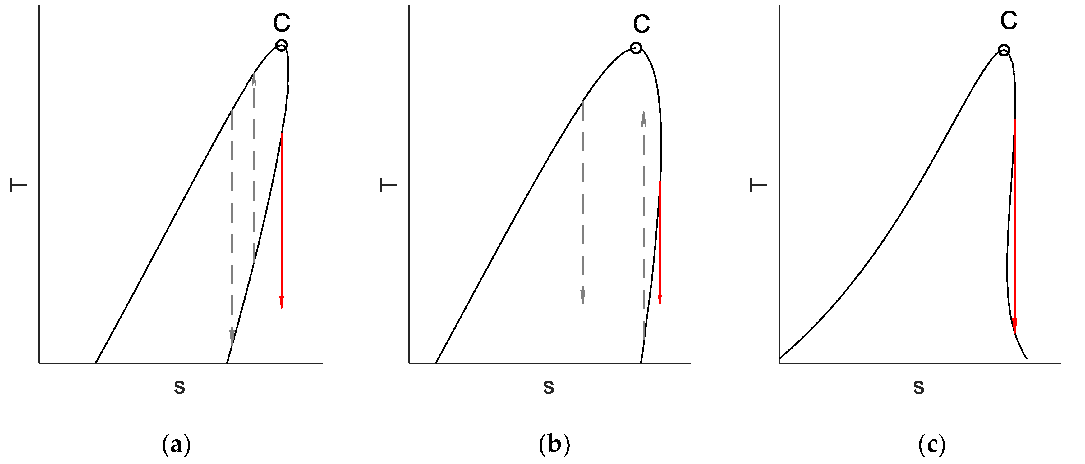
There are several disadvantages to this traditional classification: two of them are shown in Figure 1. In Figure 1a,b, one can see the two schematic T–s (temperature–specific entropy) diagrams of two hypothetical dry fluids. One can clearly see that although according to the previously mentioned criterium (isentropic expansion from a saturated vapor state terminated in dry vapor region, shown by solid red arrows) both fluids are dry, still, they have considerable differences. The liquid and vapor parts of the saturation curve are separated by the critical point (C), having the liquid part on the low-entropy, and the vapor part on the high-entropy side. One of the important difference is that in the case of Figure 1a, there is a theoretical possibility to fully transform the fluid from liquid to vapor and vice versa by pure ideal compression or expansion; In contrast, in the case of Figure 1b, this transformation will be only partial (see dashed arrows). In the first case, the diagram is strongly tilted and therefore for low-temperature saturated vapor states, the entropies are lower than for high-temperature liquid phases (giving the possibility to the afore-mentioned isentropic vapor-to-liquid or liquid-to-vapor transitions), while in the second case, on the entropy-scale, vapor states are always above the liquid ones, disabling the system to fully vaporize or liquefy in an adiabatic step. This example shows that the dry class should be divided into at least two subclasses, depending on the relative position (on the entropy scale) of the critical point and the end-point of the saturated vapor branch.

The other problem is that for real working fluids, one can easily find a T–s diagram with a special shape, not accurately covered by the dry-wet-isentropic classes. This type is shown in Figure 1c. Traditionally, some of the fluids showing this shape were considered as dry (regarding only the upper, high-temperature part) or isentropic (only in cases where the inverse S-shape of the saturated vapor curve was so flat that it was considered as an almost straight, vertical line) while a lot of them were wrongly classified or not classified at all [12]. Practically, fluids showing this behavior can be forced into the isentropic class because it is possible to have an ideal adiabatic “saturated vapor to saturated vapor” expansion (see full arrow) [6]. However, while for theoretical isentropic working fluids (where part of the saturated vapor curve would be a straight, vertical line) it is possible to expand from any temperature to any other in a reversible adiabatic manner (at least within the temperature range, where “isentropicity” would be true), for these reverse S-shaped ones, it is possible to do so only between certain temperature pairs (connecting two points with a vertical line, like on Figure 1c). For a given fluid, these pairs—considered as starting/end-points of ideal expansion steps—can be represented by a curve on an upper vs. lower temperature diagram. These diagrams can be used to select working fluid for a given heat sink/heat source pair [6]. These fluids, due to the existence of isentropic “saturated vapor to saturated vapor” expansion steps (red arrow, Figure 1c), can be referred as “real isentropic” working fluids (distinguishing them from the idealized isentropic ones).

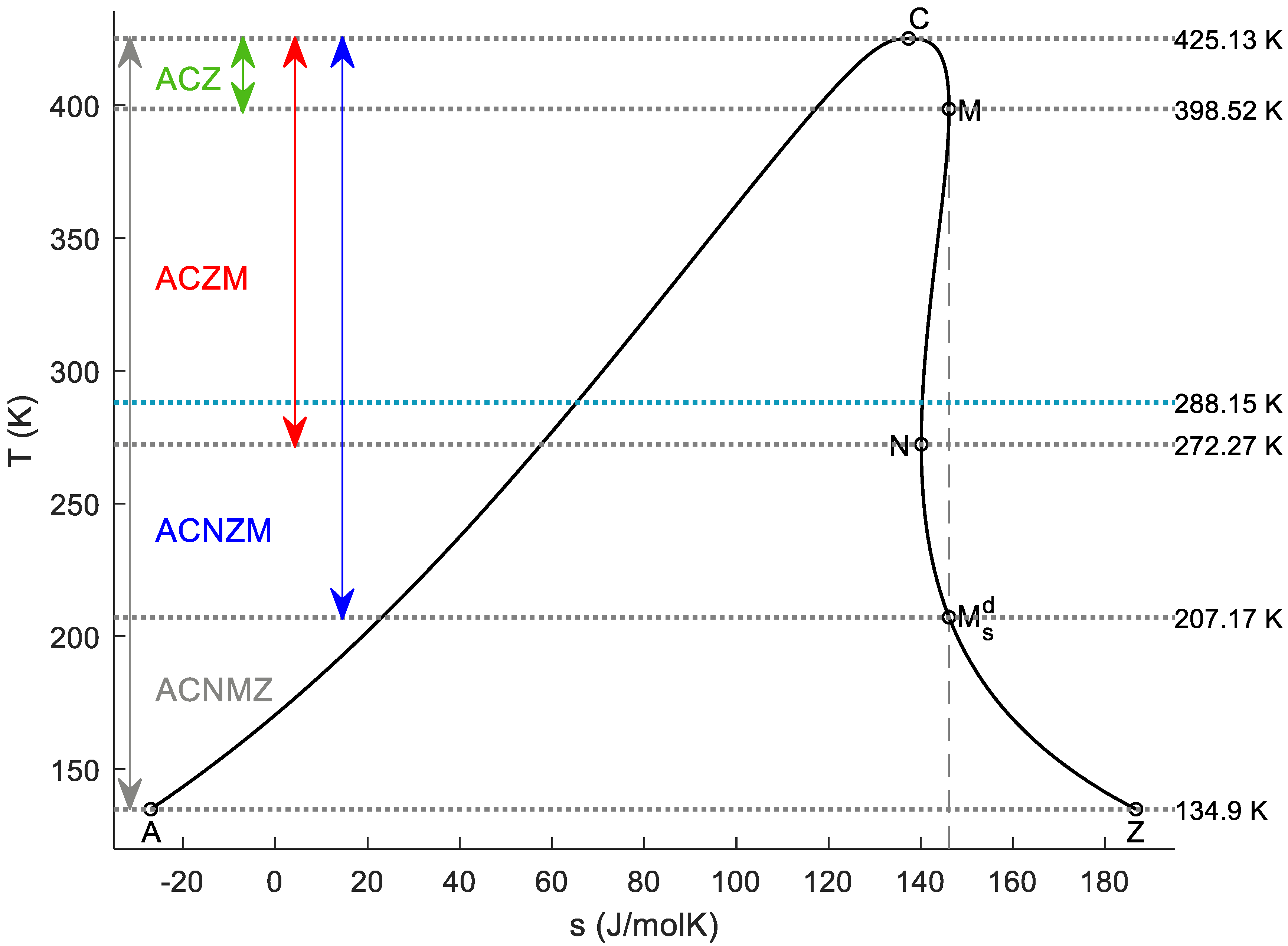
To solve for these shortcomings, a novel classification was introduced [12] based on the entropy sequence of characteristic points on the T–s diagrams. These points (shown in Figure 2) were the two end-points of the curve (marked as A for the low-entropy and Z as the high-entropy side), the critical point (C), and two local extrema on the saturated vapor part, a maximum (M) and a minimum (N). A, C, and Z points exist for all materials, while M and N exist only for the dry or the reverse S-shaped ones. Since that A, C, and Z points are present for all materials, they are called primary characteristic points, while M and N (being present only for the non-wet working fluids) are the secondary characteristic points.

From these five characteristic points, one can theoretically construct 3! + 4! + 5! = 6 + 24 + 120 sequences containing only the primary points (A, C, and Z) or the primaries plus M (A, C, Z, and M) or finally all the five points (A, C, Z, M, and N); it is an enormous number to replace the previously used three classes. Fortunately, due to some constraints (for example, the entropy of point C is always bigger than that for point A, or the entropy of point M is always above the entropy values for points C and N) one can define only eight possible sequences, giving one subclass for wet (ACZ), two subclasses for dry (ACZM and AZCM; the first one is demonstrated in Figure 1b, the second one is in Figure 1a), and five subclasses for the “real isentropic” sequence (ANCMZ, ACNMZ, ANZCM, ANCZM, and ACNZM) [12]. These subclasses are shown in Appendix A, while the classification of some real. pure working fluids (only for the ones having accurate T–s data in the NIST Chemistry Webbook [13]) can be found in the Supplementary Data Section of reference [12].

Taking the two end-points (A and Z) as the absolute end-points of the T–s curves, i.e., locating them to the triple point, the obtained class will be an absolute material property, just like critical temperature, molar mass, etc. On the other hand, these classifications sometimes are not very user-friendly, because the temperature of the triple point sometimes is much below the temperature range applicable in usual ORC processes. Therefore, we introduced a few more characteristic points, called ternary characteristic points [14]. They are created by projecting the primary and secondary points to the T and s axes; here, we are using only the latter ones. The projection line extended along the whole temperature scale can cross the original T–s diagram, defining the ternary points by these intersections. Due to the nature of the projection, the entropy or the temperature of these points coincide with the entropy or temperature of the corresponding primary or secondary characteristic points. For example, by projecting point C to the entropy axis, it might cross the original diagram once or twice, depending on the class of the fluid. These ternary points are marked as $C_s^d$ and $C_s^{dd}$; s index marks the axis where the points are projected, d marks the position of the new ternary point compared to the original point; therefore these points (being d for down) are on temperatures below the temperature of point C. Finally, the number of the upper indices are marking the intersection nearer (one index) or farther (double index) from the original characteristic point. The importance of these points and the temperature-dependent part of this novel classification method is demonstrated through the case of butane (Figure 2); T–s data taken from the NIST Webbook [13].

Butane is a type ACNMZ working fluid; the fluid range extends from the triple-point temperature, 134.90 K (−138.25 °C) to the critical temperature 425.13 K (151.98 °C). One can easily realize that in ORCs it is quite unlikely that butane would expand down to −138 °C, or even in the vicinity, except for some cryogenic applications [15]. Therefore, it is important to know how the classification can change by fixing the lower end to an environment-given minimal temperature (like 288.15 K = 15 °C), instead of fixing it to the material-given triple-point temperature. In this way, one might realize, that while a working fluid (butane, in this case) might be an ACNMZ-type fluid, in a confined temperature range, it can emulate other types, even an ACZ one. These transitions can be seen in Figure 2. For this fluid class (ACNMZ), the entropy of point N is above the entropy of all saturated liquid states, therefore, projecting point C to the entropy axis would not yield any intersection with the saturated vapor curve. The projection line for N would yield one intersection ($N_s^u$) close to point C, but as will be seen later, this point has no relevance here, therefore it is not shown. The projection line of M (dashed) crosses the saturated vapor line in a point, which is referred to here as $M_s^d$. There are also some dotted lines, marking the temperatures of the primary and secondary points, as well as for this new ternary point. One further temperature is also marked (288.15 K = 15 °C) as the ambient temperature.

As was already mentioned, considering the full fluid range between the triple-point temperature (134.90 K) and critical temperature (425.13 K), butane is a type ACNMZ working fluid; this is shown in Figure 2 with grey characters and the corresponding temperature range is marked with a grey arrow. When, for some practical reason, we are interested only in higher temperature ranges, the situation changes. Butane remains ACNMZ type only up to the temperature of point $M_s^d$, 207.17 K. This means that when we are interested in expansion properties for butane only above this temperature, the butane behaves like an ACNZM-type fluid (instead of the original ACNMZ class), considering the temperature range between points $M_s^d$ and C; this range is shown by a double-headed blue-colored arrow. This happens because the entropy of the new end-point of the saturated vapor curve is now lower than the entropy of point M, therefore, Z exchanges places with M in the sequence (MZ ending turns to ZM, while the first three letters remain intact). In some cases [12], these temperature-dependent end-points are marked with stars (Z*; and because A is also connected to the same temperature, A*); therefore the new class would be A*CNZ*M to show that it is a temperature-dependent class: For the sake of simplicity, we are omitting the stars for now. Increasing the temperature of the new end-point further, reaching point N (at 272.27 K) would cause the butane to behave like a dry, ACZM-type fluid because above that temperature, point N (local entropy minimum) falls below the new end-point (and letter N disappears from the sequence). Increasing the temperature even further, the next class-change happens by reaching point M (398.52 K). Hence, when the operation temperature is between point N to point C (272.27 K to 425.13 K) butane behaves as an ACZM-type fluid (temperature range marked by a red arrow), from point M to point C it behaves like a wet, ACZ-type one (range is shown by a green arrow), although these temperatures (above point M) are hardly used in ORC applications [16]. An extra temperature (288.15 K = 15 °C) marks a plausible ambient temperature, which can be taken as the lower cycle temperature, for example, for an air-cooled geothermal ORC unit. In that case, butane will have a dry, ACZM-type behavior.

Here, one can see a change of sequences: ACNMZ→ACNZM→ACZM→ACZ. For other real materials, these sequences can be different; for example, for water and carbon dioxide, which are ACZ types, the classification remains unchanged by increasing the lower end temperature, while for dodecafluoropentane, the sequence is AZCM→ACZM→ACZ (T–s data for substances are taken from the NIST Webbook [13]). Using data for model fluids (for example, simple van der Waals fluid [5] or Redlich–Kwong fluid [17]) or simply using geometrically correct schematic representations [12], one can make the temperature-dependent sequence change for all the eight types. The figures explaining the changes are in the Appendix A, together with the list of temperature-dependent sequences. 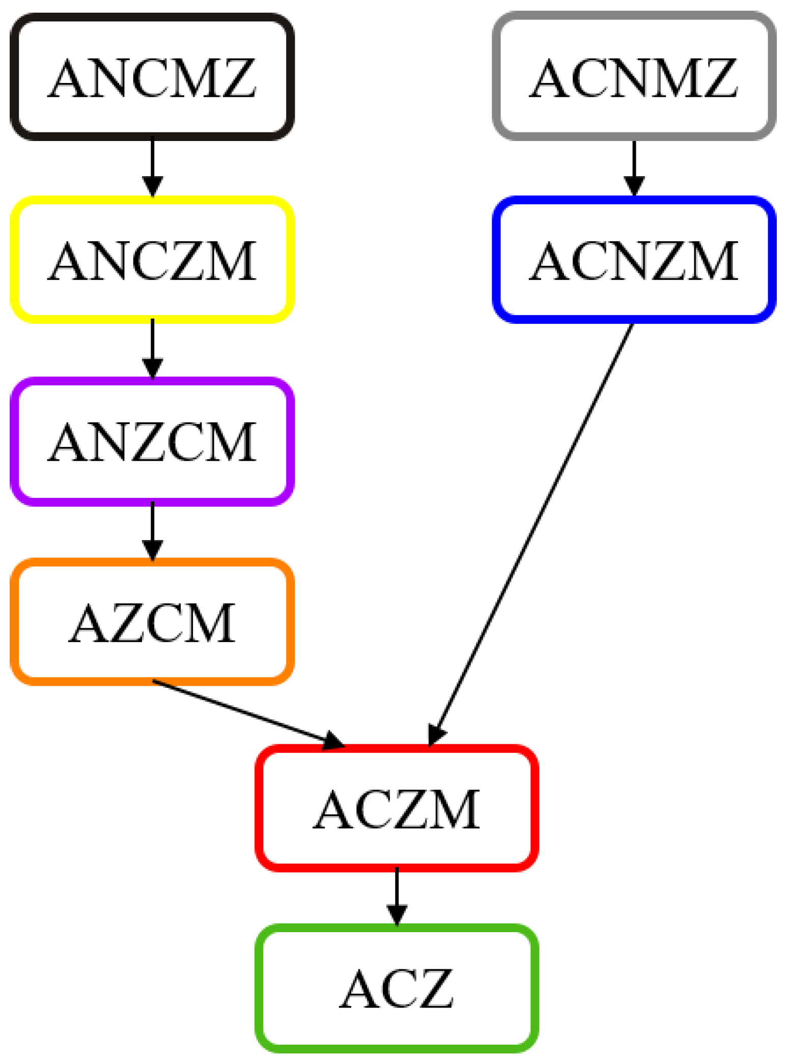For better visibility of the saturated vapor curves, the original point A (the end-point of the liquid saturation curve, taken at the triple-point temperature) is not always shown in the Appendix A, being a very low entropy value. It is interesting that while an ANCMZ-type fluid can emulate an AZCM- or ACZM-type, an ACNMZ-type can only imitate an ACZM-type and cannot be forced to behave as an AZCM-type. Additionally, all types turn to ACZ-type when the lower end-point is sufficiently close to the critical point. In this way, it is possible to make a tree-like graph, marking the various potential routes of the class changes; this tree can be seen in Figure 3, color codes are identical with the colors used in Figure 2.

Figure 3 show a double-branched tree: ACZ–ACZM is the trunk and AZCM–ANZCM–ANCZM–ANCMZ and ACNZM–ACNMZ are two branches. This means that from any given working fluid, only a maximum of five other classes can be emulated by changing the lower end-point temperature, i.e., the longest chain can be a maximum of six steps long.

The number six also turns up in another problem. Checking all pure fluids included in the NIST Webbook [13], real fluids fit into only six classes (see examples in

Table 1. Some real examples for various working fluid classes, for more examples, see reference [12].

Class	Materials
ACZ	water, methane, ethane
ACNMZ	butane, freon 115
ANCMZ	pentane, toluene
ANCZM	benzene
ANZCM	cyclohexane, freon 113
AZCM	freon 114, dodecane, octafluorocyclobutane

), i.e., fluids showing types ACZM and ACNZM in their whole fluid range do not exist (or at least not in this set of 72 fluids). Also, representing simple fluids with van der Waals equations of state [5] and changing the molecular complexity, reflected in the molecular degree of freedom and the molar isochoric heat capacity, one can see a smooth transition from ACZ-type through ACNMZ–ANCMZ–ANCZM–ANZCM to AZCM-type; an animated GIF about the transition can be seen on Wikipedia [18]. This six-class long sequence differs from the previous one; but while in the previous case one fixed diagram (i.e., one material with a given molecular complexity) was studied in various temperatures, in the second case, the situation was reversed, the temperature (as end-point temperature) was kept as a constant and the molecular degree of freedom was changed from low to high. In the case of simulated fluids, a lower end-point temperature has to be appointed by us since the van der Waals and Redlich–Kwong EoS are unable to predict phase transitions with solid phases, i.e., the lower (triple point) temperature has to be an externally given quantity. For the van der Waal case [5] it was given as 0.31 × T_c. In the case of real fluids, the triple-point temperatures are not located in the same reduced temperature, but there is a very soft rule of thumb [19,20] that places the triple point for most materials between 0.3 × T_c and 0.4 T_c, i.e., these values are also roughly the same (although as it can be seen for real working fluids, the triple-point temperatures for some halogenated alkanes are closer to 0.5 × T_c [5]).

These examples show that some classes are connected (i.e., it is possible to go from one to the other, either by slightly changing the temperature or the molecular complexity), while others are distinct. To understand this phenomenon, as well as to help us to design novel working fluids, a mapping of different classes in the reduced temperature vs. molecular complexity space is presented here. We use simple van der Waals fluid for mapping; although the van der Waals equation of states is not able to describe material properties quantitatively, qualitatively it can describe most of the existing phenomenon. A good example to show the abilities of the van der Waals equation is the case of global phase diagrams, where different types of binary van der Waals mixtures were mapped, describing the general phase properties of almost all non-aqueous binary mixtures [21,22,23].

2. Results: Mapping of Working Fluids

For the classification, T–s diagrams of van der Waals fluids with different molecular degrees of freedom marked as df (from 3 to 30, with steps 0.01) were calculated in the reduced temperature scale (from 0.31 to 1) with 0.0003 steps. Details of the calculation can be found in references [5,17]. In that simple model, chain molecules were considered, where the maximal molecular degree of freedom is 3*n, and n is the number of atoms in the molecule, but to obtain smoother transition between classes, this variable was taken as a continuous one. 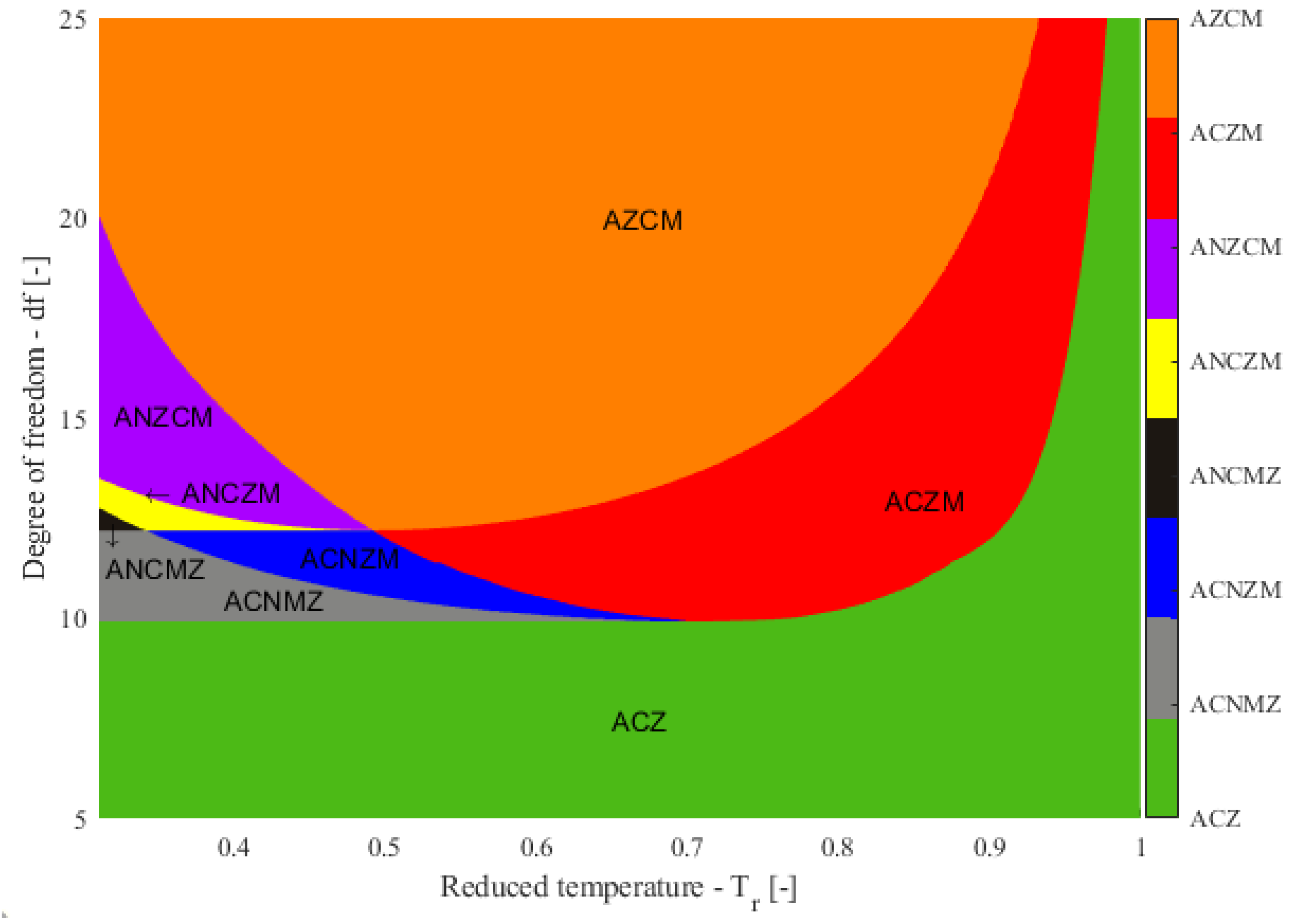In the given model, the degree of freedom was assumed to be temperature-independent; hence, molar isochoric heat capacity was taken as $c_{Vm}=\frac{df}{2}R$ [5]. Then, primary and secondary points were determined numerically using a self-made MATLAB code. Finally, using the entropy values of these points, classes were determined and plotted in a reduced temperature–degree of freedom diagram. The relevant part of the diagram (molecular degrees of freedom values between 5 and 25) is shown in Figure 4, while a magnified part, showing special points of the map, is shown in Figure 5.

All the eight classes can be found on the map (Figure 4), although some of them (like ACZ or AZCM) cover bigger areas, while others, like ANCMZ (small black triangle-shaped area) cover only a smaller portion. Some of the classes are neighboring ones, which means that by changing the temperature or molecular complexity by a small fraction, a fluid can step from one class to another (like ACZM and ACZ). Going back to butane (Figure 2), taking a lower end-point of 398.51 K, the system is emulating ACZM-type, while taking this temperature as 398.53 K, the type turns to ACZ. Other classes are more distinct, for example, from ACZM (red) it is impossible to reach ANCMZ (black) by a small step.

Borders can be divided into five, or rather four and a half parts. Two of these border lines are linear (straight line), at a fixed degree of freedom (df = 9.92 and df = 12.19). Two (and a half) others are curved ones; the first runs between green and red then blue and red, finally between violet and orange; this curve has another branch (taken as a half curve) going out from the minimum of the previous curve, separating the grey and blue, then the yellow and black regions. The first part of the border is already known and describes the location of N and M points; it has a minimum, existing even for real materials, which can be used as a rule of thumb to distinguish between wet and non-wet working fluids, based on their measured molar isochoric heat capacity in a given (fixed-value) reduced temperature [14,24]. Although there are several rules of thumb to predict at least the basic properties of working fluids, most of them are not accurate or very complex. Only a handful of them work with nearly 100% accuracy, predicting the wetness/dryness of the fluid [24,25,26] by using simple quantities for these correlations. The last line is also a curved one, running between the red-orange and the yellow-violet regions. Straight borders terminate when reaching any of the curved ones; these common points are the minima of the curved ones. Correlations (polynomial fits) of these borders can be found in Appendix B.

There are three special points on the map, where four or five classes meet; they are numbered in Figure 5, which is a magnification of the relevant part of Figure 4, showing these multiple points.

In point 1, ACZM, ACNMZ, ACNZM, and ACZ classes form a quadruple point (although ACNMZ, the grey one, seems to be terminated earlier, this is only due to numerical noise). In the immediate vicinity of this point (marked by 1 in Figure 5) one can find four different classes. It is possible to move from ACZM (red) to ACNMZ (grey) by changing the molecular complexity, characterized here by the molecular degree of freedom (df) while keeping the reduced temperature constant in a two-step or in a direct, one-step process. During a two-step process, from the ACZM (red) class, one has to reach the ACNZM class (blue) first; this happens when T(N)—the temperature of point N—which was originally hidden below the lower temperature limit, related to the solid-liquid-vapor triple-point temperature, suddenly pops up to the accessible temperature range. During the second step, from this ACNZM (blue) class, by further changing the molecular complexity, one can reach the ACNMZ class (grey); this occurs when the entropies for M and Z (s(M) and s(Z)) switch places. This happens when the so-called ideal gas-part contribution [5] increases which increasing df and shifts point M to higher entropy values. Based on the analysis of this two-step process, one can easily describe what happens during the one-step process of ACZM (red) to ACNMZ (grey). Put simply, the two independent phenomena, namely the appearance of point M (when T(N) reaches T(Z)) and the switch of M and Z (when s(Z) goes above s(M)), happen in the same place in the df–T_r space. Similar coincidences are responsible for the other quadruple point (marked as 3 in Figure 5) as well as for the existence of the quintuple point where five classes can exist within the immediate vicinity of point 2 (Figure 5).

The locations of the multiple points shown in Figure 4 and Figure 5 are shown in

Table 2. The location of the multiple points shown in Figure 5.

Point	Location
1	df = 9.92 Tr = 0.6991–0.6739
2	df = 12.19 Tr = 0.4903–0.4918
3	df = 12.19, Tr = 0.406–0.3412

, giving their reduced temperature and molecular degree of freedom coordinates.

3. Discussion: Explanation of Various Phenomena with the Map

We investigated some of our previous findings on the map. First, as we already stated, all classes turn to ACZ when the new end-point is sufficiently close to the critical point. The critical point is represented here by T_r = 1, and it is clearly seen that close to this value, only the ACZ (green) class exists.

Second, we were able to find only six classes among real materials (when the lower end-point is fixed to the triple point, around T_r = 0.3–0.4) as well as for van der Waals fluids (where we fixed the end-point to T_r = 0.3). It can be seen, that at T_r = 0.3, there are only six classes, ACZ (green), ACNMZ (grey), ANCMZ (black), ANCZM (yellow), ANZCM (violet), and finally, AZCM (orange). Also, one can see that by fixing the temperature elsewhere (for example at T_r = 0.4), we would see a similar, but not the same sequence: ANCMZ (black) would be replaced by ACNZM (blue). Fixing the end-point temperature around T_r = 0.55, the sequence would be shorter, ACZ–ACNMZ–ACNZM–ACZM–AZCM, while at an even higher temperature (T_r = 0.8), it would be a three-step process, ACZ–ACZM–AZCM.

As was seen previously, the classes found among real materials were identical with the classes found for van der Waals fluids with the end-point fixed at T_r = 0.3, but since this value has nothing to do with real triple-point temperatures (except for when using the soft rule of thumb mentioned above), we believe that this exact equality is just a lucky coincidence. However, it can still show that no more than six classes can exist when the lower end-point is fixed in a given reduced temperature.

Third, by fixing the molecular degree of freedom (i.e., taking one, fixed material) and by changing the end-point temperature from the real, triple point related one up to the critical point, the maximal number of classes emulated during this process is six (see the longer route for Figure 3). In Figure 4, by choosing a degree of freedom value around 12.5 one can see an ANCMZ (black) – ANCZM (yellow) – ANZCM (violet) – AZCM (orange) – ACZM (red) – ACZ (green), six-step sequence, while even slightly below this value, at df = 12, one can see the four-step sequence, namely ACNMZ (grey) – ACNZM (blue) – ACZM (red) – ACZ (green), down to df = 9.92. Below this value, only ACZ-type fluids exist. With more complex molecules (above df = 20) one can see only dry or wet ones (AZCM-ACZM-ACZ) for T_r > 0.3. The two lines separating the map into these regions are the straight-line borders at df = 9.92 and df = 12.19.

Fourth, as can be seen in Figure 3, three of the eight classes seem to be archetypes: ACZ, ANCMZ, and ACNMZ, the three classes at the end of this graph. ACZ occupies the high-temperature end, i.e., approaching T_r = 1, where all fluids turn to ACZ-type. On the other end, going to T_r = 0, fluids with df ≤ 9.92 (small molecules) are ACZ-type (green) and fluids with 9.92 ≤ df ≤ 12.19 (medium-size molecules) are ACNMZ-type (grey). One can assume that the black region runs up (like the green region on the high-temperature side), and therefore at the low-temperature limit, all fluids with df > 12.19 (longer molecules) would be class ANCMZ. In this way, T_r = 1 and T_r = 0 limits would be occupied only by these three archetypes.

One might ask that if the calculations for van der Waals fluids were started at a more reduced temperature (like T_r = 0.4), would the black ANCMZ region disappear? Would it not be possible to find hidden ninth or even tenth working fluid classes in temperature or degree of freedom regions not shown in Figure 4? The answer is no; it has been shown in reference [12] that these are the only classes; the existence of other classes are theoretically impossible. On the other hand, one cannot rule out that any of these eight classes could re-appear in another T_r–df region (most probably on the high-df region, representing very complex molecules), i.e., the existence of two separate regions with the same type (i.e., two distinct blue regions) cannot be fully ruled out. This problem might require further study.

It can be assumed that using other equations of states, the map can differ to some extent; these differences can be qualitative or quantitative. According to some previous results [17], the classes are probably located in a similar order when the Redlich–Kwong equation is used, but the whole diagram is shifted to higher df values. Further studies to describe these differences are in progress.

4. Conclusions and Summary

For the organic Rankine cycle, the selection of working fluid is crucial; it can affect not only the output (efficiency, power) but also the layout of the equipment used for the realization of the cycle [5,27]; this is especially true for the selection of the expander [28]. For some fluids, one may use only a basic layout of pump-evaporator-expander-condenser, while for other fluids, the use of extra parts, like a droplet separator, superheater, or recuperative heat exchanger may be necessary. The type of the layout can be correlated with the shape of the temperature–specific entropy (T–s) diagram of the given working fluid, more specifically with the shape (and location) of the saturated vapor branch of this curve. Based on the shape, one can divide existing as well as potential working fluids into various classes. The traditional three-class (wet-dry-isentropic) classification is not sufficient, because several materials can remain unclassified or misclassified, while materials listed in the same class might show crucial differences. Therefore, recently, a more detailed, eight-class classification was proposed; this new classification is compatible with the traditional ones, but can solve the problems associated with traditional ones.

Classes can be handled as material properties, using the full fluid part of the T–s diagrams (from triple point to critical point). Sometimes the lower limit (triple point) is located in temperatures hardly used in ORC processes; therefore, one shall also define a lower end-point temperature classification when the end-point of the saturated liquid and vapor branches are taken in a temperature value more practical than triple-point temperature. In the new, limited temperature range (new end-point to critical point) a working fluid belonging to a given class can emulate the general properties of another class.

Using a model fluid (like van der Waals fluid), material property can also be a smoothly changeable property, where transitions from one to another class can be demonstrated; this can help us to design novel working fluids.

In this paper, we give the map of a van der Waals fluid in a reduced temperature vs. molecular degree of freedom diagram. All the eight novel classes can be located on the map; peculiarities (for example, the fact that from real fluids we were not able to find examples for two of these classes; or, the existence of two temperature-dependent classification routes) can be easily explained using the map. Three multiple points (where more than two classes meet in a given reduced temperature and molecular degree of freedom value) were located. Although the map based on the van der Waals equation of state cannot give quantitatively correct predictions, qualitatively it can describe all known phenomena.