Optimal Management of the Energy Flows of Interconnected Residential Users

Abstract

In recent years, residential users have begun to be equipped with micro-CHP (combined heat and power) generation technologies with the aim of decreasing primary energy consumption and reducing environmental impact. In these systems, the prime mover supplies both thermal and electrical energy, and an auxiliary boiler and the national electrical grid are employed as supplementary systems. In this paper, a simulation model, which accounts for component efficiency and energy balance, was developed to replicate the interaction between the users and the energy systems in order to minimize primary energy consumption. The simulation model identified the optimal operation strategy of two residential users by investigating different energy system configurations by means of a dynamic programming algorithm. The reference scenario was compared to three different scenarios by considering independent energy systems, shared thermal and electrical energy storage and also the shared prime mover. Such a comparison allowed the identification of the most suitable energy system configuration and optimized operation strategy. The results demonstrate that the optimized operation strategy smoothes the influence of the size of thermal and electrical energy storage. Moreover, the saving of primary energy consumption can be as high as 5.1%. The analysis of the economic feasibility reveals that the investment cost of the prime mover can be as high as 4000 €/kW.

1. Introduction

1.1. Problem Statement

In recent years, several studies have focused on alternative energy production systems with the aim of reducing emissions and primary energy consumption with a target of 20% in the EU by 2020 [1], thus tackling climate change based on the 2030 Agenda for Sustainable Development [2] and the EU climate and energy framework [3]. One option to achieve these goals envisions that sustainable energy policies are implemented by rationalizing the use of energy resources [4]. The exploitation of district energy systems and smart grids also contributes to this goal.

District energy systems allow heating and cooling demand to be fulfilled [5]. In this case, the energy system is defined and/or designed for process decentralization, allowing improvements in energy efficiency by reducing carbon employment and enhancing renewable resource exploitation [6]. As stated by De Pascali and Bagaini, combined heat and power (CHP) systems represent a suitable technology that can be embedded in a district energy system; in fact, this technology can make district energy systems independent of centralized power grids [7]. In addition, onsite electricity can be provided by reducing transmission losses. Finally, waste heat can also be exploited locally [8] and pollutant emissions significantly reduced by means of flue gas treatments [9].

Unlike district energy systems, smart grids are mainly aimed at efficiently providing electricity from the sources to the end-user [10]. In the literature, different smart grid definitions exist, as discussed, for instance, in [11,12]. In general, a smart grid represents every practice or technology that can provide economic and environmental improvement to the power grid [12]. In a smart grid, energy users, called “prosumers,” can produce, consume, store or share energy with other users and the national grid.

The smart grid concept can be implemented in several ways, but, according to Ferrari et al. [12], the adoption of CHP units is one of the most promising solutions. In fact, thanks to their economic and functional advantages, CHP systems represent an attractive alternative to the separated production of heat and electricity, proving to successfully meet energy demands for both the industrial sector and residential buildings. Moreover, the study [13] clearly demonstrates that the local environmental impact of the CHP production can be significantly reduced compared to the separated production.

1.2. Literature Review

In the literature, CHP systems are described as having already been widely employed in industrial scenarios, while the residential sector presents a high penetration potential [14,15,16,17]. In fact, currently, most residential users still employ a domestic boiler and the national grid to meet their thermal and electrical energy demand, respectively. As stated in [18], building heating accounts for 40% of total energy consumption [19]. Thus, CHP units are a potential alternative to enhance primary energy savings in residential applications [20]. In the “CHP scenario,” a prime mover (PM) supplies both thermal and electrical energy. Some micro-CHP systems for residential building applications are examined in [1,4,14,21,22,23] by also considering their economic performance.

Energy management systems (EMSs) are fundamental in order to solve energy management problems [24]. In the last few years, several EMS approaches were investigated. For example, Shayeghi et al. [25] classified EMSs as (i) nonrenewable based, (ii) energy storage system based, (iii) demand-side management based and (iv) hybrid system based. Instead, Dehghanpour et al. [26] identified three different categories, namely centralized, distributed and hybrid control. Finally, Ghiani et al. [27] classified EMSs into (i) classical and exact, (ii) heuristic and metaheuristic and (iii) artificial intelligent solution. An indepth analysis was provided by Georgilakis [28]. The exploitation of EMSs has been the object of several research activities. For example, an artificial neural network provided encouraging results in [29] by significantly reducing the primary energy consumption, emissions and operating costs of a microgeneration system coupled with renewable energy. A similar energy system and objective function were optimized by Roy et al. in [30]. Artificial neural network effectiveness was also shown by Seo et al. [31]. Instead, Wang et al. [32] and Wu et al. [33] exploited particle swarm algorithms to optimize the capacity of hybrid energy storage systems.

In [34,35,36,37,38], the optimization procedure was performed by means of a mixed-integer and linear programming strategy (MILP). In particular, the papers [34,35] addressed the optimization of a domestic micro-cogeneration system and a cogeneration power plant, respectively, while distributed energy resources were optimized in [36] to minimize energy costs. Instead, Steen et al. [37] applied the MILP approach to evaluate the feasibility of combining a thermal energy storage (TES) system with distributed energy resources. Wouters et al. [38] employed a MILP model to evaluate the integration of distributed generation units and microgrids in the current grid infrastructure and identify its optimal design. The latest updates about EMSs are documented in [39,40,41]. In particular, Ford et al. [39] highlighted that there is a lack of understanding of how users interact. Rafique et al. [40] identified the optimal scheduling of electrical and gas energy resources for a smart home by using a genetic algorithm. Sanguinetti et al. [41] investigated the energy benefits related to smart home technology. Instead, Allegrini et al. [42] reviewed the tools that address district-level energy systems by focusing on district-level interactions.

Dynamic programming (DP) [43] is an optimization strategy that provides the global minimum of a given objective function. According to Yu et al. [44], DP is more effective than linear and nonlinear programming and proves its effectiveness by solving multiple objective function problems by dividing the complex problem into interrelated subproblems [44,45]. In addition, Chen et al. [46] stated that the lack of empirical coefficients and predetermined parameters constitute one of the main advantages in using DP. Nevertheless, DP may require higher computational time than linear algorithms [47], especially if the number of variables increases [46]. Thus, DP may not be suitable for online applications.

In the energy system area, several studies [46,48,49,50] proved the effectiveness of DP also for residential user applications. In [46], DP was applied to a biofuel micro-CHP system supplied with battery banks and supercapacitors, in order to identify the optimal power distribution for CHP suppliers. The study [48] also validated DP by selecting the optimal control strategy for minimizing primary energy consumption. Furthermore, DP was used in [49] to investigate the dispatch problem by considering a micro-CHP system based on a gas turbine. The DP algorithm was used in [50] to identify the operating logic that allowed cost minimization of a system, including an internal combustion engine, a boiler and a water tank with a resistor. Recently, Bahlawan et al. [51] exploited the DP algorithm in order to optimize both the sizing and operation of hybrid energy plants, with the goal of minimizing primary energy consumption.

1.3. Objective and Novelty of This Paper

This paper aims at merging the main achievements of the studies currently available in the literature in this area by combining two novel features, i.e., i) the presence of an energy grid that connects two residential users (the energy grid is considered “smart” since it is assumed bidirectional and perfectly controlled and metered) and ii) the optimization of the management strategy for different energy system configurations and component size, in order to minimize primary energy consumption.

Compared to other studies available in the literature, different perspectives make this paper unique. In fact, the DP algorithm is employed to identify the optimal operating strategy. Thus, the auxiliary boiler (AB) and the national electrical grid are always available to the users. Moreover, different sizes of both the TES and electrical energy storage (EES) are considered and the influence of the district heating grid (DHG) is analyzed. Finally, with respect to a previous study carried out by the same authors in [52], a higher number of energy system configurations are evaluated and the case study, which includes two residential users, is different. In addition, the current paper comprises and discusses the operating strategy of the optimal energy system configuration identified by the DP algorithm.

Thus, the results reported in this paper can be used to evaluate the profitability of micro-CHP systems employed for residential users, thanks to the optimized operation strategy and fine-tuned coupling of their components.

In this paper, two residential users provided the basis to analyze different arrangements of the grid and the consequent optimized operation strategy of the PMs. Four energy system configurations were evaluated and discussed: (1) reference scenario, (2) independent energy systems, (3) shared thermal and electrical energy storage and (4) shared storages and prime mover. In the “reference scenario,” a domestic AB was used for meeting thermal energy demand, while the national electrical grid (EG) supplied electrical energy. In the “independent energy systems” configuration, each of the two residential users was equipped with its own independent energy system, which was composed of a PM, a TES, an EES and an AB. Both residential users were connected with the national electrical grid and were also connected with each other by means of a local DHG. In the configuration named “shared TES and EES,” each user could exploit its own PM, AB and the connection to the EG. This means that one TES and one EES were shared between the two users. Finally, the “shared TES, EES and PM” configuration considered shared TES and EES, but the demand of both users was met by means of only one shared PM.

The simulation model optimizes the operation strategy of the PMs in order to minimize the primary energy required to meet both the thermal and electrical energy demands. The energy demands are derived from published data and reproduce a winter day of a typical residential user.

The paper is organized as follows. Section 2 presents and discusses the modeling approach and the optimization strategy. Section 3 presents the case study and the system configurations. Section 4 reports the results in terms of primary energy consumption, PM working hours and thermal and electrical energy share. Section 4 also includes a feasibility analysis and a discussion about their mutual interaction and consequent effect on PM operation strategy. Finally, conclusions and guidelines are drawn.

2. Methodology

The energy system configurations evaluated in this paper account for three main components, namely PM, TES and EES. ABs and EG are also available by providing a backup system aimed at energy fulfillment. Both the PM and the backup systems meet electrical and thermal energy demands; in addition, in case of need, thermal energy can also be supplied by a DHG.

In this paper, the most suitable strategy to switch on/off the ABs or the PM (either alternatively or simultaneously) was identified by means of the optimization algorithm discussed in Section 2.3, to minimize primary energy consumption.

2.1. Energy System Modeling

As shown in Equation (1), the state of charge (SOC) of a TES at time point (t + 1) depends on the SOC at the previous time point, i.e., t, and the thermal power P_TES entering or leaving the TES. In addition, a thermal leakage rate, defined as in [37], is included to account for thermal leakages.

$${\mathit{SOC}}_{\mathrm{TES}}^{t+1}=\left(1-{\in }_{\mathrm{th}}\right)·\left({\mathit{SOC}}_{\mathrm{TES}}^t{-P}_{\mathrm{TES}}·\Delta t\right)$$

(1)

The thermal power P_TES is calculated by means of Equation (2):

$$P_{\mathrm{TES}}={\displaystyle {\displaystyle \sum }_{\mathrm{i}=1}^{n_{\mathrm{user}}}}\left(P_{\mathrm{th},\mathrm{user},\mathrm{i}}-u_{\mathrm{i}}·P_{\mathrm{th},\max ,\mathrm{i}}-P_{\mathrm{th},\mathrm{AB},\mathrm{i}}{\pm P}_{\mathrm{th},\mathrm{DHG},\mathrm{i}}\right)$$

(2)

where P_TES, i.e., the thermal power that enters or leaves the TES, depends on the thermal demand of the user (P_th,user,i), the thermal power provided by the PM (P_th,max,i), the ABs (P_th,AB,i) and the DHG (P_th,DHG,i), which can be either entering or leaving. It is worth noting that P_th,DHG,i is null in the reference scenario, since the DHG is not included.

The SOC of each EES is estimated using Equation (3) by neglecting electrical energy leakages:

$${\mathit{SOC}}_{\mathrm{EES}}^{t+1}=\left({\mathit{SOC}}_{\mathrm{EES}}^t{-P}_{\mathrm{EES}}·\Delta t\right)$$

(3)

The electric power entering or leaving the EES (P_EES) is calculated by means of Equation (4), which accounts for inverter efficiency (η_inv) and EES charging efficiency (η_ch).

$$P_{\mathrm{EES}}=\{\begin{array}{c}{\eta }_{\mathrm{inv}}·\left({\displaystyle {\displaystyle \sum }_{\mathrm{i}=1}^{n_{\mathrm{user}}}}{P}_{\mathrm{el},\mathrm{user},\mathrm{i}}{-u}_{\mathrm{i}}·P_{\mathrm{el},\max ,\mathrm{i}}{-P}_{\mathrm{el},\mathrm{EG},\mathrm{i}}^{+}\right)\mathrm{if}{\displaystyle {\displaystyle \sum }_{\mathrm{i}=1}^{n_{\mathrm{user}}}}{P}_{\mathrm{el},\mathrm{user},\mathrm{i}}{-u}_{\mathrm{i}}·P_{\mathrm{el},\max ,\mathrm{i}}{-P}_{\mathrm{el},\mathrm{EG},\mathrm{i}}^{+}>0\\ {\eta }_{\mathrm{inv}}{\eta }_{\mathrm{ch}}·\left({\displaystyle {\displaystyle \sum }_{\mathrm{i}=1}^{n_{\mathrm{user}}}}{P}_{\mathrm{el},\mathrm{user},\mathrm{i}}{-u}_{\mathrm{i}}·P_{\mathrm{el},\max ,\mathrm{i}}{-P}_{\mathrm{el},\mathrm{EG},\mathrm{i}}^{+}\right)\mathrm{if}{\displaystyle {\displaystyle \sum }_{\mathrm{i}=1}^{n_{\mathrm{user}}}}{P}_{\mathrm{el},\mathrm{user},\mathrm{i}}{-u}_{\mathrm{i}}·P_{\mathrm{el},\max ,\mathrm{i}}{-P}_{\mathrm{el},\mathrm{EG},\mathrm{i}}^{+}\le 0\end{array}$$

(4)

If the two conditions reported in Equation (5a) are satisfied,

$$\{\begin{array}{c}{\mathit{SOC}}_{\mathrm{EES}}{=\mathit{SOC}}_{\mathrm{EES},\max }\\ {\displaystyle {\displaystyle \sum }_{\mathrm{i}=1}^{n_{\mathrm{user}}}}{P}_{\mathrm{el},\mathrm{user},\mathrm{i}}{-u}_{\mathrm{i}}·P_{\mathrm{el},\max ,\mathrm{i}}{-P}_{\mathrm{el},\mathrm{EG},\mathrm{i}}^{+}<0\end{array}$$

(5a)

then the excess of electrical energy produced by the PM is sent to the EG, as given in Equation (5b), by assuming that any excess of energy can be accepted by the national EG. It is worth noting that this assumption is justified by the fact that most EU countries favor the electricity generated by means of CHP units and priority dispatching.

$$E_{\mathrm{el},\mathrm{EG}}^{-}=\left(u·P_{\mathrm{el},\max }-P_{\mathrm{el},\mathrm{user}}\right)·\Delta t$$

(5b)

2.2. Objective Function

Primary energy consumption E_p, defined in Equation (6), accounts for the primary energy required by all the available PMs, ABs and EG to meet both thermal and electrical energy demand.

$$E_{\mathrm{p}}=\left({\displaystyle {\displaystyle \sum }_{\mathrm{i}=1}^{n_{\mathrm{PM}}}}\frac{u_{\mathrm{i}}·P_{\mathrm{el},\max ,\mathrm{i}}}{{\eta }_{\mathrm{PM},\mathrm{i}}{(u}_{\mathrm{i}})}+\frac{P_{\mathrm{th},\mathrm{AB},\mathrm{i}}}{{\eta }_{\mathrm{AB},\mathrm{i}}}+\frac{P_{\mathrm{el},\mathrm{EG},\mathrm{i}}}{{\eta }_{\mathrm{EGm}}·p}\right)·\Delta t$$

(6)

As can be seen in Equation (6), primary energy consumption depends on the electrical and thermal efficiency of the PMs, ABs and EG. More in detail, the electrical efficiency of each PM (η_PM,i) depends on its load u_i, which usually ranges from 0% to 100% (i.e., design point). The AB efficiency (η_AB,i) is selected by considering a standard non-condensing unit (see Section 3).

The primary energy employed to produce electricity in the national electrical grid depends on its efficiency η_EGm (this is a mean value, depending on the considered country and generation technologies) and grid losses, by means of the parameter p that also depends on the considered country.

2.3. Optimization Algorithm

As previously mentioned, this study makes use of DP [43], to identify the absolute minimum of a given objective function, as well as meeting user-defined constraints. A DP model, which is a sequential decision process, is characterized by states and decisions. The former, i.e., the “state,” provides a picture of the situation at a given time point by allowing the evaluation of alternative courses of action. The latter, i.e., the “decision” also called “control variable”, is an action that modifies the state, until a final state is achieved.

The alternating sequence of states and decisions constitutes the path through the state space. The DP algorithm requires a discrete and static time model of the systems. In fact, DP works backward; the algorithm starts from the final time point and goes back until the initial time point is reached.

Benefits of the DP algorithm were reported in several research papers, for example, [53]. With respect to other optimization strategies, DP is generally exploited thanks to (i) its efficiency, (ii) its independence from the linearity or nonlinearity of the problem and (iii) its capability to identify a solution that represents the global optimum.

The control variables and states considered in this paper are listed in

Table 1. Control variables and states.

Energy System Component	Variable	DP (Dynamic Programming) Component
PM (prime mover)	u	Control variable
AB (auxiliary boiler)	Pth,AB	Control variable
DHG (district heating grid)	Pth,DHG	Control variable
EG (electrical grid)	Pel,EG	Control variable
TES (thermal energy storage)	SOCTES	State
EES (electrical energy storage)	SOCEES	State

. The control variables were four, i.e., one per each component. All the possible combinations of values of these control variables were analyzed across the selected time frame, to achieve the minimization of the objective function (in this paper, overall primary energy consumption). Instead, the two states were the SOCs of the TES and the EES. It is worth noting that an increase of the number of states makes the computational time increase exponentially and thus modeling efforts are usually made to reduce its number.

All the analyses carried out in this paper were performed in the Matlab^® environment. In particular, the DP algorithm was implemented based on the routine developed by [54] and available at [55].

3. Case Study

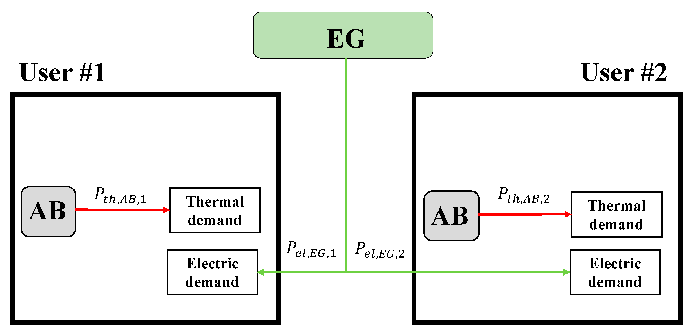
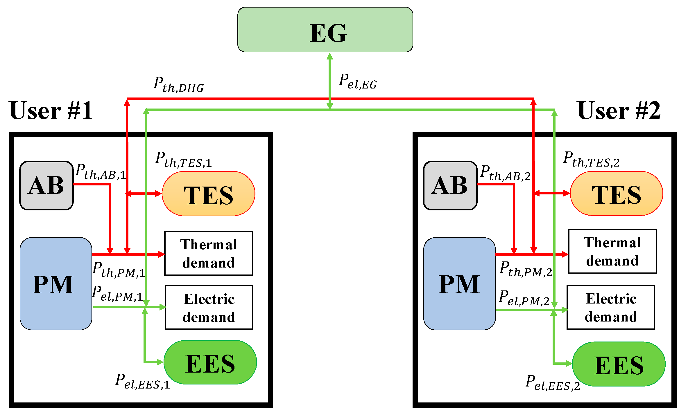
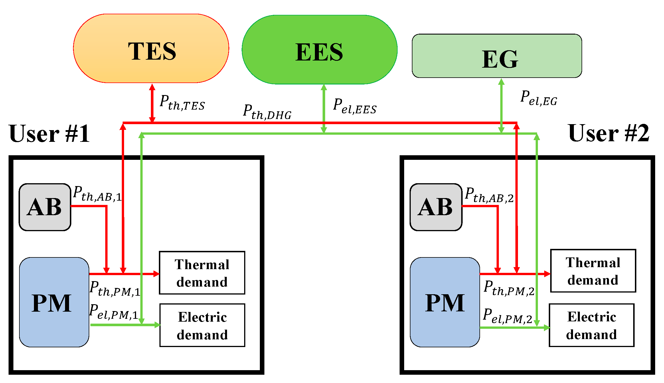
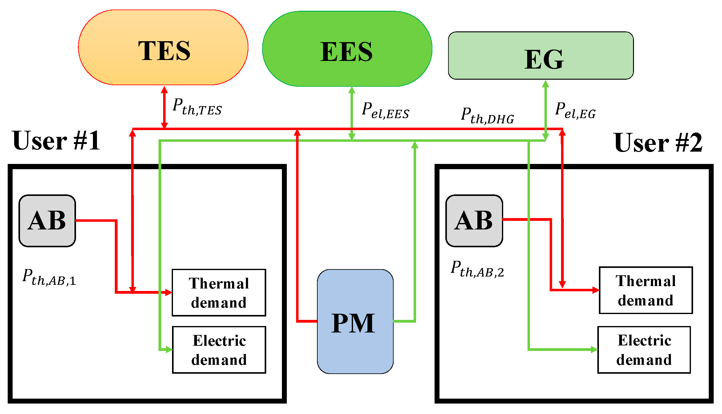
3.1. Energy System Configuration

The case study considered two residential users. Four configurations, i.e., (1) reference scenario, (2) independent energy systems, (3) shared TES and EES and (4) shared TES, EES and PM, were analyzed. Thus, with respect to Cattozzo et al. [52], the “independent energy systems” scenario was also investigated in this paper.

“Reference scenario”. In the “reference scenario”, sketched in Figure 1, thermal energy demand was met by an AB (one for each user), while electrical energy demand was supplied by the EG.

“Independent energy systems”. Figure 2 shows the “independent energy systems” configuration, in which each of the two residential users was equipped with its own independent energy system. Each energy system was composed of a PM, a TES, an EES and an AB. Both residential users were connected with the national EG and were also connected with each other by means of a local DHG.

“Shared TES and EES”. The “shared TES and EES” configuration accounts for one AB and one PM for each user (see Figure 3). In addition, each user was connected to the national EG. Thus, in this case, the storages were shared by the users.

“Shared TES, EES and PM”. This configuration, namely “shared TES, EES and PM”, aimed at peak shaving between the users and was consequently expected to increase the number of PM working hours. In fact, in this configuration (see Figure 4), one PM was shared by the two users to meet their energy demand.

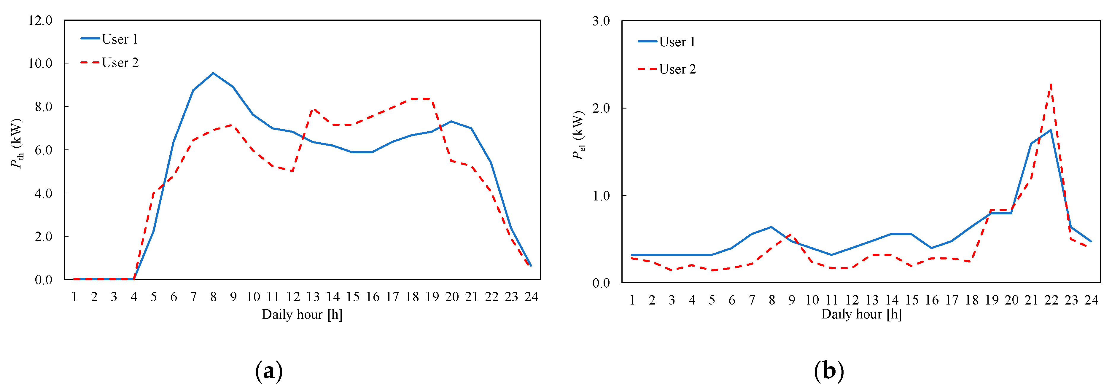
3.2. User Energy Demand

The thermal and electrical energy demands required by both residential users, i.e., user 1 and user 2, are sketched in Figure 5a,b. These trends, which were also used in [52], refer to a typical winter day. In particular, the energy demand required by user 1 was derived by [56], while the energy demand of user 2 was obtained by imposing small random variations on the demand of the user 1. In this manner, the two energy demands were slightly different, but comparable. The same trend of the user 1 was also used in [14] for evaluating the capability of micro-CHP systems to meet the household energy demands of single-family users and in [57] for analyzing the transient behavior of micro-CHP systems.

In any case, it must be highlighted that the overall results presented in Section 4 do not depend on the number of considered users, since they just scale if more users are modeled.

3.3. Prime Mover

Because of their current market availability [57,58,59,60], even for low electric power outputs (as low as 1 kW [14]), the PM was an internal combustion engine, named Honda Ecowill. The nominal values of electric and thermal power outputs and efficiencies are reported in

Table 2. Prime mover nominal performance.

PM	Pel (kW)	Pth (kW)	ηel	ηth	Ref.
Honda Ecowill	1.00	3.25	0.200	0.630	[14]

for the considered engine. The electric power output is equal to 1 kW. In this paper, PM load modulation was not allowed, i.e., only two operation modes were possible for the PM, i.e., no load or full load.

It must be also highlighted that, when multiple PMs were considered for meeting a given demand (scenarios “Independent energy systems” and “Shared TES and EES”), the PMs were of the same type.

3.4. Electrical and Thermal Energy Storage

The capacity of the TES and EES is a key factor to optimize CHP system operation and meet a given energy demand in an effective way, as well as the proper sizing and scheduling of storage systems heavily affect their application [61]. For this reason, a sensitivity analysis was performed on both the TES and EES capacities for the “independent energy systems” configuration, in order to evaluate the respective optimal size. The TES sizes (10 and 15 kWh) and EES sizes (2.5 and 5.0 kWh) were selected in agreement with the users’ energy demand and by evaluating similar applications reported in [62].

Instead, in the “shared TES and EES” and “shared TES, EES and PM” configurations the sensitivity analysis was not carried out and the sizes were assumed equal to twice the optimal TES and EES sizes identified for the “independent energy systems” configuration.

3.5. System Parameters

The system parameters reported in

Table 3. Constant model parameters.

Efficiency	Value	Reference
ηAB	0.900	[63]
ηEG	0.460	[64]
p	0.851	[63]
ηinv	0.94	[65]
ηch	0.98	Assumption

are assumed constant. In fact, in practice, they cannot be optimized by the user, but are driven by standards (e.g., η_AB and p) or depend on the national grid (i.e., η_EGm). Finally, the two efficiencies η_inv and η_ch are usually very high and thus their variation negligibly influence the results.

3.6. Control Variables and States

The range of discretization and variation of the control variables and states are reported in

Table 4. Control variables and states.

Energy System Component	Variable	Minimum Value	Maximum Value	Discretization
PM	u	0	1	Binary value
AB	Pth,AB	0 kW	24 kW	5 steps
DHG	Pth,DHG	−Pth,user,max	+Pth,user,max	5 steps
EG	Pel,EG	0	+Pel,user,max	5 steps
TES	SOCTES	5% SOCTES,max	95% SOCTES,max	Continuous
EES	SOCEES	5% SOCEES,max	95% SOCEES,max	Continuous

. The assumptions made are discussed as follows.

The load u can only be 0, i.e., the PM is not working, or 1, i.e., the PM works at nominal load. The nominal thermal power of the AB is 24 kW, which is a typical value for household applications [14,18,29]. The maximum thermal power exchanged through the DHG does not exceed the PM nominal power output. Finally, the electrical energy supplied by the national grid is equal to the maximum electrical energy demand of the user, at maximum.

It is clear that an infinitely fine discretization of the control variables can lead to the most optimized result. However, this also makes the computational cost increase dramatically, since DP solver is particularly time consuming. Therefore, as a trade-off between accuracy and computational time, five discrete values are considered for the AB, DHG and EG control variables.

The two states SOC_TES and SOC_EES, which are the output of the DP algorithm, are identified by means of a continuous function that ranges from 5% to 95% of the TES and EES nominal capacity. In such a manner, the TES and EES cannot be completely charged and discharged taking into accounted their actual technical limits.

Finally, by considering real-world operation of internal combustion reciprocating engines, the minimum switch-on time frame of the PM was assumed equal to 30 minutes.

4. Results

The simulated period was selected to be a working week composed of six identical winter days, of which the energy demand is shown in Figure 5. Another reason for selecting such a timeframe is that SOC relative variation across the considered time frame is lower than 1.5% for all the analyzed configuration and component sizes.

The analyses carried out in this paper were aimed at evaluating (i) primary energy consumption, (ii) PM working hours, (iii) thermal and electrical energy share and (iv) optimal operation strategy identified by the DP algorithm, which allows the minimization of the primary energy consumption.

Finally, it must be considered that in the three scenarios that consider the presence of at least one PM (i.e., all the scenarios with the exception of the reference scenarios), electrical energy could be delivered to the EG (see Equation (5b)). For this reason, the primary energy used to produce such electricity was added to the electrical energy produced in the corresponding reference scenario. Thus, the production of useful energy (electrical and thermal) was exactly the same and primary energy consumption values could be coherently compared.

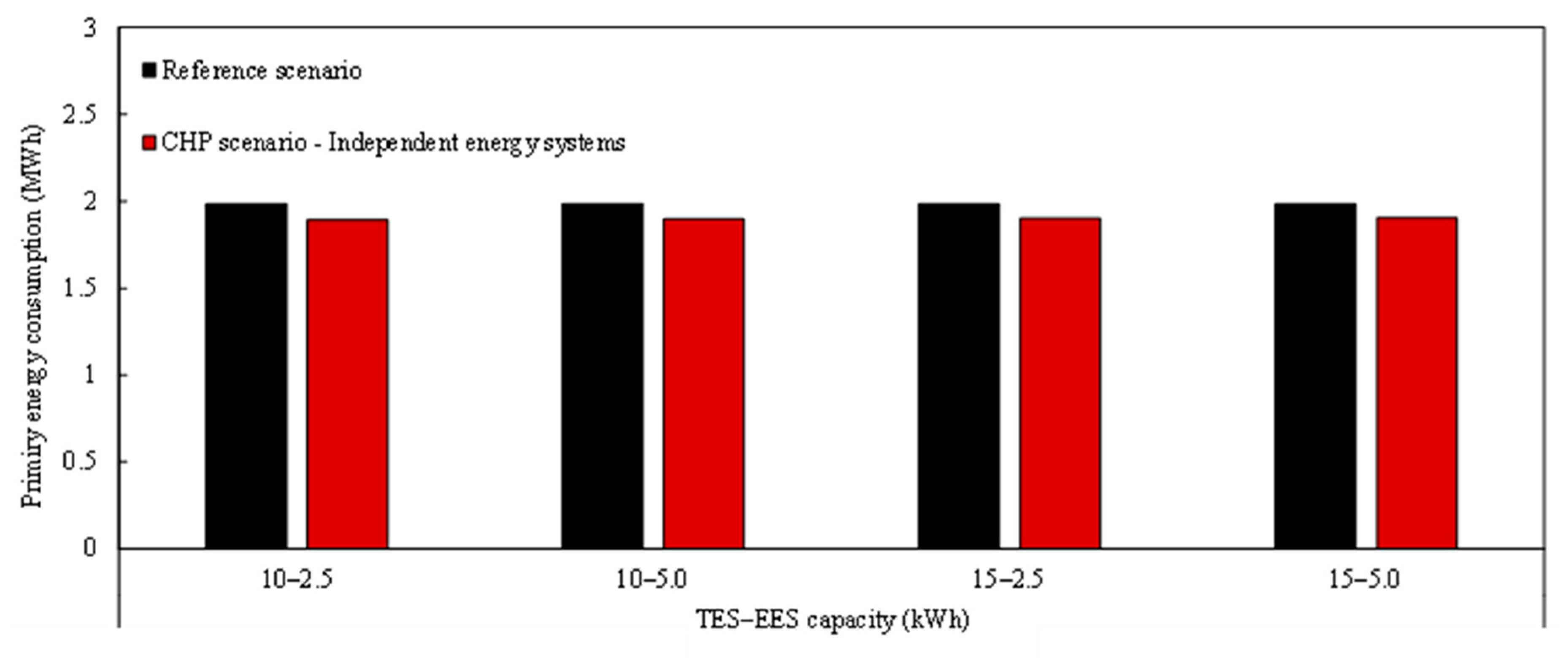
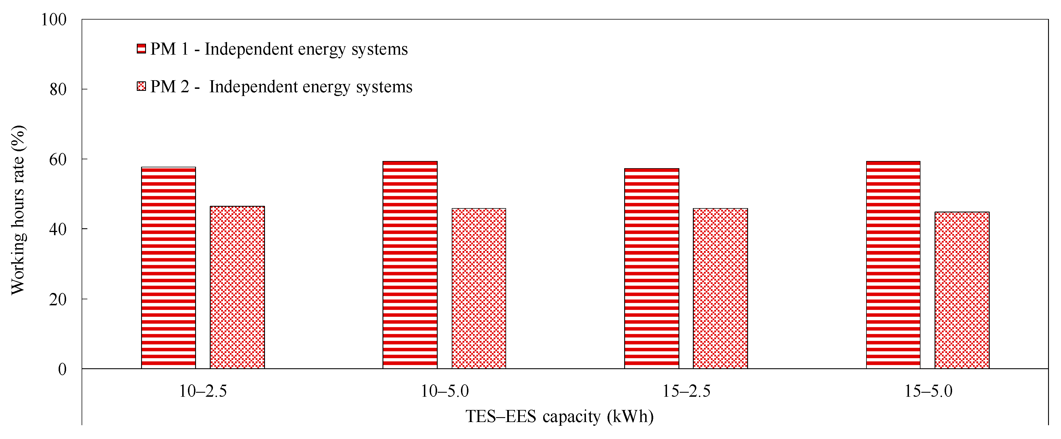
4.1. Primary Energy Consumption and PM Working Hours

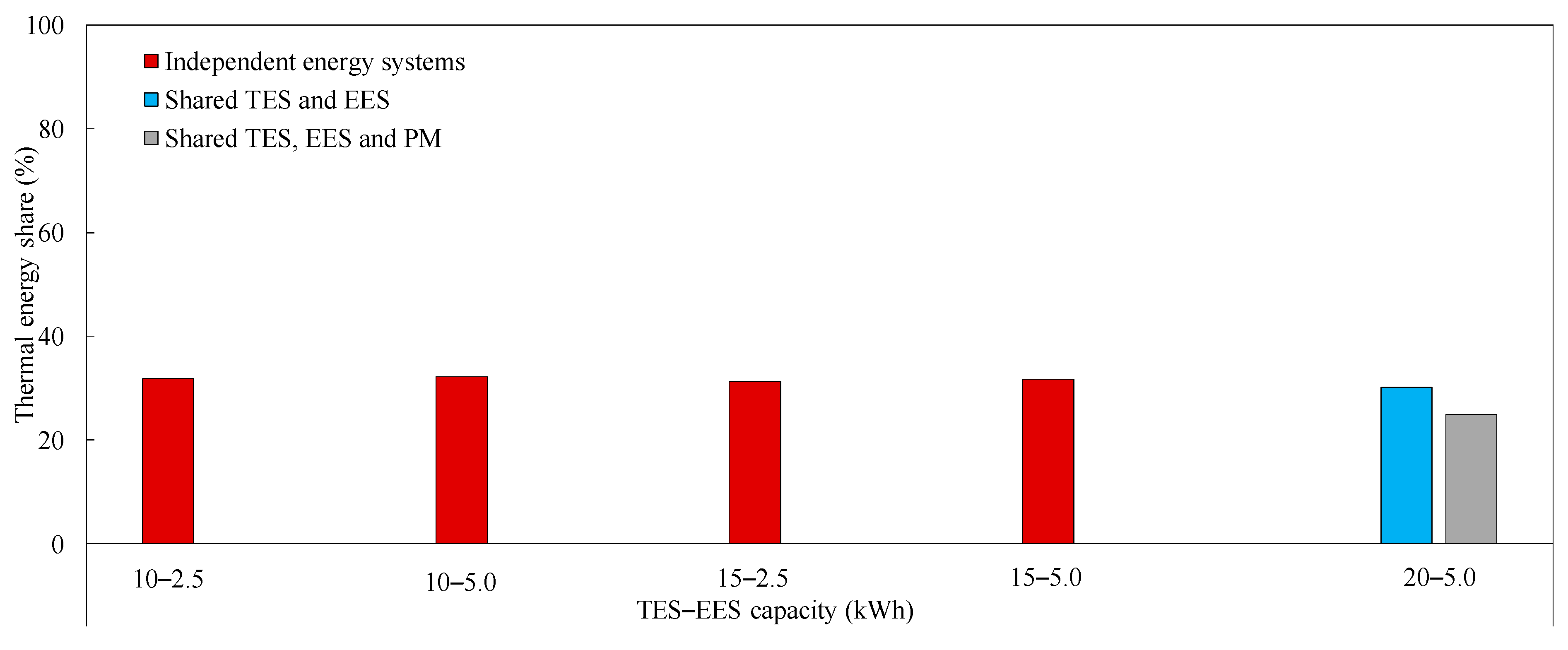
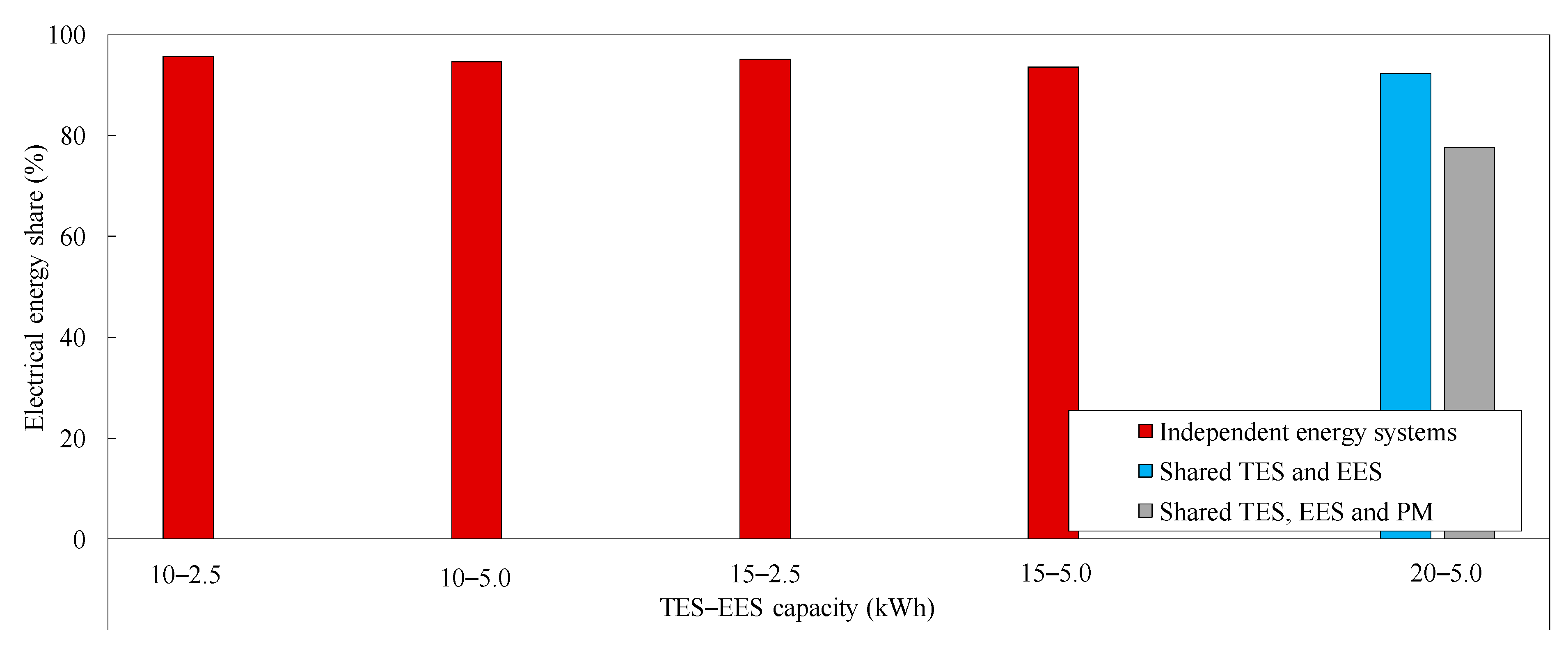
“Independent energy systems”. As outlined in Figure 6, the primary energy consumption related to the CHP scenario was slightly dependent on TES and EES sizes. Compared to the “reference scenario”, the primary energy consumption saved by means of the independent energy system configuration ranged from 3.9% (with the highest TES and EES capacity values) to 4.6% (with the lowest TES and EES capacity values).

Figure 7 shows the rate of PM working hours (defined as the ratio of the number of working hours and the maximum number of working hours during six days) corresponding to the primary energy consumption values reported in Figure 6. The rate of PM working hours confirms to be quite unaffected by TES and EES sizes. Therefore, the TES and EES of minimum capacities (10 and 2.5 kWh, respectively) proved to be the optimal solution both in terms of primary energy consumption (1.89 MWh) and PM working hours (58% for PM 1 and 47% for PM 2, see

Table 5. Primary energy consumption and rate of PM working hours.

	Reference Scenario	CHP Scenario
		“Independent energy systems” (TES: 10 kWh; EES: 2.5 kWh)	“Shared TES and EES” (TES: 20 kWh; EES: 5 kWh)	“Shared TES, EES and PM” (TES: 20 kWh; EES: 5 kWh)
Primary energy consumption	1.98 MWh	1.89 MWh	1.88 MWh	1.91 MWh
Rate of PM working hours	N/A	58% (PM 1) 47% (PM 2)	64% (PM 1) 26% (PM 2)	81% (shared PM)

).

“Shared TES, EES and PM”. Table 5 reports both the primary energy consumption and rate of PM working hours associated with the “shared TES and EES” and “shared TES, EES and PM” configurations with only one TES and EES size (20 and 5 kWh, respectively) assumed to be twice the optimal capacities identified in the “independent energy systems” configuration. The primary energy saving compared to the “reference scenario” was equal to 5.1% if each user was equipped with one PM (“shared TES and EES configuration”). In this configuration, the rate of working hours was equal to 64% for PM 1, whereas it was equal to 26% for PM 2. Instead, in the “shared TES, EES and PM configuration,” the energy saving was equal to 3.7% and the shared PM ran for 81% of the considered timeframe.

4.2. Energy Share

The values of thermal and electrical energy share are reported in Figure 8 and Figure 9, respectively. These figures also highlight the influence of the energy system configuration and storage sizing.

Regardless of system configuration, the thermal energy share covered by the PMs was generally in the range 25–32% (see Figure 8). Thus, the remaining thermal energy demand had to be provided by the ABs.

Instead, as shown in Figure 9, the PMs met most of the electrical energy demand. Thus, the energy systems were generally self-sufficient, i.e., independent of the EG.

The analysis of the results reported in Figure 6 through Figure 9 and in Table 5 highlights that two energy system configurations were generally preferable: (i) “shared TES and EES,” equipped with two Ecowill PMs and (ii) “shared TES, EES and PM,” equipped with one Ecowill PM. These solutions represent the best configurations since they allowed almost the same primary energy consumption, but the PM ran longer than in the case of the “independent energy system” configuration and, in addition, the PM met most of the electrical energy demand. Moreover, it must be noted that primary energy consumption and working hours were slightly affected by TES and EES capacities, regardless of the considered energy system configuration.

4.3. Optimized Strategy

This paragraph reports an insight about the optimized strategies of the most suitable energy system configurations, i.e., (i) “shared TES and EES” and (ii) “shared TES, EES and PM”. In both cases, the TES and EES capacities were the same, i.e., 20 and 5 kWh, respectively. More in detail, the PM and AB working conditions, the TES and EES state of charge and the power energy taken from and delivered to the national electrical grid are discussed. Figure 10 and Figure 11 show the optimized strategies across six days for comparison purposes.

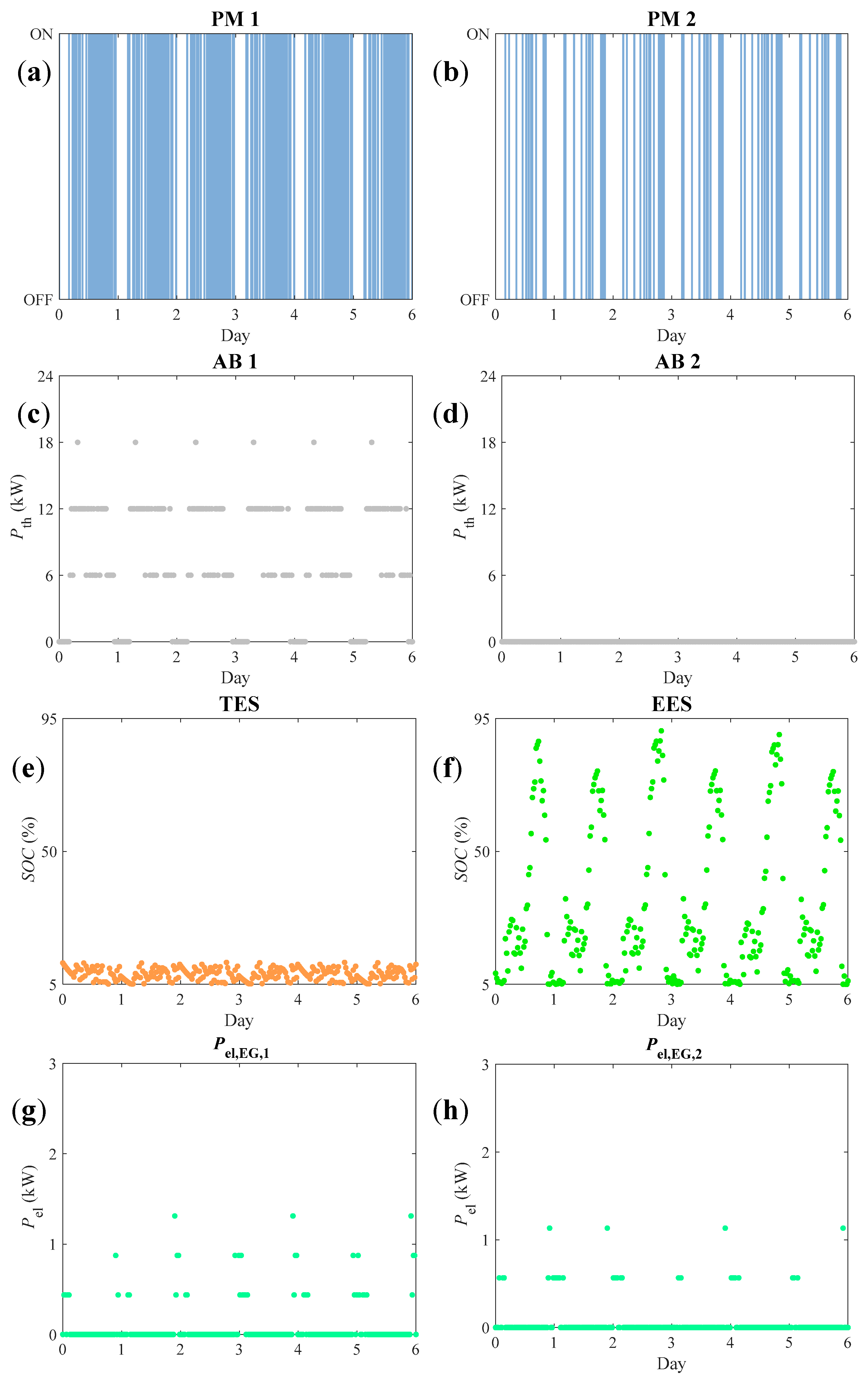
4.3.1. Optimized Strategy with Shared TES and EES

The “shared TES and EES” configuration which required the lowest primary energy consumption involved the following parameters:

• 2 Ecowill PMs;
• TES capacity, 20 kWh;
• EES capacity, 5.0 kWh.

In Figure 10a,b, the bar plots titled “PM 1” and “PM 2” show the switch-on time of the two PMs. It is worth noting that both PMs worked for a significant amount of hours, even if, as highlighted in Table 5, PM 1 covered most of the energy demand, while PM 2 generally worked for peak-shaving purposes. The two figures labeled “AB 1” and “AB 2” (Figure 10c,d) show the thermal power supplied by the ABs. As can be seen, the maximum thermal power (24 kW) was never supplied. In fact, AB 1 supplied at maximum 18 kW in correspondence of the maximum thermal power demand, while AB 2 was always switched off. As a result, the TES (Figure 10e) seems to be oversized since its SOC was always lower than 15%. Instead, the SOC of EES (Figure 10f) reached the maximum value of 91%.

By comparing the SOC of the EES and the electric power taken from the national electrical grid (see Figure 10g,h), it is evident that both users usually needed electric power from the national electrical grid at the same time points, i.e., when the SOC of the EES was at a minimum. In fact, electrical energy was taken from the grid, but it was never delivered to the grid.

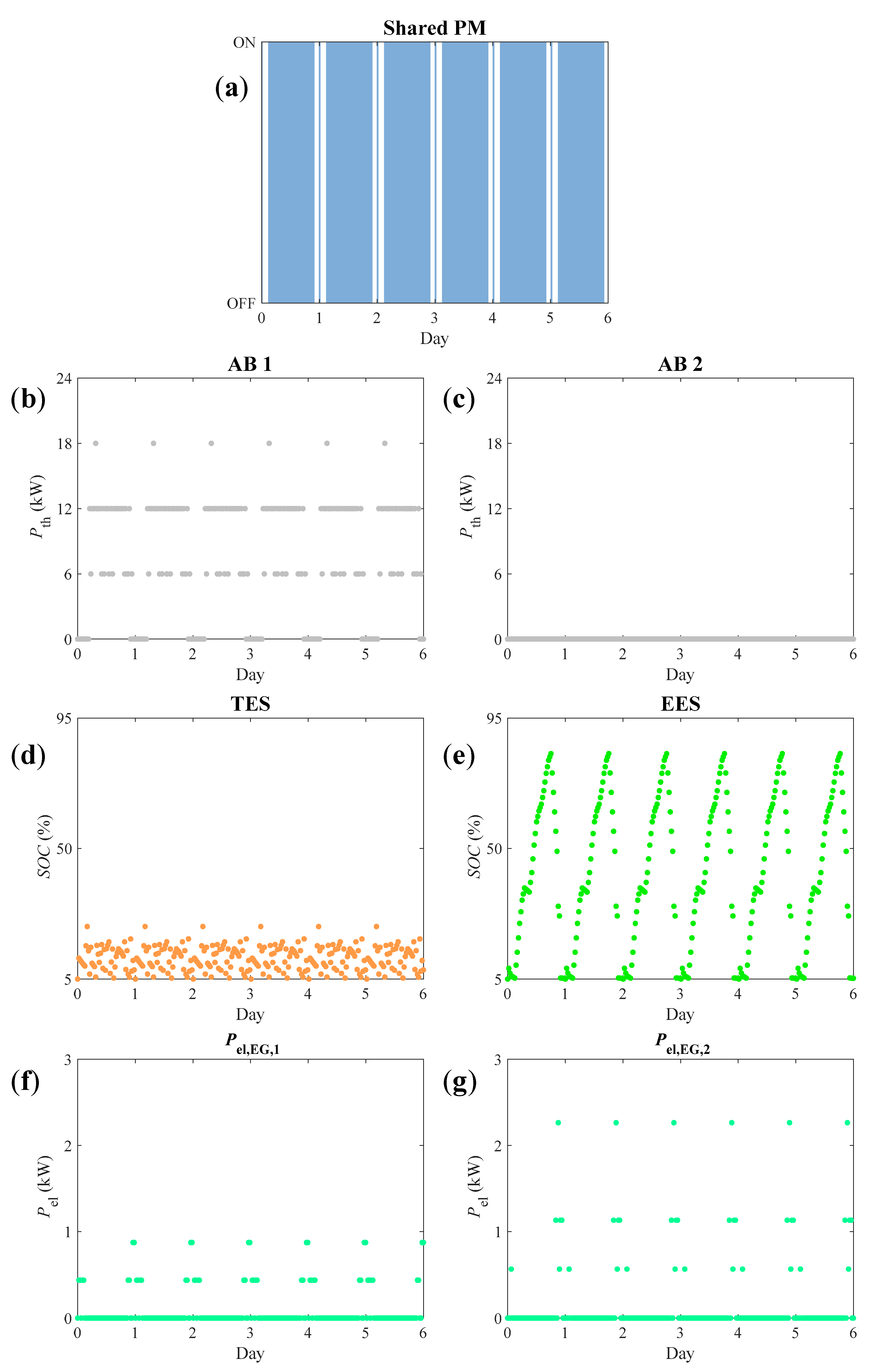
4.3.2. Optimized Strategy with Shared TES, EES and PM

The details of the operation of the best optimized strategy with “shared TES, EES and PM” are reported in Figure 11. The CHP configuration included:

• 1 Ecowill PM;
• TES capacity, 20 kWh;
• EES capacity, 5.0 kWh.

In agreement with the results shown in Table 5, Figure 11a confirms that the shared PM worked almost all the day, with the exception of the beginning of the day (when only electric power was required) and the end of the day (when thermal and electrical energy was very low).

The daily thermal energy profile which was supplied by AB 1 was coherent with the thermal energy demand of the users; in fact, as sketched in Figure 11b, AB 1 started working as soon as the thermal energy was required and the maximum thermal power, i.e., 18 kW, was supplied when the thermal peak demand occurred. On the contrary, AB 2 never worked (Figure 11c). Thus, since the AB nominal power (i.e., 24 kW) was never supplied, AB 1 was oversized and AB 2 was redundant. As noted for the previous configuration, the TES capacity was significantly oversized; in fact, its maximum SOC was always lower than 25% (see Figure 11d). Instead, the SOC of the EES increased over time, with its maximum at roughly 80% (Figure 11e). Finally, both users had to take electrical energy from the national electrical grid (Figure 11f,g), both when the PM was switched off and at the end of the day. In fact, the PM and EES did not completely meet the power demand. As a result, the energy system never delivered electric power to the national electrical grid.

4.4. Discussion

The comprehensive analysis of Figure 6, Figure 7, Figure 8, Figure 9, Figure 10 and Figure 11 and Table 5 allows the identification of the most suitable energy system configuration by integrating different pieces of information.

By comparing the two optimized strategies, it is clear that the thermal power supplied by AB 1 in both configurations was roughly the same. Moreover, in both cases AB 2 was redundant and TES and EES were always oversized since their maximum capacity was never exploited. As a result, the energy system configuration could be further simplified by sharing one AB and reducing the TES and EES sizes. Thus, the primary energy consumption would not vary, but the energy system installation costs can be reduced.

If both the TES and the EES were shared by the two residential users, the saving was increased to 5.1%, while, if the PM was also shared, the saving with respect to the “reference scenario” dropped to 3.7%, but the cost of one PM could be avoided. It should be noted that the saving of primary energy consumption was affected by the low size of the CHP system (1 kWe) used, characterized by low electrical and thermal efficiency values (20% and 63%, respectively). Moreover, it should also be noted that other studies document a comparable decrease of primary energy consumption [48,52,66].

4.5. Economic Feasibility

This section evaluates the economic feasibility of the two most suitable energy system configurations (“shared TES and EES” and “shared TES, EES and PM”) by considering the respective optimized strategy (see Section 4.3.), i.e., the one that allowed the lowest primary energy consumption. The economic feasibility of these two configurations is compared to that of the “reference scenario”.

In the “reference scenario”, the costs considered are the investment and maintenance cost of the ABs, the purchase cost of natural gas used to feed the ABs and electricity purchase cost.

Instead, in the “shared TES and EES” and “shared TES, EES and PM” configurations, the following investment costs are attributed to system components:

• one or two PMs (two PMs in the “shared TES and EES” configuration, one PM in the “shared TES, EES and PM” configuration);
• one AB (in fact, as shown in Figure 10 and Figure 11, one of the two ABs was always switched off);
• one TES;
• one EES.

For the investment costs, a straight-line amortization over 10 years is considered by assuming that amortization costs are charged only over the winter period (180 days), while the discount rate is assumed equal to 5%.

Maintenance costs are accounted for in the following system components:

• one or two PMs (see the comment above),
• one AB (see the comment above),
• one TES.

Instead, the maintenance cost of the EES is neglected, according to [67].

Moreover, for the “shared TES and EES” and “shared TES, EES and PM” configurations, natural gas purchase cost and electricity purchase cost are also included as required in the “reference scenario,” while it must be noted that electrical energy is not delivered to the national electrical grid and thus the possible corresponding revenue is null.

The purchase cost of electricity and natural gas assumed in this analysis refers to the Italian market in the first week of 2019 for households and varies on an hourly basis. In such a week, the hourly specific overall cost varied from 115.0 to 177.3 €/MWh, with an average value of 154.6 €/MWh. The cost of natural gas is assumed constant and equal to 0.23 €/Sm³, in line with the Italian natural gas market.

Table 6. Assumptions for the feasibility analysis.

Energy System Component	Investment Cost	Maintenance Cost
PM	Estimated	22.5 €/MWh [68]
AB	100 €/kW	2% of investment cost [69]
TES	10 €/kWh [70]	50 €/year [71]
EES	171 €/kWh [67] or 844 €/kWh [67]	0 [67]

summarizes the assumptions made for carrying out the feasibility analysis. It should be noted that two different EES technologies [67], i.e., lead–acid battery (171 €/kWh) or Li–ion battery (844 €/kWh), are considered. Moreover, it must be highlighted that the investment cost of the PM is estimated as a trade-off value which renders the yearly cash flow of the two “shared TES and EES” and “shared TES, EES and PM” configurations equal to the yearly cash flow in the “reference scenario.” Therefore, such a value represents the maximum allowable investment cost of the PM to make the two “shared TES and EES” and “shared TES, EES and PM” configurations economically equivalent with respect to the “reference scenario.” Otherwise, incentives should be provided to make the PM investment cost affordable.

Table 7. Trade-off value of the investment cost of the PM.

System Configuration	Lead–Acid Battery (171 €/kWh)	Li–Ion Battery (844 €/kWh)
Shared TES and EES	2000 €/kW	300 €/kW
Shared TES, EES and PM	4000 €/kW	450 €/kW

reports the trade-off value of the investment cost of the PM for the two considered configurations and two EES technologies.

If a lead–acid battery is employed, the PM investment cost should be lower than 2000 €/kW for the “shared TES and EES” configuration, whereas it is doubled if the “shared TES, EES and PM” configuration is considered. Instead, if a Li–ion battery is considered, the PM investment cost should be lower than 450 €/kW.

However, as sketched in Figure 10 and Figure 11 and discussed in Section 4.4, the shared TES is oversized. Thus, TES capacity may be even halved. However, such a solution does not significantly affect the results, since the maximum allowable investment cost of the PM would be increased by 100 €/kW at maximum.

The economic viability of micro-CHP systems used in residential applications may be further improved by considering that several configurations investigated in this paper allow electrical energy to be delivered to the national electrical grid. Several recent studies investigated the potential synergy between micro-CHP systems and electric vehicle charging. The profitability of micro-CHP systems is thus expected to significantly improve, as demonstrated in [72,73], also thanks to optimized strategies and algorithms for smart charging control systems [74]. Moreover, incentives can be provided to make micro-CHP technologies more attractive.

5. Conclusions

This paper compared different configurations of micro-CHP systems and different sizing of both TES and EES, in order to minimize the primary energy consumption of two residential users.

One of the main outcomes of this paper is that primary energy consumption is slightly affected by the TES and EES size. This result, which differs from most studies reported in the literature, is obtained thanks to the operation strategy identified through a dynamic programming algorithm.

Another significant achievement is the quantification of the primary energy saving that can be achieved by exploiting micro-CHP technologies. The saving can be as high as 4.6% by considering the independent energy system configuration. If both the TES and the EES are shared among the two residential users, the saving is increased to 5.1%; if the PM is also shared, then the saving with respect to the reference scenario drops to 3.7%, but the cost of one PM can be avoided. Such a result was complemented with the analysis of the optimized operation strategy identified by the dynamic programming algorithm. In fact, one auxiliary boiler proved in practice useless and can be thus avoided, so that energy system installation costs are further reduced.

Finally, the economic feasibility was also evaluated with respect to the reference scenario by considering two EES technologies. Such analysis revealed that, in the most favorable case, PM investment cost can be as high as 4000 €/kW.

Future work will investigate the capability of the optimized strategy by also incorporating renewable energy technologies.

References

1. Barbieri, E.S.; Melino, F.; Morini, M. Influence of the thermal energy storage on the profitability of micro-CHP systems for residential building applications. Appl. Energy 2012, 97, 714–722. [Google Scholar] [CrossRef]
2. Transforming Our World: The 2030 Agenda for Sustainable Development, A/RES/70/1. Available online: https://sustainabledevelopment.un.org (accessed on 3 February 2020).
3. Available online: https://ec.europa.eu/clima/policies/strategies/2030_en (accessed on 3 February 2020).
4. Caliano, M.; Bianco, N.; Graditi, G.; Mongibello, L. Economic optimization of a residential micro-CHP system considering different operation strategies. Appl. Therm. Eng. 2016, 101, 592–600. [Google Scholar] [CrossRef]
5. Andersen, A.N.; Østergaard, P.A. A method for assessing support schemes promoting flexibility at district energy plants. Appl. Energy 2018, 225, 448–459. [Google Scholar] [CrossRef]
6. De Pascali, P.; Bagaini, A. Energy transition and urban planning for local development. A critical review of the evaluation of integrated spatial and energy planning. Energies 2019, 12, 35. [Google Scholar] [CrossRef] [Green Version]
7. Cho, H.; Luck, R.; Eksioglu, S.; Chamra, L.M. Cost-optimized real-time operation of CHP systems. Energy Build. 2009, 41, 445–451. [Google Scholar] [CrossRef]
8. Sameti, M.; Haghighat, F. Optimization approaches in district heating and cooling thermal network. Energy Build. 2017, 140, 121–130. [Google Scholar] [CrossRef]
9. Yin, S.; Xia, J.; Jiang, Y. Characteristics Analysis of the Heat-to-Power Ratio from the Supply and Demand Sides of Cities in Northern China. Energies 2020, 13, 242. [Google Scholar] [CrossRef] [Green Version]
10. Soares, J.; Ghazvini, M.A.F.; Vale, Z.; Oliveira, P.M. A multi-objective model for the day-ahead energy resource scheduling of a smart grid with high penetration of sensitive loads. Appl. Energy 2016, 162, 1074–1088. [Google Scholar] [CrossRef]
11. Espe, E.; Potdar, V.; Chang, J. Prosumer Communities and Relationships in Smart Grids: A Literature Review, Evolution and Future Directions. Energies 2018, 11, 2528. [Google Scholar] [CrossRef] [Green Version]
12. Ferrari, L.; Esposito, F.; Becciani, M.; Ferrara, G.; Magnani, S.; Andreini, M.; Bellissima, A.; Cantù, M.; Petretto, G.; Pentolini, M. Development of an optimization algorithm for the energy management of an industrial Smart User. Appl. Energy 2017, 208, 1468–1486. [Google Scholar] [CrossRef]
13. Bianchi, M.; Branchini, L.; De Pascale, A.; Peretto, A. Application of environmental performance assessment of CHP systems with local and global approaches. Appl. Energy 2014, 130, 774–782. [Google Scholar] [CrossRef]
14. Barbieri, E.S.; Spina, P.R.; Venturini, M. Analysis of innovative micro-CHP systems to meet household energy demands. Appl. Energy 2012, 97, 723–733. [Google Scholar] [CrossRef]
15. Raine, R.D.; Finney, K.N.; Swithenbank, J. Optimisation of combined heat and power production for buildings using heat storage. Energy Convers. Manag. 2014, 87, 164–174. [Google Scholar] [CrossRef]
16. Ghadimi, P.; Kara, S.; Kornfeld, B. The optimal selection of on-site CHP systems through integrated sizing and operational strategy. Appl. Energy 2014, 126, 38–46. [Google Scholar] [CrossRef]
17. Buoro, D.; Pinamonti, P.; Reini, M. Optimization of a Distributed Cogeneration System with solar district heating. Appl. Energy 2014, 124, 298–308. [Google Scholar] [CrossRef]
18. De Paepe, M.; D’Herdt, P.; Mertens, D. Micro-CHP systems for residential applications. Energy Convers. Manag. 2006, 47, 3435–3446. [Google Scholar] [CrossRef]
19. Reynolds, J.; Ahmad, M.W.; Rezgui, Y.; Hippolyte, J.-L. Operational supply and demand optimisation of a multi-vector district energy system using artificial neural networks and a genetic algorithm. Appl. Energy 2019, 235, 699–713. [Google Scholar] [CrossRef]
20. Brett, D.; Fraga, E.S.; Brett, D.J. A modelling study for the integration of a PEMFC micro-CHP in domestic building services design. Appl. Energy 2018, 225, 85–97. [Google Scholar]
21. Comodi, G.; Giantomassi, A.; Severini, M.; Squartini, S.; Ferracuti, F.; Fonti, A.; Cesarini, D.N.; Morodo, M.; Polonara, F. Multi-apartment residential microgrid with electrical and thermal storage devices: Experimental analysis and simulation of energy management strategies. Appl. Energy 2015, 137, 854–866. [Google Scholar] [CrossRef]
22. Orehounig, K.; Evins, R.; Dorer, V. Integration of decentralized energy systems in neighbourhoods using the energy hub approach. Appl. Energy 2015, 154, 277–289. [Google Scholar] [CrossRef]
23. McKenna, R.; Merkel, E.; Fichtner, W. Energy autonomy in residential buildings: A techno-economic model-based analysis of the scale effects. Appl. Energy 2017, 189, 800–815. [Google Scholar] [CrossRef] [Green Version]
24. Zia, M.F.; Elbouchikhi, E.; Benbouzid, M. Microgrids energy management systems: A critical review on methods, solutions, and prospects. Appl. Energy 2018, 222, 1033–1055. [Google Scholar] [CrossRef]
25. Shayeghi, H.; Shahryari, E.; Moradzadeh, M.; Siano, P. A Survey on Microgrid Energy Management Considering Flexible Energy Sources. Energies 2019, 12, 2156. [Google Scholar] [CrossRef] [Green Version]
26. Dehghanpour, K.; Colson, C.; Nehrir, H. A Survey on Smart Agent-Based Microgrids for Resilient/Self-Healing Grids. Energies 2017, 10, 620. [Google Scholar] [CrossRef]
27. Ghiani, E.; Serpi, A.; Pilloni, V.; Sias, G.; Simone, M.; Marcialis, G.L.; Armano, G.; Pegoraro, P.A. A Multidisciplinary Approach for the Development of Smart Distribution Networks. Energies 2018, 11, 2530. [Google Scholar] [CrossRef] [Green Version]
28. Georgilakis, P.S. Review of Computational Intelligence Methods for Local Energy Markets at the Power Distribution Level to Facilitate the Integration of Distributed Energy Resources: State-of-the-art and Future Research. Energies 2020, 13, 186. [Google Scholar] [CrossRef] [Green Version]
29. Entchev, E.; Yang, L.; Ghorab, M.; Rosato, A.; Sibilio, S. Energy, economic and environmental performance simulation of a hybrid renewable microgeneration system with neural network predictive control. Alex. Eng. J. 2018, 57, 455–473. [Google Scholar] [CrossRef] [Green Version]
30. Roy, K.; Mandal, K.K.; Mandal, A.C.; Patra, S.N. Analysis of energy management in micro-grid—A hybrid BFOA and ANN approach. Renew. Sustain. Energy Rev. 2018, 82, 4296–4308. [Google Scholar] [CrossRef]
31. Seo, B.; Yoon, Y.; Mun, J.; Cho, S. Application of Artificial Neural Network for the Optimum Control of HVAC Systems in Double-Skinned Office Buildings. Energies 2019, 12, 4754. [Google Scholar] [CrossRef] [Green Version]
32. Wang, H.; Wang, T.; Xie, X.; Ling, Z.; Gao, G.; Dong, X. Optimal Capacity Configuration of a Hybrid Energy Storage System for an Isolated Microgrid Using Quantum-Behaved Particle Swarm Optimization. Energies 2018, 11, 454. [Google Scholar] [CrossRef] [Green Version]
33. Wu, T.; Shi, X.; Liao, L.; Zhou, C.; Zhou, H.; Su, Y. A Capacity Configuration Control Strategy to Alleviate Power Fluctuation of Hybrid Energy Storage System Based on Improved Particle Swarm Optimization. Energies 2019, 12, 642. [Google Scholar] [CrossRef] [Green Version]
34. Collazos, A.; Maréchal, F.; Gahler, C. Predictive optimal management method for the control of polygeneration systems. Comput. Chem. Eng. 2009, 33, 1584–1592. [Google Scholar] [CrossRef]
35. Wille-Haussmann, B.; Erge, T.; Wittwer, C. Decentralized optimization of cogeneration in virtual power plants. Solar Energy 2010, 84, 604–611. [Google Scholar] [CrossRef]
36. Ren, H.; Gao, W. A MILP model for integrated plan and evaluation of distributed energy systems. Appl. Energy 2010, 87, 1001–1014. [Google Scholar] [CrossRef]
37. Steen, D.; Stadler, M.; Cardoso, G.; Groissböck, M.; Deforest, N.; Marnay, C. Modeling of thermal storage systems in MILP distributed energy resource models. Appl. Energy 2015, 137, 782–792. [Google Scholar] [CrossRef] [Green Version]
38. Wouters, C.; Fraga, E.S.; James, A. An energy integrated, multi-microgrid, MILP (mixed-integer linear programming) approach for residential distributed energy system planning—A South Australian case-study. Energy 2015, 85, 30–44. [Google Scholar] [CrossRef] [Green Version]
39. Ford, R.; Pritoni, M.; Sanguinetti, A.; Karlin, B. Categories and functionality of smart home technology for energy management. Build. Environ. 2017, 123, 543–554. [Google Scholar] [CrossRef] [Green Version]
40. Rafique, M.K.; Haider, Z.M.; Mehmood, K.K.; Zaman, M.S.U.; Irfan, M.; Khan, S.U.; Kim, C.-H. Optimal Scheduling of Hybrid Energy Resources for a Smart Home. Energies 2018, 11, 3201. [Google Scholar] [CrossRef] [Green Version]
41. Sanguinetti, A.; Karlin, B.; Ford, R.; Salmon, K.; Dombrovski, K. What’s energy management got to do with it? Exploring the role of energy management in the smart home adoption process. Energy Effic. 2018, 11, 1897–1911. [Google Scholar] [CrossRef] [Green Version]
42. Allegrini, J.; Orehounig, K.; Mavromatidis, G.; Ruesch, F.; Dorer, V.; Evins, R. A review of modelling approaches and tools for the simulation of district-scale energy systems. Renew. Sustain. Energy Rev. 2015, 52, 1391–1404. [Google Scholar] [CrossRef]
43. Bellman, R. Dynamic Programming; University Press: Princeton, NJ, USA, 1957. [Google Scholar]
44. Yu, S.; Gao, S.; Sun, H. A dynamic programming model for environmental investment decision-making in coal mining. Appl. Energy 2016, 166, 273–281. [Google Scholar] [CrossRef]
45. Seijo, S.; Del Campo, I.; Echanobe, J.; García-Sedano, J. Modeling and multi-objective optimization of a complex CHP process. Appl. Energy 2016, 161, 309–319. [Google Scholar] [CrossRef]
46. Chen, X.; Hewitt, N.; Li, Z.; Wu, Q.; Yuan, X.; Roskilly, T. Dynamic programming for optimal operation of a biofuel micro CHP-HES system. Appl. Energy 2017, 208, 132–141. [Google Scholar] [CrossRef] [Green Version]
47. Berrueta, A.; Heck, M.; Jantsch, M.; Ursúa, A.; Sanchis, P. Combined dynamic programming and region-elimination technique algorithm for optimal sizing and management of lithium-ion batteries for photovoltaic plants. Appl. Energy 2018, 228, 1–11. [Google Scholar] [CrossRef]
48. Gambarotta, A.; Morini, M.; Pompini, N.; Spina, P.R. Optimization of Load Allocation Strategy of a Multi-source Energy System by Means of Dynamic Programming. Energy Procedia 2015, 81, 30–39. [Google Scholar] [CrossRef] [Green Version]
49. Rist, J.F.; Dias, M.F.; Palman, M.; Zelazo, D.; Cukurel, B. Economic dispatch of a single micro-gas turbine under CHP operation. Appl. Energy 2017, 200, 1–18. [Google Scholar] [CrossRef]
50. Alahaivala, A.; Heß, T.; Cao, S.; Lehtonen, M. Analyzing the optimal coordination of a residential micro-CHP system with a power sink. Appl. Energy 2015, 149, 326–337. [Google Scholar] [CrossRef]
51. Bahlawan, H.; Morini, M.; Pinelli, M.; Spina, P.R. Dynamic programming based methodology for the optimization of the sizing and operation of hybrid energy plants. Appl. Therm. Eng. 2019, 160, 113967. [Google Scholar] [CrossRef]
52. Cattozzo, M.; Manservigi, L.; Spina, P.R.; Venturini, M. Minimization of the primary energy consumption of residential users connected by means of an energy grid. In Proceedings of the AIP Conference Proceedings, Modena, Italy, 11–13 September 2019; 2019; Volume 2191, p. 020041. [Google Scholar] [CrossRef]
53. Marano, V.; Rizzo, G.; Tiano, F.A. Application of dynamic programming to the optimal management of a hybrid power plant with wind turbines, photovoltaic panels and compressed air energy storage. Appl. Energy 2012, 97, 849–859. [Google Scholar] [CrossRef]
54. Sundstrom, O.; Guzzella, L. A generic dynamic programming Matlab function. In Proceedings of the 18th IEEE International Conference on Control Applications Part of 2009 IEEE Multi-Conference on Systems and Control, Saint Petersburg, Russia, 8–10 July 2009. [Google Scholar]
55. Available online: http://www.idsc.ethz.ch/research-guzzella-onder/downloads.html (accessed on 21 January 2019).
56. Macchi, E.; Campanari, S.; Silva, P. La Microcogenerazione a Gas Naturale; Polipress: Milano, Italy, 2006. [Google Scholar]
57. Ippolito, F.; Venturini, M. Development of a Simulation Model of Transient Operation of Micro-Combined Heat and Power Systems in a Microgrid. J. Eng. Gas Turbines Power 2017, 140, 032001. [Google Scholar] [CrossRef]
58. Ziviani, D.; Beyene, A.; Venturini, M. Advances and challenges in ORC systems modeling for low grade thermal energy recovery. Appl. Energy 2014, 121, 79–95. [Google Scholar] [CrossRef]
59. Adam, A.; Fraga, E.S.; Brett, D. Options for residential building services design using fuel cell based micro-CHP and the potential for heat integration. Appl. Energy 2015, 138, 685–694. [Google Scholar] [CrossRef]
60. Murugan, S.; Horák, B. A review of micro combined heat and power systems for residential applications. Renew. Sustain. Energy Rev. 2016, 64, 144–162. [Google Scholar] [CrossRef]
61. Xiong, L.; Nour, M. Nour Techno-Economic Analysis of a Residential PV-Storage Model in a Distribution Network. Energies 2019, 12, 3062. [Google Scholar] [CrossRef] [Green Version]
62. Ren, H.; Gao, W.; Ruan, Y. Optimal sizing for residential CHP system. Appl. Therm. Eng. 2008, 28, 514–523. [Google Scholar] [CrossRef]
63. COMMISSION DELEGATED REGULATION (EU) 2015/2402 of 12 October 2015, Official Journal of the European Union. Available online: https://eur-lex.europa.eu (accessed on 3 February 2020).
64. Decreto Ministeriale 5 Settembre 2011—Regime di Sostegno per la Cogenerazione ad alto Rendimento; 2011. Available online: https://www.mise.gov.it/images/stories/normativa/DM-5-SETTEMBRE2011.pdf (accessed on 3 February 2020). (In Italian)
65. Available online: https://www.e-education.psu.edu/eme812/node/738 (accessed on 3 February 2020).
66. Facci, A.L.; Ubertini, S. Analysis of a fuel cell combined heat and power plant under realistic smart management scenarios. Appl. Energy 2018, 216, 60–72. [Google Scholar] [CrossRef]
67. Telaretti, E.; Ippolito, M.G.; Dusonchet, L. A Simple Operating Strategy of Small-Scale Battery Energy Storages for Energy Arbitrage under Dynamic Pricing Tariffs. Energies 2015, 9, 12. [Google Scholar] [CrossRef] [Green Version]
68. Darrow, K.; Tidball, R.; Wang, J.; Hampson, A. Catalog of CHP Technologies, U.S. Environmental Protection Agency Combined Heat and Power Partnership; 2017. Available online: https://www.epa.gov/sites/production/files/2015-07/documents/catalog_of_chp_technologies.pdf (accessed on 3 March 2020).
69. Mapping and Analyses of the Current and Future (2020–2030) Heating/Cooling Fuel Deployment (Fossil/Renewables); European Commission Directorate-General for Energy Directorate C; 2—New Energy Technologies, Innovation and Clean Coal. 2016. Available online: https://ec.europa.eu/energy/sites/ener/files/documents/mapping-hc-excecutivesummary.pdf (accessed on 3 March 2020).
70. Sarbu, I.; Sebarchievici, C. A Comprehensive Review of Thermal Energy Storage. Sustainability 2018, 10, 191. [Google Scholar] [CrossRef] [Green Version]
71. Available online: https://www.metrotherm.dk/en (accessed on 3 March 2020).
72. Ribberink, H.; Entchev, E. Exploring the potential synergy between micro-cogeneration and electric vehicle charging. Appl. Therm. Eng. 2014, 71, 677–685. [Google Scholar] [CrossRef]
73. Angrisani, G.; Canelli, M.; Roselli, C.; Sasso, M. Integration between electric vehicle charging and micro-cogeneration system. Energy Convers. Manag. 2015, 98, 115–126. [Google Scholar] [CrossRef]
74. García-Villalobos, J.; Zamora, I.; Martin, J.I.S.; Asensio, F.J.; Aperribay, V. Plug-in electric vehicles in electric distribution networks: A review of smart charging approaches. Renew. Sustain. Energy Rev. 2014, 38, 717–731. [Google Scholar] [CrossRef]
Figure 1. Reference scenario.
Energies 13 01507 g001
Figure 2. CHP scenario with independent energy systems.
Energies 13 01507 g002
Figure 3. CHP scenario with shared TES and EES.
Energies 13 01507 g003
Figure 4. CHP scenario with shared TES, EES and PM.
Energies 13 01507 g004
Figure 5. Daily power demand of two users: (a) thermal power, (b) electric power.
Energies 13 01507 g005
Figure 6. Primary energy consumption with independent energy systems.
Energies 13 01507 g006
Figure 7. Rate of PM working hours with independent energy systems.
Energies 13 01507 g007
Figure 8. Thermal energy share.
Energies 13 01507 g008
Figure 9. Electrical energy share.
Energies 13 01507 g009
Figure 10. Best optimized strategy with “shared TES and EES”: (a) PM 1 switch-on time; (b) PM 2 switch-on time; (c) thermal power supplied by AB 1; (d) thermal power supplied by AB 2; (e) state of charge of the TES; (f) state of charge of the EES; (g) electric power taken from the electrical grid by user 1; (h) electric power taken from the electrical grid by user 2.
Energies 13 01507 g010
Figure 11. Best optimized strategy with “shared TES, EES and PM”: (a) shared PM switch-on time; (b) thermal power supplied by AB 1; (c) thermal power supplied by AB 2; (d) state of charge of the TES; (e) state of charge of the EES; (f) electric power taken from the electrical grid by user 1; (g) electric power taken from the electrical grid by user 2.
Energies 13 01507 g011