Fault Model and Travelling Wave Matching Based Single Terminal Fault Location Algorithm for T-Connection Transmission Line: A Yunnan Power Grid Study

Abstract

Due to the complex structure of the T-connection transmission lines, it is extremely difficult to identify the reflected travelling wave from the fault point and that from the connection point by the measurement from only one terminal. According to the characteristics of the structure of the T-connection transmission line, the reflection of the travelling wave within the line after the failure of different sections in T-connection transmission line are analyzed. Based on the lattice diagram of the travelling wave, the sequence of travelling waves detected at the measuring terminal varies with the fault distance and the faulty section. Moreover, the sequence of travelling waves detected in one terminal is unique at each faulty section. This article calculates the arrival time of travelling waves of fault points at different locations in different sections to form the collection of the travelling wave arrival time sequence. Then the sequence of travelling waves of the new added fault waveforms is extracted to compare with the sequences in the collection for the faulty section identification and fault location. This proposed method can accurately locate the fault with different fault types, fault resistances and system impedances by only single-terminal fault data. Both Power Systems Computer Aided Design/ Electromagnetic Transients including DC (PSCAD/EMTDC) and actual measurement data are implemented to verify the effectiveness of this method.

1. Introduction

With the global emphasis on environmental protection and the recent acceleration of urbanization, an increasing number of clean energy sources, e.g., wind turbines and photovoltaics, have been merged into the Chinese power grid through 110 kV transmission lines [1,2,3,4]. Particularly, the Yunnan power grid is the regional power grid with the highest proportion of clean energy power generation in China, which is an important power base for China’s significant national strategy of power transmission from west to east [5,6,7,8]. Therefore, 110 kV grids are the significant part of the Yunnan power grid for large-scale clean energy integration and power supply for cities [9,10,11,12]. Due to the land shortage in cities, the T-connection transmission line, which requires less area coverage and economic cost than multiple two-terminal transmission lines, is usually selected in 110 kV grids in China [13,14,15]. Moreover, the massive area coverage of mountains in Yunnan Province induces more transmission line faults, e.g., bird streamers [16], lightning [17] and gales [18]; hence, accurate fault location in the 110 kV transmission line is indeed profoundly important.

A number of fault location methods for the T-connection transmission line are available in the literature. Reference [19] proposes a fault location method by deriving the phase difference without considering the influence of distributed capacitance. Furthermore, the method of fault location based on measured impedance, which is the most popular fault location method in practice, is susceptible to the effects of fault resistance [20], fault distance [21], and system structure [22]. To determine the location of the fault point, reference [23] utilizes voltage and current signals at the three measuring terminals of the T-connection transmission line to apply a fault location method based on the distributed parameter model of the line. After the fault branch is identified in reference [24,25], the travelling wave method of the double-terminal transmission line is applied to locate the fault. [26] analyzes the time differences between the wave travelling from the connection point to the three terminals and the wave from the fault point to the three terminals. Based on this relationship, the fault branch is determined, and then the fault distance between the fault point and the three terminals is calculated [27]. The above methods are all based on the multiterminal data, which require high accuracy of communication, and GPS time sampling [28,29,30].

The method proposed in this paper does not need to identify the subsequent travelling waves of the fault points one by one, which is different from the traditional fault location method. After the fault, the initial travelling wave can be measured by a high-frequency sampling acquisition device installed in the substation. Then, the reflected travelling wave, which is from the fault point, the connection point and the other terminals, can be detected. Theoretically, a fault occurring at any point on the T-connection transmission line can induce a unique corresponding relationship of subsequently reflected travelling waves. Therefore, a set of the sequence of the travelling waves can match a specific fault distance at the faulty section. This paper discusses the characteristics of the travelling wave propagation in the T-connection transmission line to explain the relationship between the sequence of travelling waves at the measurement terminal and the location of the fault point. Secondly, the singular value information is extracted through multiple recursive singular value decomposition (SVD) transformations to obtain the sequence of travelling waves. Thirdly, the faults with different fault distance and faulty sections are applied to form the collection of the sequence of travelling waves. Then, the sequence of travelling waves of the new additional fault data is calculated to compare with the collection of sequences. Finally, the fault point is located by selecting the data of the collection which is the most similar to the new additional data.

The remainder of this paper is organized as follows: Section 2 is devoted to analysis of the travelling wave propagation characteristics of the T-connection transmission line, and of the travelling wave arrival moment sequence under different fault locations. Section 3 attempts to apply multiple recursive SVD transformations to detect the travelling wavefronts. In Section 4, simulation results are presented to verify the robustness of the proposed fault location method. Section 5 illustrates the test of a set of practical field data recorded in Yunnan province. Finally, some conclusions are summarized in Section 6.

2. Travelling Wave Propagation Characteristics of T-Connection Transmission Line

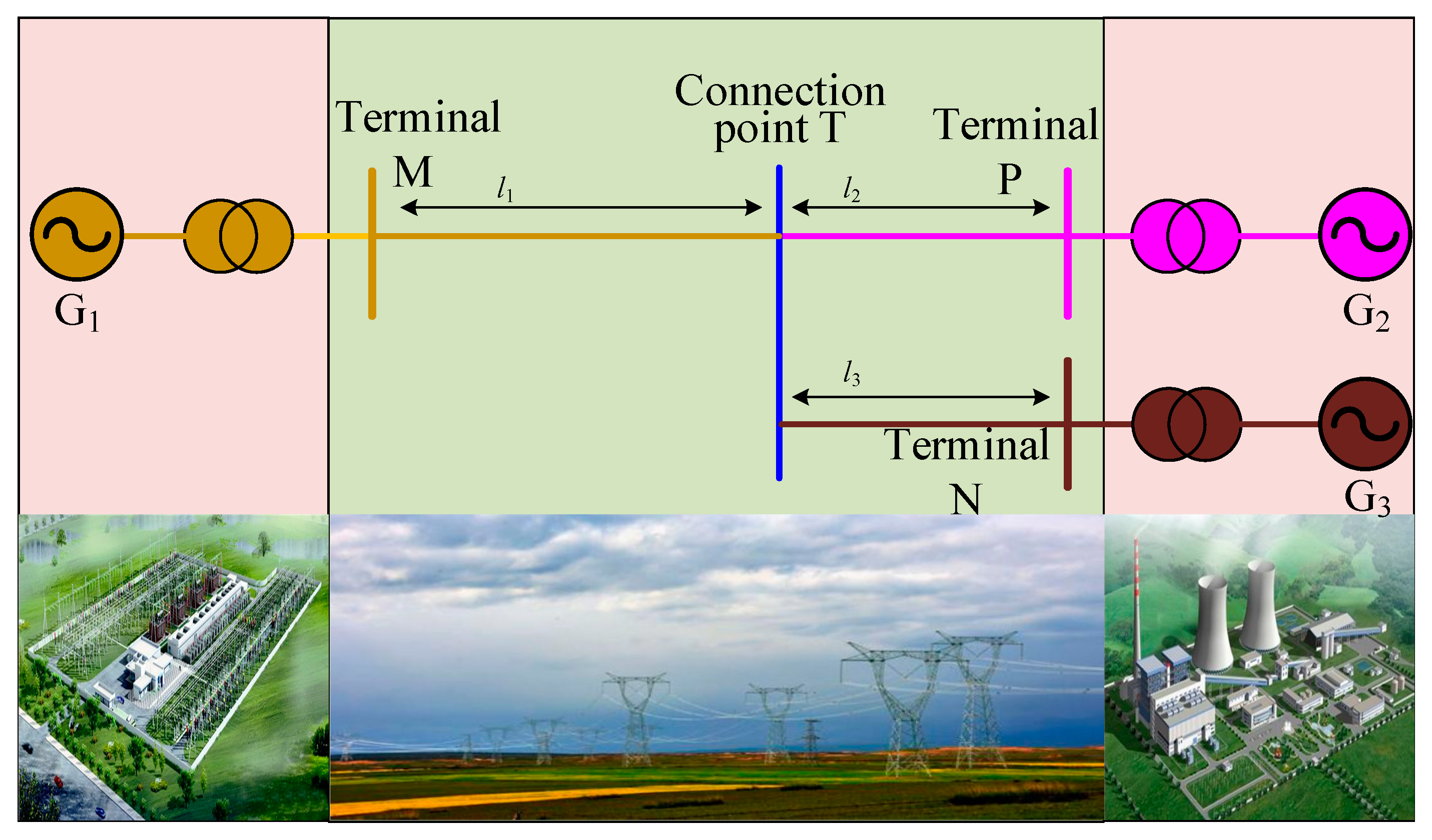
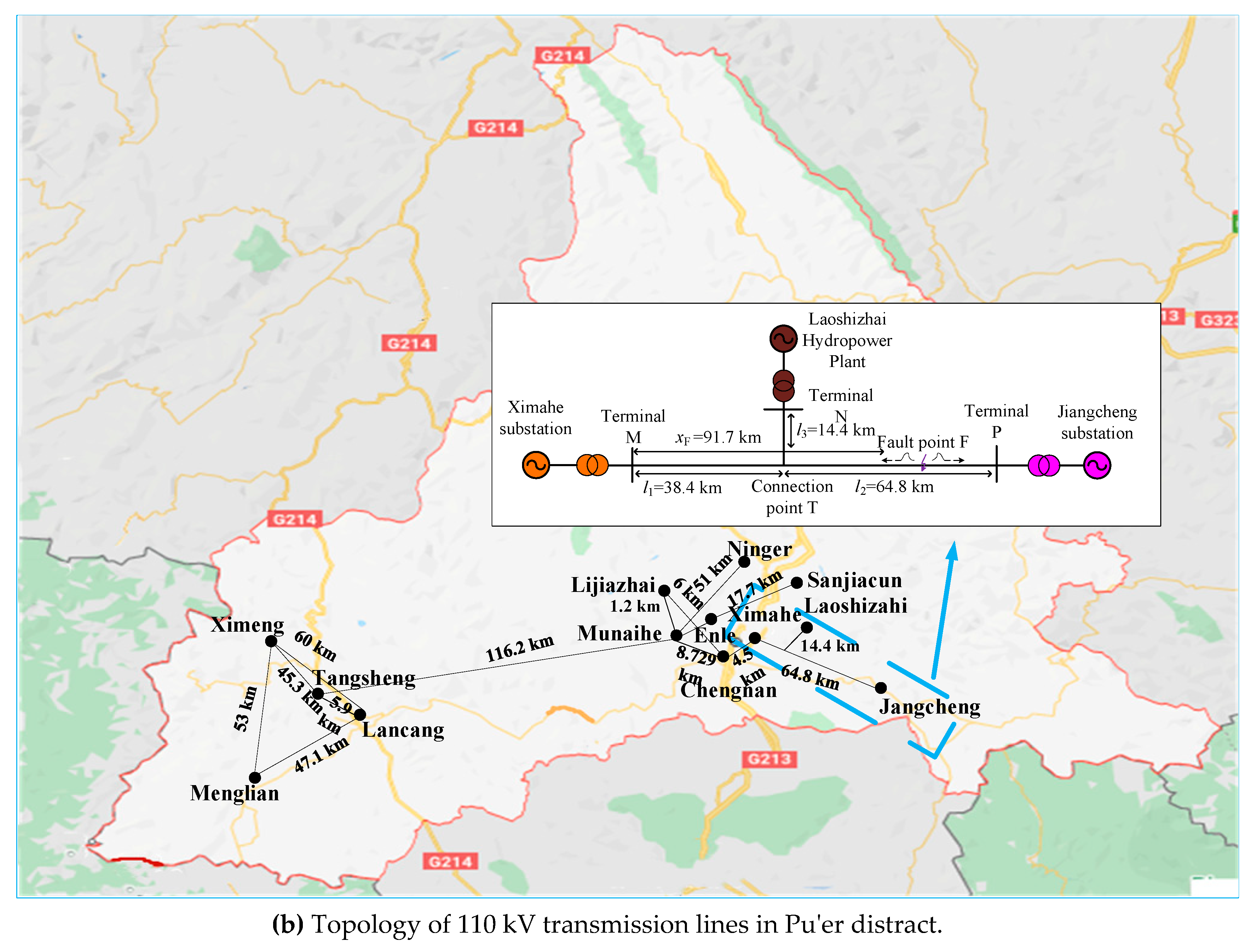
The equivalent topology of the T-connection transmission line is shown in Figure 1. M, N, and P represent the three terminals of the T-connection transmission line; T is the connection point; l₁ is the line distance from M to T; l₂ is the line distance from P to T; l₃ is the distance from N to T. In actual engineering, the lengths of the three terminals to the connection point cannot be totally identical. In order to simplify the analysis, it is assumed that l₁ > l₃ > l₂ in this paper. Terminal M is applied as the measurement terminal to discuss.

2.1. Travelling Wave Propagation Characteristics of Faults in Section MT

We assume that the distance from the fault point F to the measurement terminal M is $x_{\mathrm{F}}$, l₁ is the line distance from terminal M to connection point T, l₂ is the line distance from terminal P to connection point T, while l₃ is the distance from terminal N to connection point T, furthermore l₁ > l₃ > l₂.

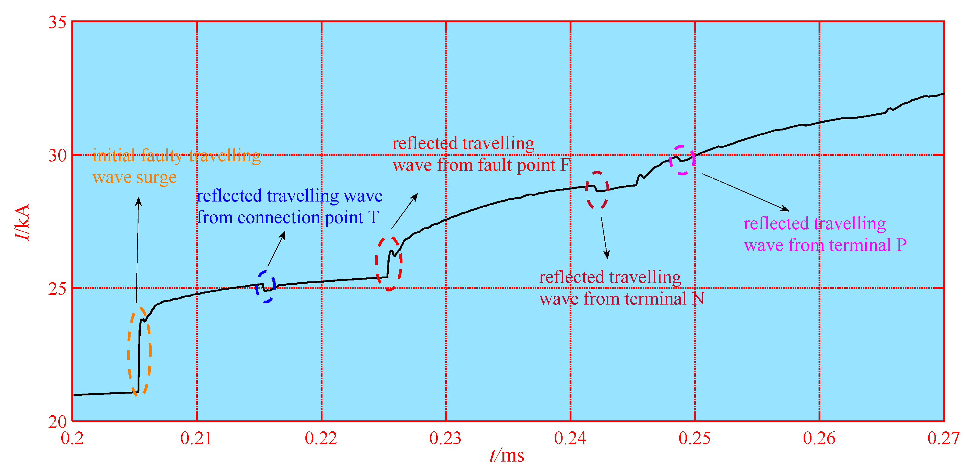
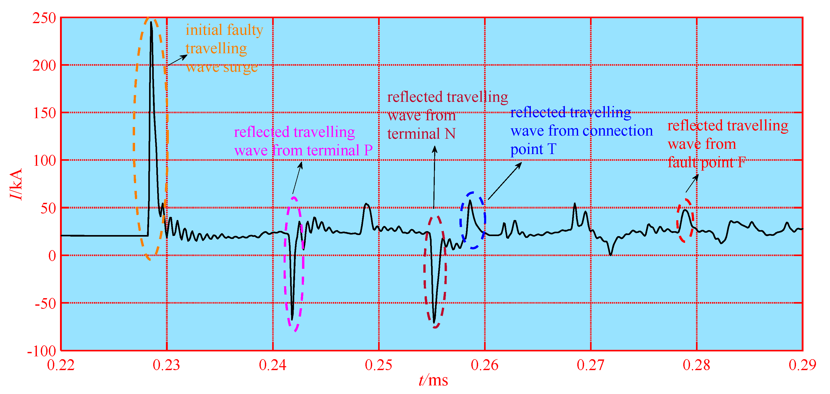
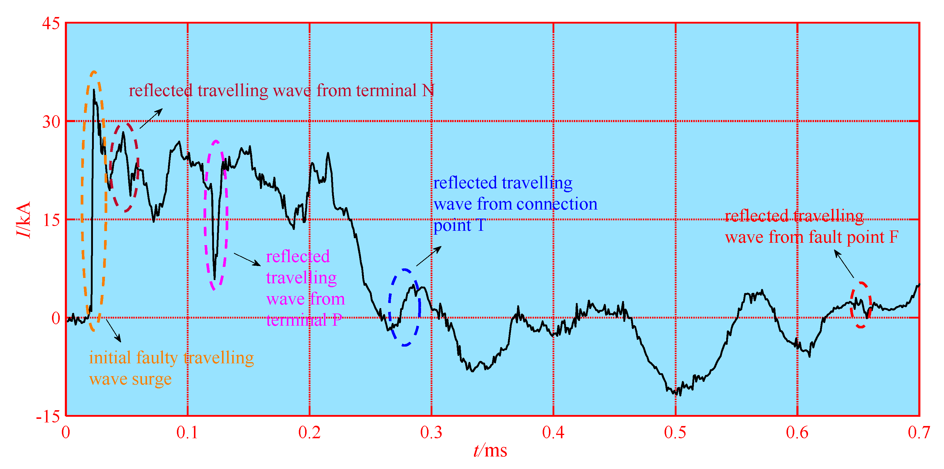
It is supposed in this paper that t₀, t_F, t_T, t_N, t_P are the times of the travelling waves arriving terminal M, which are initial travelling wave, reflected wave surge from fault point F, reflected travelling wave from connection point T, reflected travelling wave from terminal N and reflected travelling wave from terminal P. The time of travelling wave surges arriving terminal M are listed in

Table 1. Travelling wave types with their reach times.

Time	Travelling Wave Surge Types
t0	Initial travelling wave
tF	Reflected travelling wave from F
tT	Reflected travelling wave from T
tN	Reflected travelling wave from N
tP	Reflected travelling wave from P

.

Under this assumption, it is necessary to analyze the possible quantitative relationship between $x_{\mathrm{F}}$, $l_1-x_{\mathrm{F}}$, and $l_1+l_2-x_{\mathrm{F}}$. There are three situations among $x_{\mathrm{F}}$, $l_1-x_{\mathrm{F}}$, and $l_1+l_2-x_{\mathrm{F}}$, which is $x_{\mathrm{F}}<l_1-x_{\mathrm{F}}<l_1+l_2-x_{\mathrm{F}}$, $l_1-x_{\mathrm{F}}<x_{\mathrm{F}}<l_1+l_2-x_{\mathrm{F}}$, and $l_1-x_{\mathrm{F}}<l_1+l_2-x_{\mathrm{F}}<x_{\mathrm{F}}$.

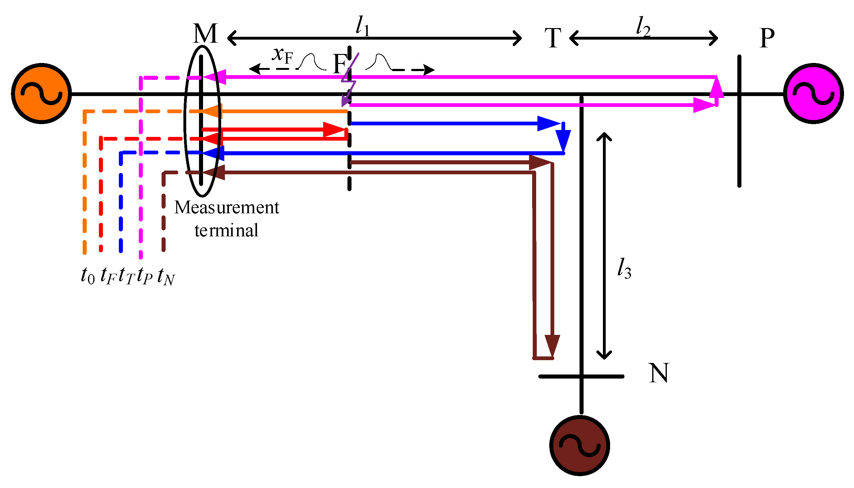
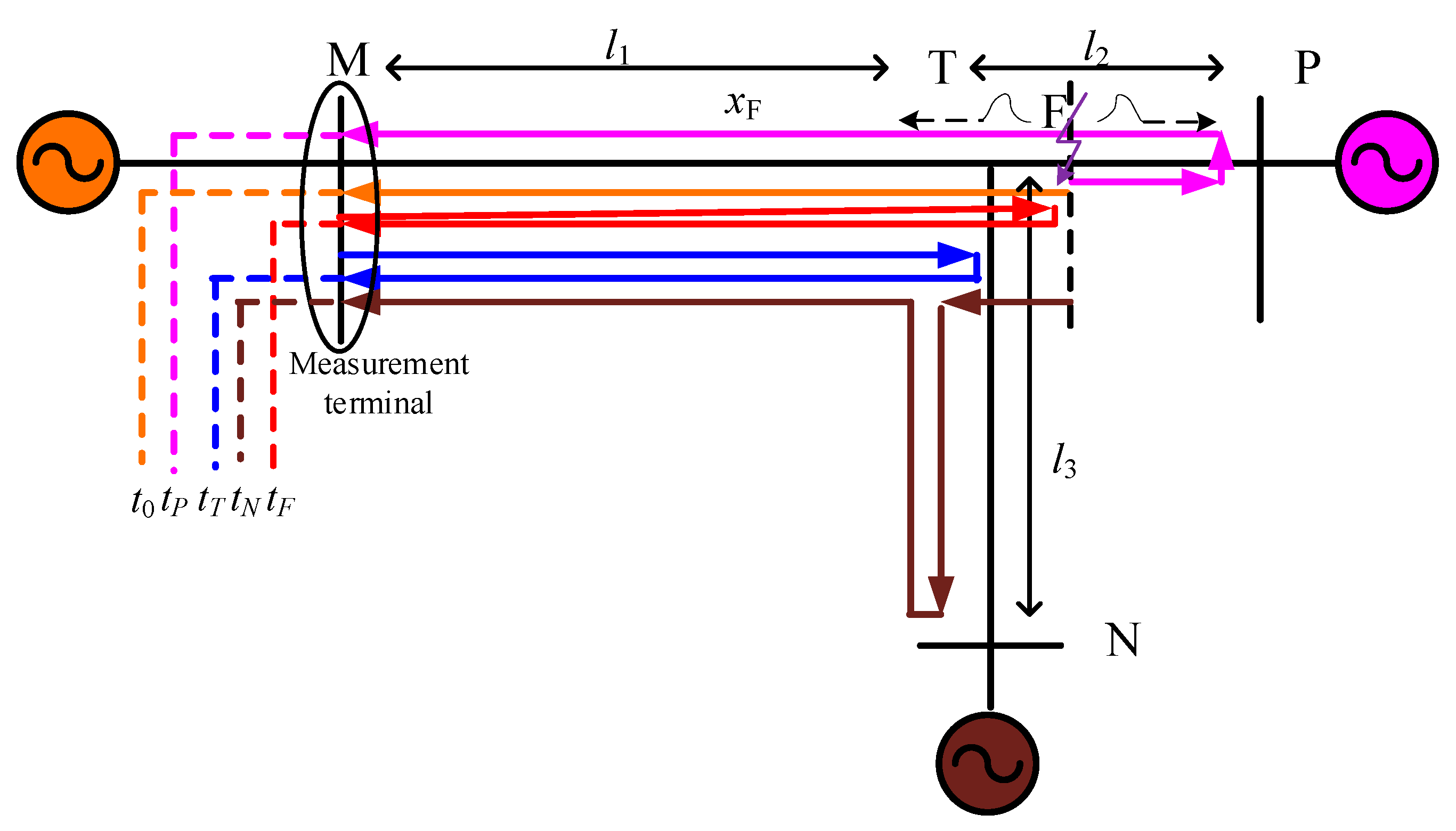
(1) If the fault occurs in the range from M to T and the fault distance satisfies $x_{\mathrm{F}}<l_1-x_{\mathrm{F}}<l_1+l_2-x_{\mathrm{F}}$, the travelling wave propagation path of the T-connection transmission line is shown in Figure 2.

The time and the propagation paths of travelling waves arriving the terminal M are listed in

Table 2. Travelling wave types with their reach times.

Time	Travelling Wave Types	Propagation Paths
t0	initial fault travelling wave	F→M
tF	reflected travelling wave from F	F→M→F→M
tT	reflected travelling wave from T	F→T→F→M
tP	reflected travelling wave from P	F→T→P→T→F→M
tN	reflected travelling wave from N	F→T→N→T→F→M

.

The distance between the initial travelling wave and the reflected travelling wave from the fault point F is $2x_{\mathrm{F}}$. The relationship of t₀, t_F, t_T, t_P and t_N can be determined as follows:

$$\{\begin{array}{l}{t}_F=t_0+2x_{\mathrm{F}}/v\\ t_T=t_0+2(l_1-x_{\mathrm{F}})/v\\ t_P=t_0+2(l_1+l_2-x_{\mathrm{F}})/v\\ t_N=t_0+2(l_1+l_3-x_{\mathrm{F}})/v\end{array}$$

(1)

In this case, $x_{\mathrm{F}}<l_1-x_{\mathrm{F}}<l_1+l_2-x_{\mathrm{F}}$, it is not difficult to see that $t_T-t_F=2(l_1-2x_{\mathrm{F}})/v>0$. Therefore, the reflected travelling wave from the fault point F reaches the measuring terminal M earlier than the reflected travelling wave from the connection point T. Thus, it can be clearly seen from Figure 2 that t₀<t_F<t_T<t_P<t_N.

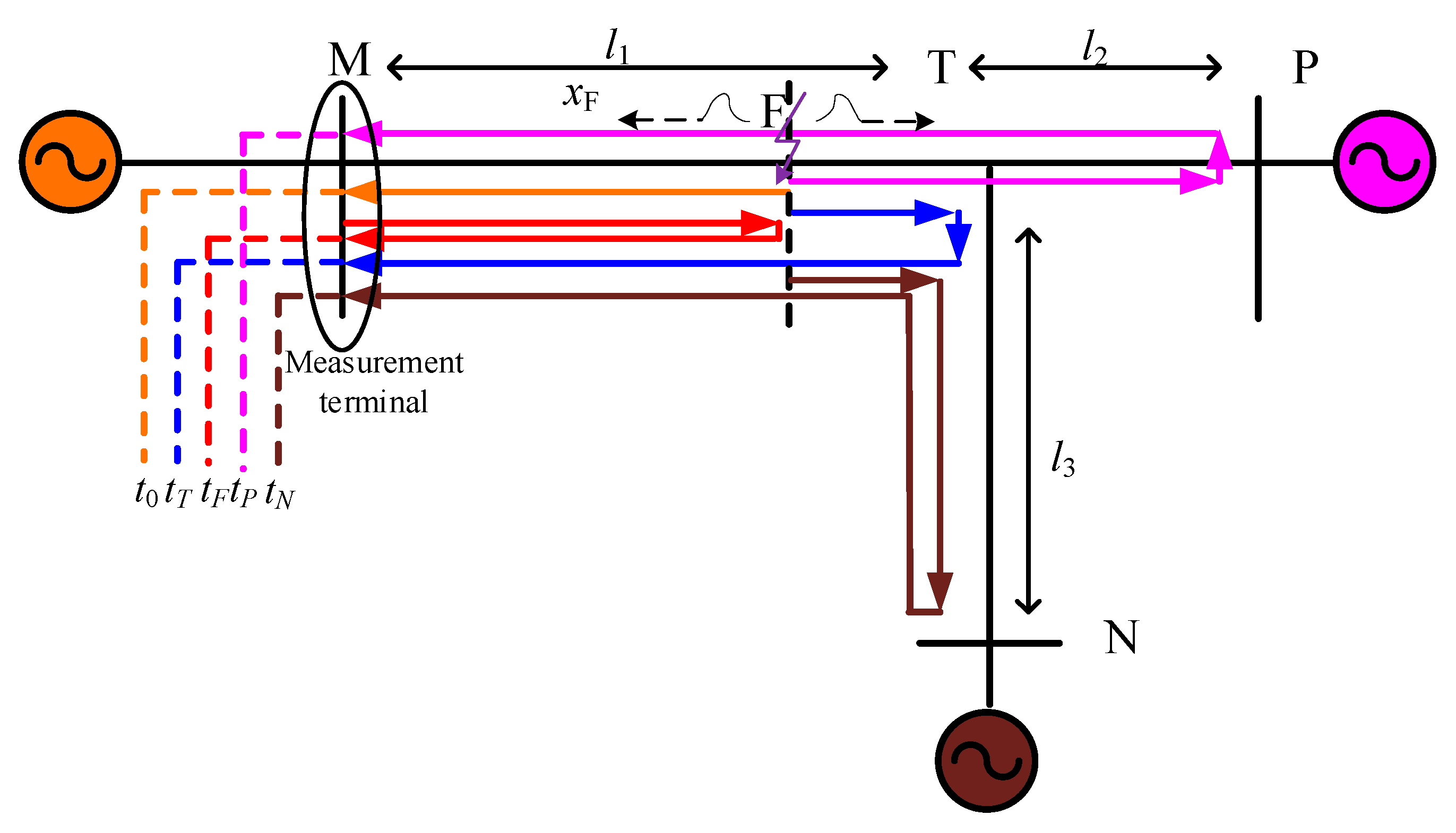
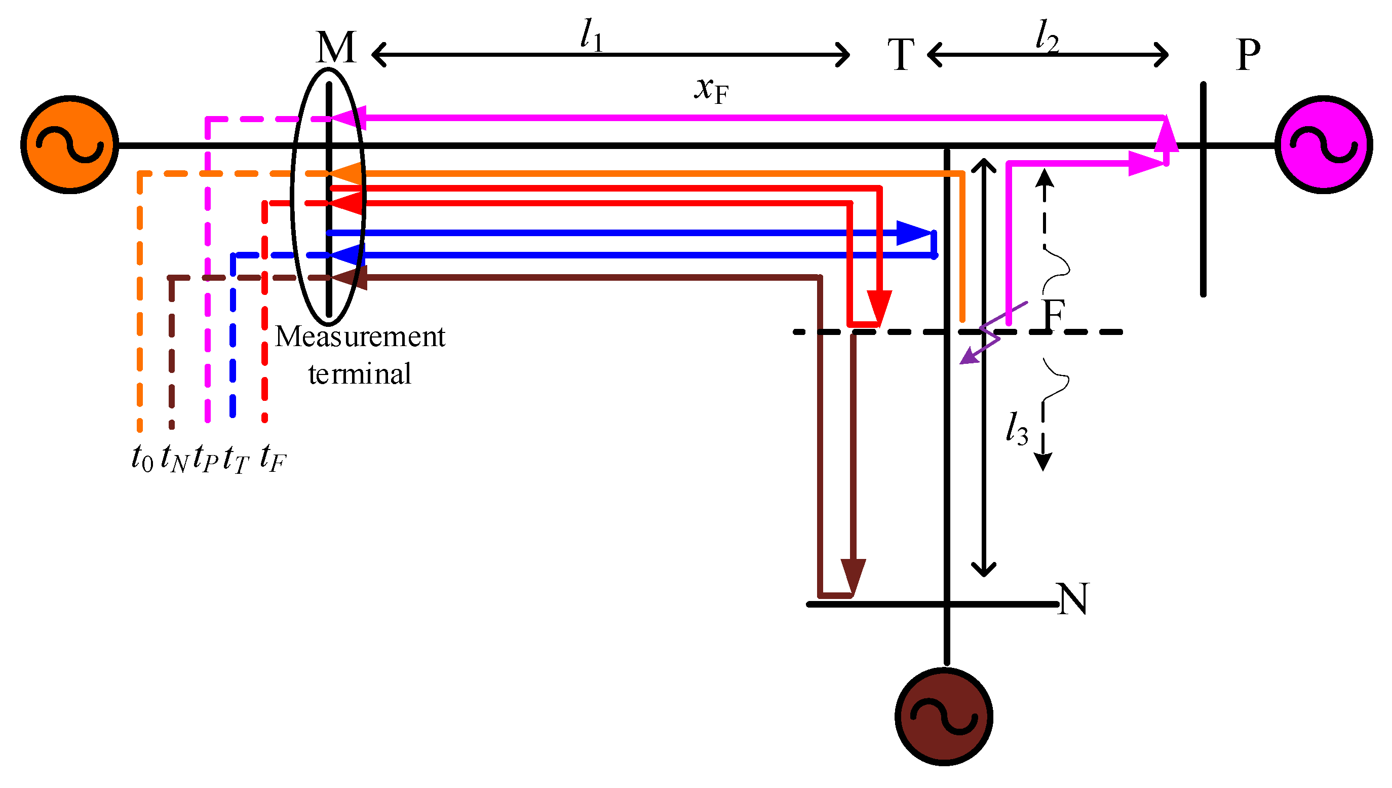
(2) If the fault occurs in the range from the terminal M to the connection point T with relationship of $l_1-x_{\mathrm{F}}<x_{\mathrm{F}}<l_1+l_2-x_{\mathrm{F}}$, the travelling wave propagation path of the T-connection transmission line is shown in Figure 3.

The time of travelling waves arriving the terminal M and the propagation paths are listed in

Table 3. Travelling wave types with their reach times.

Time	Travelling Wave Types	Propagation Paths
t0	initial fault travelling wave	F→M
tT	reflected travelling wave from T	F→T→F→M
tF	reflected travelling wave from F	F→M→F→M
tP	reflected travelling wave from P	F→T→P→T→F→M
tN	reflected travelling wave from N	F→T→N→T→F→M

.

The distance between the initial travelling wave and the reflected travelling wave from connection point T is $2(l_1-x_{\mathrm{F}})$. The relationship of t₀, t_T, t_F, t_P and t_N can be determined as follows:

$$\{\begin{array}{l}{t}_T=t_0+2(l_1-x_{\mathrm{F}})/v\\ t_F=t_0+2x_{\mathrm{F}}/v\\ t_P=t_0+2(l_1+l_2-x_{\mathrm{F}})/v\\ t_N=t_0+2(l_1+l_3-x_{\mathrm{F}})/v\end{array}$$

(2)

In this situation, $l_1-x_{\mathrm{F}}<x_{\mathrm{F}}<l_1+l_2-x_{\mathrm{F}}$, which causes $t_F-t_T=2(2x_{\mathrm{F}}-l_1)/v>0$, hence, it can be concluded that the reflected travelling wave from the connection point T reaches the measuring terminal M earlier than the reflected travelling wave from the fault point F. From Equation (2), it is easy to determine t₀<t_T<t_F<t_P<t_N.

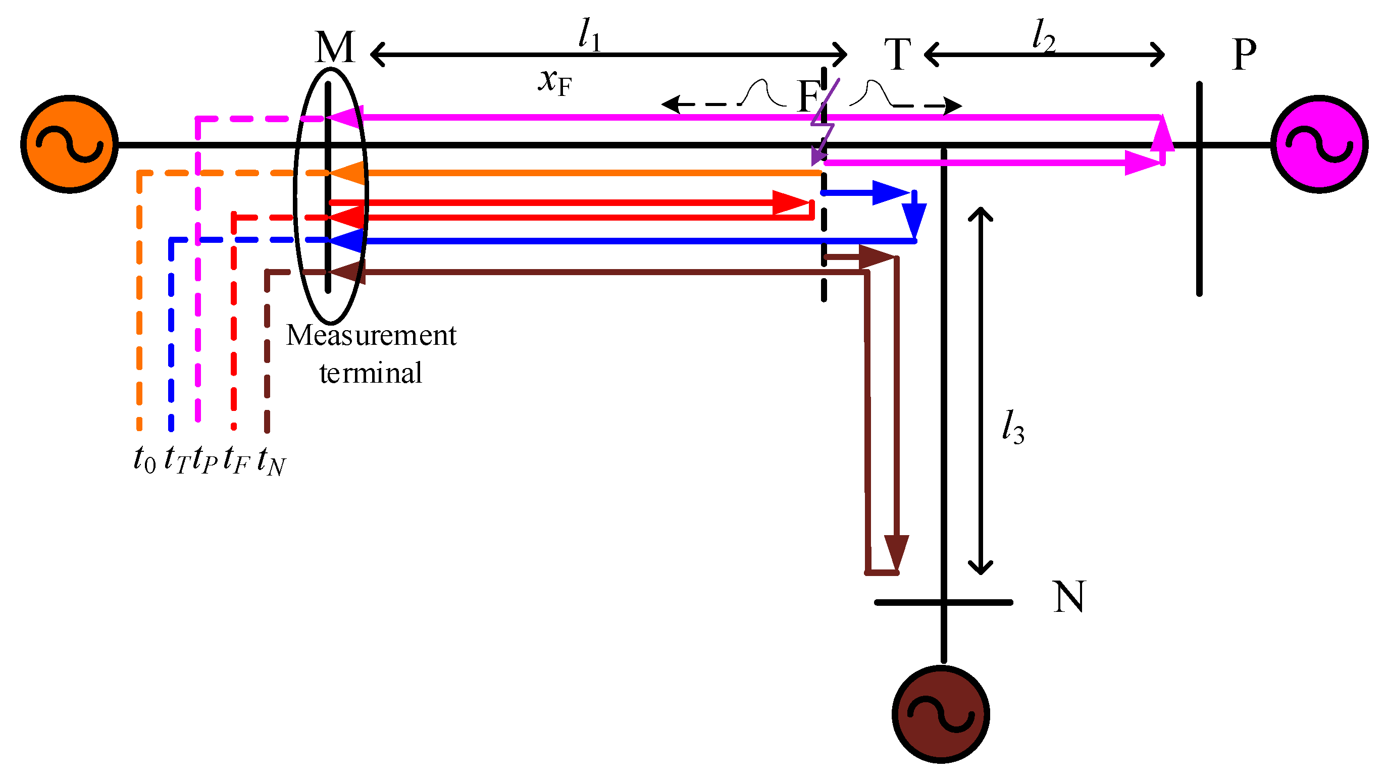
(3) If the fault occurs in the range from terminal M to connection point T within the relationship of $l_1-x_{\mathrm{F}}<l_1+l_2-x_{\mathrm{F}}<x_{\mathrm{F}}$, the travelling wave propagation path of the T-connection transmission line is shown in Figure 4.

The times of travelling waves arriving terminal M are listed in

Table 4. Travelling wave types with their reach times.

Time	Travelling Wave Types	Propagation Paths
t0	initial fault travelling wave	F→M
tT	reflected travelling wave from T	F→T→F→M
tP	reflected travelling wave from P	F→T→P→T→F→M
tF	reflected travelling wave from F	F→M→F→M
tN	reflected travelling wave from N	F→T→N→T→F→M

.

The distance between the initial travelling wave and the reflected travelling wave from connection point T is $2(l_1-x_{\mathrm{F}})$. The relationship of t₀, t_T, t_P, t_F and t_N can be determined as follows:

$$\{\begin{array}{l}{t}_T=t_0+2(l_1-x_{\mathrm{F}})/v\\ t_P=t_0+2(l_1+l_2-x_{\mathrm{F}})/v\\ t_F=t_0+2x_{\mathrm{F}}/v\\ t_N=t_0+2(l_1+l_3-x_{\mathrm{F}})/v\end{array}$$

(3)

Under this assumption, $l_1-x_{\mathrm{F}}<l_1+l_2-x_{\mathrm{F}}<x_{\mathrm{F}}$, $t_F-t_T=2(2x_{\mathrm{F}}-l_1)/v>0$, the reflected travelling wave from the connection point T reaches the measuring terminal M earlier than the reflected travelling wave from the fault point F. From Equation (3), it is easy to determine t₀<t_T<t_P<t_F<t_N.

2.2. Travelling Wave Propagation Characteristics of Faults in Section TP

When the fault occurs at the section TP, the fault travelling wave propagation path is shown in Figure 5.

The times of travelling waves arriving terminal M are listed in

Table 5. Travelling wave types with their reach times.

Time	Travelling Wave Types	Propagation Paths
t0	initial fault travelling wave	F→M
tP	reflected travelling wave from P	F→P→F→T→M
tN	reflected travelling wave from N	F→T→N→T→M
tT	reflected travelling wave from T	F→T→M→T→M
tF	reflected travelling wave from F	F→T→M→T→F→T→M

.

In the condition shown in Figure 5, the distance between the initial travelling wave and the reflected travelling wave from terminal P is $2(l_1+l_2-x_{\mathrm{F}})$. The relationship of t₀, t_P, t_T, t_N and t_F can be determined as follows:

$$\{\begin{array}{l}{t}_P=t_0+2(l_1+l_2-x_{\mathrm{F}})/v\\ t_N=t_0+2l_3/v\\ t_T=t_0+2l_1/v\\ t_F=t_0+2x_{\mathrm{F}}/v\end{array}$$

(4)

Under this condition, it is not difficult to see that $t_N-t_P=2(l_3+x_{\mathrm{F}}-l_1-l_2)/v>0$, therefore, it can be concluded that the reflected travelling wave from the terminal P reaches the measuring terminal M earlier than the reflected travelling wave from the terminal N. Besides $t_T-t_N=2(l_1-l_3)/v>0$, $t_F-t_T=2(x_{\mathrm{F}}-l_1)/v>0$, it is easy to determine t₀<t_P<t_N<t_T<t_F.

2.3. Travelling Wave Propagation Characteristics of Faults in Section TN

When the fault occurs at the section of TN, the situation is more complex than mentioned above. The fault travelling wave propagation path is shown in Figure 6.

The distance between the initial travelling wave and the reflected travelling wave from terminal N is $2(l_1+l_3-x_{\mathrm{F}})$. The relationship of t₀, t_N, t_P, t_T, and t_F can be determined as follows:

$$\{\begin{array}{l}{t}_N=t_0+2(l_1+l_3-x_{\mathrm{F}})/v\\ t_P=t_0+2l_2/v\\ t_T=t_0+2l_1/v\\ t_F=t_0+2x_{\mathrm{F}}/v\end{array}$$

(5)

In this condition, we cannot determine which of the reflected travelling waves from terminal P and the reflected travelling wave from terminal N reaches the terminal M first, because the relationship between $t_P-t_N=2(l_2+x_{\mathrm{F}}-l_1-l_3)$ and 0 cannot be judged. However, this does not affect the judgment of the fault section, because only when the section TN is faulty, the two travelling waves that finally arrived at terminal M are the reflected travelling wave from the connection point T and the reflected travelling wave from fault point F. Moreover, no matter whether the reflected travelling wave from terminal N reaches the terminal M first or the reflected travelling wave from terminal P first reaches the terminal M, their time relationship with the arrival time of the initial wave will not change, as shown in Equation (5). The times of travelling waves arriving terminal M are listed in

Table 6. Travelling wave types with their reach times.

Time	Travelling Wave Types	Propagation Paths
t0	initial fault travelling wave	F→M
tN	reflected travelling wave from N	F→N→F→T→M
tP	reflected travelling wave from P	F→T→P→T→M
tT	reflected travelling wave from T	F→T→M→T→M
tF	reflected travelling wave from F	F→T→M→T→F→T→M

. In this table, the positional relationship of t_N and t_P may be reversed. Therefore, it is easy to determine t₀<t_P<t_N<t_T<t_F, or t₀<t_N<t_P<t_T<t_F.

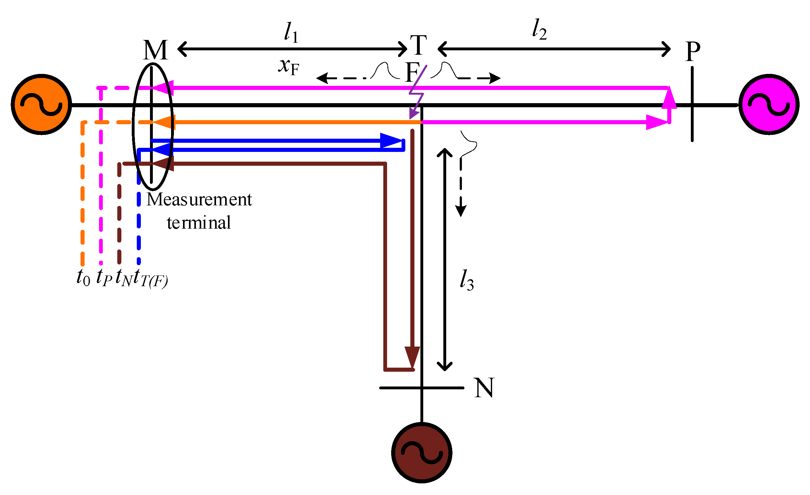
2.4. Analysis of Connection Point T Fault Travelling Wave Propagation Characteristics

If the fault occurs at the connection point T, this case is the most special of all cases. The reflected travelling wave from the fault point T and the reflected travelling wave from the connection point T is coincided. The fault travelling wave propagation path is shown in Figure 7.

In this case, it is only necessary to establish the relationship between the initial travelling wave and the reflected travelling wave from the connection point T, the reflected travelling wave from the terminal P, and the reflected travelling wave from terminal N. The distance between the initial travelling wave and the reflected travelling wave from terminal P is $2l_2$. The distance between the initial travelling wave and the reflected travelling wave from terminal N is $2l_3$. The distance between the initial travelling wave and the reflected travelling wave from the connection point T (the reflected travelling wave from fault point F) is $2x_{\mathrm{F}}$. The relationship of t₀, t_P, t_N, t_T(t_F) can be determined as follows:

$$\{\begin{array}{l}{t}_P=t_0+2l_2/v\\ t_N=t_0+2l_3/v\\ t_T(t_F)=t_0+2x_{\mathrm{F}}/v\end{array}$$

(6)

The times of travelling waves arriving terminal M are listed in

Table 7. Travelling wave types with their reach times.

Time	Travelling Wave Types	Propagation Paths
t0	initial fault travelling wave	F(T)→M
tP	reflected travelling wave from P	F(T)→P→F(T)→M
tN	reflected travelling wave from N	F(T)→N→F(T)→M
tT(tF)	reflected travelling wave from Treflected travelling wave from F	T(F)→M→T(F)→MF(T)→M→F(T)→M

.

In this case, it is not difficult to see that $t_N-t_P=2(l_3-l_2)/v>0$, therefore, it can be concluded that the reflected travelling wave from the terminal P reaches the measuring terminal M earlier than the reflected travelling wave from the terminal N. Besides $t_T(t_F)-t_N=2(x_F-l_3)/v>0$, it is easy to determine t₀ < t_P < t_N < t_T(t_F).

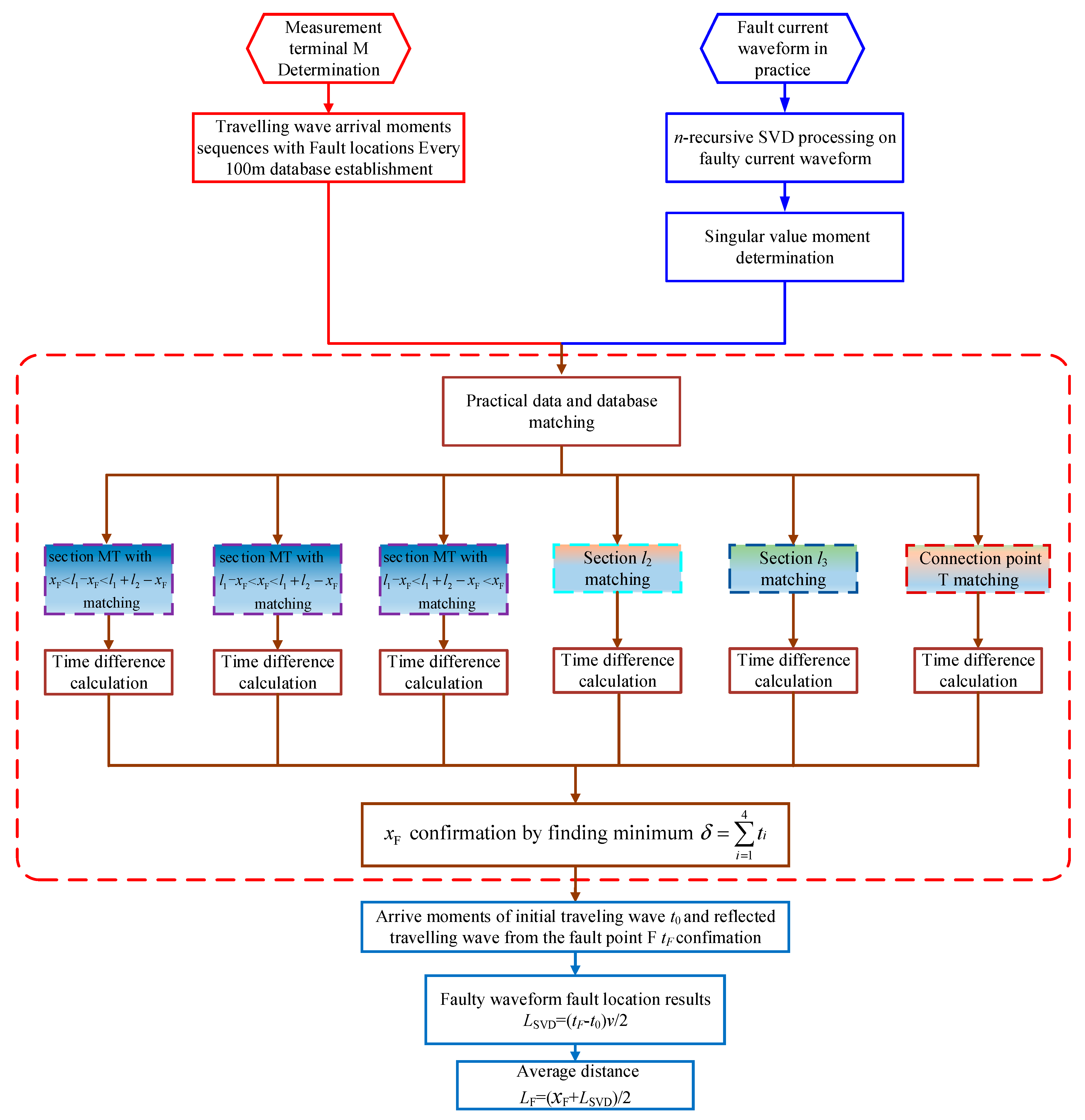
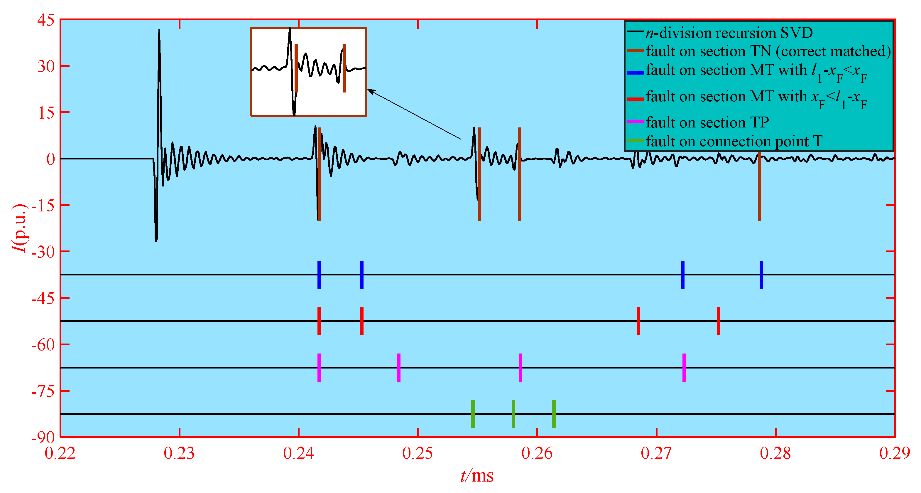
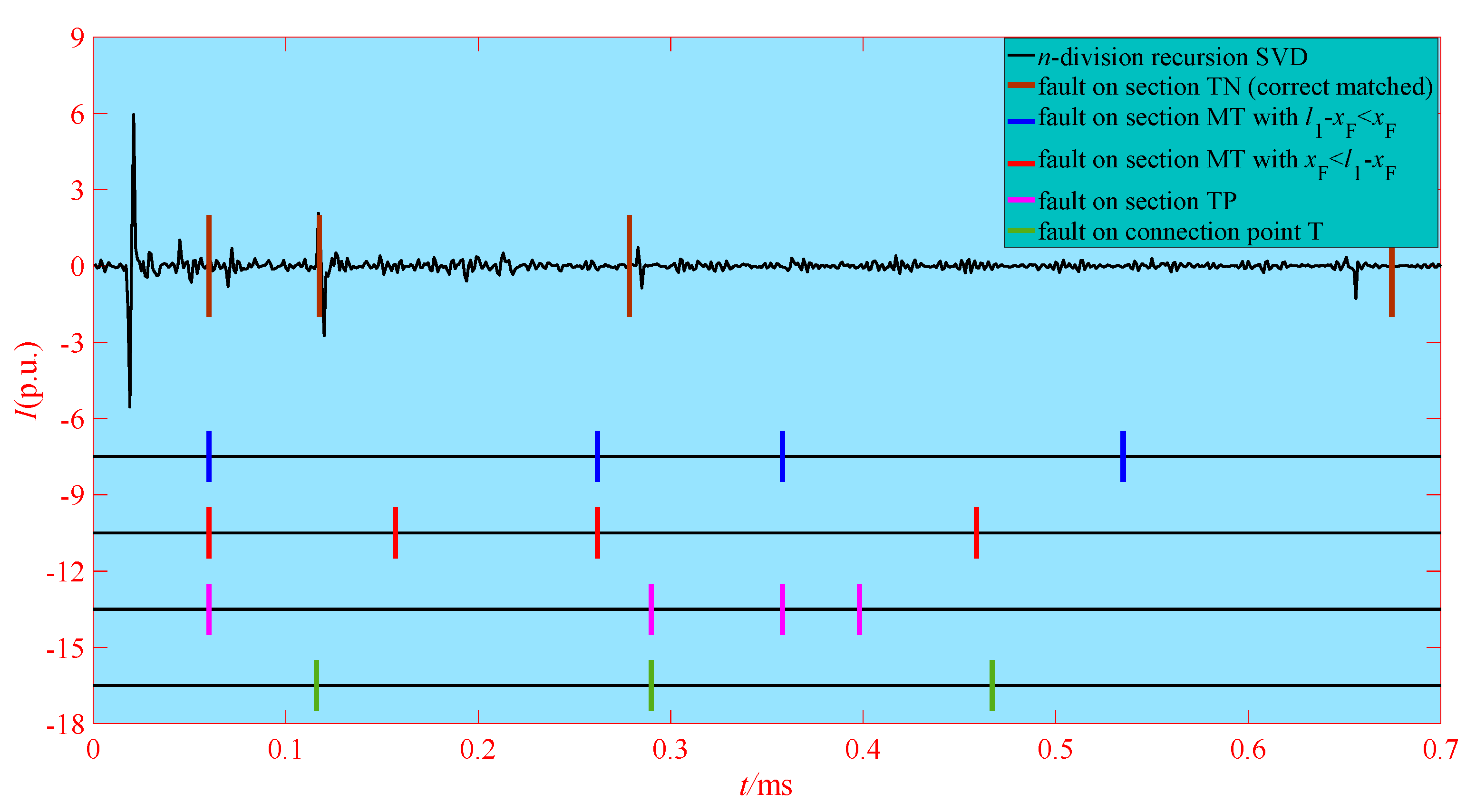
By analyzing the above fault conditions, it can be found that when the fault occurs on any point of the T-connection transmission line, there is a specific travelling wave sequence, which corresponds to the location of the fault point. In other words, a specific travelling wave sequence corresponds to only one fault point on the T-connection transmission line. In order to identify the faulty section and locate the fault point, a collection of the sequences of travelling wave arriving time is established. In this collection, each data is simulated as a fault point in the transmission line with different fault location to obtain the arrival moment of reflected travelling wave from fault point F, reflected travelling wave from connection point T, reflected travelling wave from terminal N, and reflected travelling wave from terminal P. Finally, the sequence of the travelling waves of the researched data is applied to compare with the data in the collection.

3. Signal Singularity Detection Method of Multiple Recursive SVD

SVD is a method of numerical analysis with clear physical significance, so it has been applied in many fields [31,32,33]. SVD can represent a relatively complex matrix with a relatively simple matrix. These simple matrices describe the important characteristics of the matrix.

3.1. Principle of Singular Value Decomposition

SVD is the decomposition of a matrix H of length m × n into an orthogonal matrix $U=(u_1,u_2,\dots ,u_n)\in R^{m\times m}$ and an orthogonal matrix $V=(v_1,v_2,\dots ,v_n)\in R^{n\times n}$. For the generally complex valued elements’ matrix H, SVD is obtained by factorizing it into a product of three matrices as follows in Equation (7):

$$H=US{V}^T$$

(7)

where S is an m × n matrix whose elements are zero except possibly along the main diagonal (the singular values of H), $\mathrm{S}=\left[\mathrm{diag}\right({\sigma }_1,{\sigma }_2,\cdot \cdot \cdot ,{\sigma }_{\mathrm{n}}\left)\right]$ or it is transposed, depending on whether m≤n or m>n, $S\in R^{m\times n}$, $q=\min (m,n)$, while ${\sigma }_1\ge {\sigma }_2\ge \cdots \ge {\sigma }_q>0$, ${\sigma }_{\mathrm{i}}(i=1,2,\cdots ,q)$ are the singular values of matrix H [34].

3.2. n-Division Recursive SVD Algorithm

Although the dichotomous recursive SVD method has a good detection effect on singular points, but it has a poor effect on signal noise reduction. Based on this feature, this paper improves the dichotomous recursion method and proposes an n-division recursion SVD method that can effectively suppress noise. The principle of the n-recursive SVD method is as follows:

A discrete signal $X=(x_1,x_2,\dots ,x_N)$ is sent, N is the original signal length, and an $n\times (N+1-n)$-dimensional Hankel matrix H is constructed for the original signal, $H\in R^{(N+1-n)\times n}$:

$$H=\left(\begin{array}{cccc}{x}_1& x_2& \cdots & x_n\\ x_2& x_3& \cdots & x_{n+1}\\ ⋮& ⋮& \cdots & ⋮\\ x_{N+1-n}& x_{N+2-n}& \cdots & x_N\end{array}\right)$$

(8)

By performing SVD on the H matrix, n singular values can be obtained. In the matrix H, starting from the second row, each row lags one data later than the previous row, and the correlation between the two rows of data is high. H can be rewritten as a vector u_i and v_i according to Equation (9):

$$H={\sigma }_{i1}{u}_{\mathrm{i}1}{v_{i1}}^T+{\sigma }_{i2}{u}_{i2}{v_{i2}}^T+\cdots +{\sigma }_{in}{u}_{in}{v_{in}}^T$$

(9)

in Equation (9), $u_i\in R^{n\times (N+1-n)}$, $v_i\in R^{(N+1-n)\times (N+1-n)}$, i=1,2……, n. We command $H_1={\sigma }_{i1}{u}_{i1}{v_{i1}}^T$, so $H_1\in R^{n\times \left(N+1-n\right)}$. The structure of H₁ is similar to H, but not identical, H₁ is just a detail matrix that can best reflect the H information of the original signal, and the specific expression of H₁ shown in Equation (10):

$$H_1=\left(\begin{array}{cccc}{H}_1(1,1)& H_1(1,2)& \cdots & H_1(1,N+1-n)\\ H_1(2,1)& H_1(2,2)& \cdots & H_1(2,N+2-n)\\ ⋮& ⋮& \cdots & ⋮\\ H_1(n,1)& H_1(n+1,1)& \cdots & H_1(n,N)\end{array}\right)$$

(10)

In the matrix H₁, H₁(n,1)=H₁(n-1,2)=…= H₁(1, n) should be satisfied. In the same way, $H_2={\sigma }_{i2}{u}_{i2}{v_{i2}}^T$ to $H_{\mathrm{n}}={\sigma }_{in}{u}_{in}{v_{in}}^T$ can be calculated as above [35].

Each layer of the n-division recursion SVD is a further fine characterization of the original signal, but at the same time the energy of the detailed component signal of each layer also decreases accordingly. It is particularly important to be able to adaptively determine an optimal decomposition layer according to the target signal. Referring to the concept of information entropy, a singular entropy is introduced to represent the uncertainty of the variable. The calculation method as shown in Equation (11):

$$E=-{\displaystyle \sum _{i=1}^m\left[\left({\sigma }_i/{\displaystyle \sum _{k=1}^m{\sigma }_k}\right)\log \left({\sigma }_i/{\displaystyle \sum _{k=1}^m{\sigma }_k}\right)\right]}$$

(11)

In Equation (11), m is the number of singular values, and ${\sigma }_i/{\displaystyle \sum _{k=1}^m{\sigma }_k}$ is the weight of the i-th singular value to all singular values. The singular entropy reflects the uncertainty of the signal singularity energy distribution. The fuzzier the signal singularity is, the more concentrated the energy distribution is on a few singular values, and the smaller the signal singular entropy; on the contrary, the more obvious the signal singularity, the more dispersed the energy, and the larger the signal singular entropy. After the n-level multi-scale SVD, n detail component matrices and one approximate component matrix can be obtained. The new matrix composed of n + 1 matrices can represent all the information of the original signal. According to the SVD theory, the singular value of a matrix can reflect the entire amount of information of the matrix. When the number of decomposition layers is increased to a certain extent, if the singular entropy of the new matrix does not increase significantly, the number of decomposition layers is considered to be optimal.

We define the n-th layer singular entropy increment ΔE_n as:

$$\mathsf{\Delta }{E}_n=\frac{E_n-E_{n-1}}{E_{n-1}}$$

(12)

where n≥2. If ΔE obviously approaches to 0, it is not necessary to continue the decomposition, and the number of decomposition layers reaches the optimal. By decomposing the travelling wave data with different layers, the singular entropy results are tabulated in

Table 8. Singular entropy increments with different decomposition layers.

n	ΔE(p.u.)
2	0.082
3	0.0081
4	0.0048
5	0.0012

. It can be concluded from Table 8 that the singular entropy decreases with the increase of the decomposition layer. However, the decreasing of the singular entropy is much slower if the decomposition layer is larger than 3. Therefore, the decomposition is chosen as 3.

3.3. Single-Terminal Fault Location Scheme for T-Connection Transmission Line

The selection of the fault time window plays a vital role in the realization of travelling wave fault location. When the time window is too short, the travelling wave required for fault location may not be within the selected time window. Loss of important information required for fault location will directly lead to failure. If the time window selected is too long, the reflection waves of various nodes that are not needed for fault location and more noise interference will appear in the time window. The extra travelling wave may lead to incorrect results in fault location. In this method, full consideration should be given to the time window containing the fault point reflected travelling wave, reflected travelling wave from the connection point, reflected travelling wave from the terminal N and reflected travelling wave from the terminal P. The length of the time window determined by Equation (13):

$${\mathrm{T}}_{\mathrm{W}}=\max \left[2\right(l_1+l_2)/v,2(l_1+l_3)/v]$$

(13)

In Equation (13), max represents the maximum value, l₁, l₂, and l₃ represent the distances from the connection point T to the three terminals, the bus at the terminal M is the measurement terminal, and v is the travelling wave velocity.

A fault point $x_{\mathrm{F}}$ is set every 100 m from the terminal M to calculate the time of different reflected travelling wave arriving the terminal M. Then, all the calculated sequences are applied to form a collection as the fault cases. After extracting the sequence of travelling waves by SVD, the specific fault data are compared with the sequences of travelling waves in the collection. Owing to the uniqueness of the travelling wave arrival sequence, the faulty section and the fault point can be determined by the comparison of cases in the collection. In order to measure the differences of the sequence of the specific data and the data in the collection, δ is calculated by the sum of time differences.

$$\delta ={\displaystyle \sum _{i=1}^{4}ti}$$

(14)

In Equation (14), t_i represents the time difference between the travelling wave moments calculation and the original fault signal after n-division recursive SVD, and i represents the different travelling waves that reach the measurement terminal M, as shown in

Table 9. Meanings of t_i.

ti	Time Difference
1	Time difference of reflected travelling waves from F of the specific data and the data in the collection
2	Time difference of reflected travelling waves from T of the specific data and the data in the collection
3	Time difference of reflected travelling waves from P of the specific data and the data in the collection
4	Time difference of reflected travelling waves from N of the specific data and the data in the collection

.

δ, which represents the similarity of the sequences, decreases with the increasing of the similarity of two sequences.

When the matching algorithm is satisfied, the matched fault distance $x_{\mathrm{F}}$ is determined, while t₀, t_F are determined by $x_{\mathrm{F}}$. The fault distance of the reflected travelling wave corresponding to the fault point F of the n-recursion SVD method calculated as shown in Equation (15):

$$L_{\mathrm{SVD}}=(t_F-t_0)v/2$$

(15)

In Equation (15) presents the fault distance calculated by the n-recursive SVD calibration wave; t₀ is the arrival time of the travelling wave from the fault point, and t_F is the arrival moment of the reflected travelling wave from the fault point F. Finally, by averaging the distance calculated by the full-line matching algorithm and the fault distance calculated by the n-recursive recursion method, the final fault location result is obtained. We used the hypothesis result $x_{\mathrm{F}}$ and the waveform calculation result L_n to obtain the average value, which can make the fault point location result more accurate. The algorithm flowchart is shown in Figure 8.

4. Case Study

4.1. Simulation Model

PSCAD/EMTDC of version 4.5 [36,37,38,39] with sampling rate of 1 MHz is implemented to simulate the faults in the T-connection transmission lines as demonstrated in Figure 1, and its parameters are given in

Table 10. Parameters of transmission lines.

Mode	Resistance (Ω/km)	Inductance (H/km)	Capacitance (F/km)
positive sequence	1.1598 × 10−1	1.3134 × 10−3	8.8849 × 10−9
zero sequence	4.6399 × 10−1	4.0589 × 10−3	5.9644 × 10−9

. The lengths of the T-connection transmission line are set to l₁ = 50 km, l₂ = 40 km, and l₃ = 45 km.

4.2. Single-Phase Ground Fault Simulation

A phase-to-ground (AG) fault occurs at section l₁ with fault distance $x_{\mathrm{F}}$=30 km and 20 Ω fault resistance at 0.202 s, this simulation corresponds to the $l_1-x_{\mathrm{F}}<x_{\mathrm{F}}<l_1+l_2-x_{\mathrm{F}}$ case in Section 2.1. The simulation current waveform and the result of SVD are illustrated in Figure 9.

It can be seen in the Figure 9 that the proposed method accurately detects and calibrates singular points in the transient waveform. Assume the first reflected travelling wave is from each feasible impedance discontinuity, the sequences of the travelling wave of the assumptions are compared with the result of SVD as shown in Figure 10. It can be seen that only the correct matched aligned all singular value points.

The matching result is that the fault occurred in l₁ section, and the fault distance is $x_{\mathrm{F}}$ = 30.2 km, which is quite similar to the actual fault position.

The travelling wave arrive sequence shown in Figure 11, it can calculate the fault location within the initial fault travelling wave and the reflected travelling wave from fault point F, the fault distance L_SVD = 30.1 km, so the final result is 30.15 km.

4.3. Lightning Fault Simulation

A lightning induced Phase A ground fault (AG) occurs 75 km away from the terminal M at 0.204 ms. This simulation corresponds to the $l_1-x_{\mathrm{F}}<x_{\mathrm{F}}<l_1+l_2-x_{\mathrm{F}}$ case in Section 2.3. The lightning current model adopts the double exponential model [40,41,42]. The fault phase current measured at the measuring terminal of the T-connection transmission line shown in Figure 12a. The fault phase data in Figure 12a subjected to n-division recursive SVD singularity calibration, and the result shown in Figure 12b.

The results of the combination of the full-line matching algorithm and SVD shown in Figure 13. The result of the calculation is that the fault occurred within l₃ of the fault section, and the fault distance is $x_{\mathrm{F}}$ = 75.1 km.

The travelling wave sequence shown in Figure 14 can calculate the fault location within the initial fault travelling wave and the reflected travelling wave from fault point F. The fault distance L_SVD is 75 km, so the final result is 75.05 km.

In order to fully verify the reliability of the algorithm, different types of faults (single-phase ground fault, phase-to-phase short-circuit fault, three-phase short-circuit fault, and lightning strike failure) at different fault sections (l₁, l₂, l₃, and connection point T) were simulated for the test. Owing to the page limits, a part of the simulation results is tabulated in

Table 11. Simulation results of various fault situations.

Fault Section	Fault Type	Fault Distance (km)	Calculation Results (km)	Calculation Deviation (km)
l1	Phase-to-phase short-circuit fault (AB)	15	15.16	0.16
	Three-phase short-circuit fault (ABC)	20	20.11	0.11
	Lightning strike failure (A)	35	35.08	0.08
l2	Single-phase ground fault(B)	50	50.11	0.11
	Phase-to-phase short-circuit fault (AB)	63	63.14	0.14
	Three-phase short-circuit fault (ABC)	71	71.12	0.12
	Lightning strike failure (A)	80	80.16	0.16
l3	Single-phase ground fault(B)	61	61.14	0.14
	Phase-to-phase short-circuit fault (AB)	70	70.21	0.21
	Three-phase short-circuit fault (ABC)	83	83.09	0.09
connection point T	Single-phase ground fault(B)	45	45.11	0.11
	Phase-to-phase short-circuit fault (AB)	45	45.07	0.07
	Three-phase short-circuit fault (ABC)	45	45.14	0.14
	Lightning strike failure (A)	45	45.15	0.15

.

5. Practical Field Data Test in Yunnan Province

In order to verify the accuracy of the proposed fault location method for the actual fault data, a travelling wave analysis and locating device was established, as illustrated in Figure 15. The device can complete the synchronous sampling of 16 channel records at a sampling rate of 1 MHz.

The geographical map of Yunnan Province is shown in Figure 16a, while a part of the topology of the 110 kV transmission line in Pu’er Power Grid is shown in Figure 16b. Ximahe substation, which is equipped with the established travelling wave analysis and locating device is and 38.83 km away from the connection point T, is assumed as the terminal M. Similarly, Jiangcheng substation, which is 64.83 km away from the connection point, and Laoshizhai substation, which is 14.4 km away from the connection point, are assumed as the terminal N and P, respectively. A fault induced by the transmission line swing is recorded on June 30, 2018. The measured current waveform is shown in Figure 17.

After selecting the time window of the fault phase data, the n-division recursive SVD transformation is applied to detect the wavefronts. The result of SVD is compared with all the assumptions as shown in Figure 18. The types of travelling waves are illustrated in Figure 19.

By the n-division recursive SVD for comparison, it can be correctly identified that the faulty section is the terminal P, the fault distance is 97.1 km away from the terminal M. The actual line inspection result is 97.4 km, which is only 0.3 km different from the fault location result.

6. Conclusions

This paper presents a single terminal fault location algorithm for T-connection transmission lines based on the sequences of travelling waves, which is able to accurate identify the faulty section and locate the fault point. The main contributions of this paper can be summarized into the following three aspects:

(1) This paper discusses the sequence of fault induced travelling waves reaching the measuring terminal to manifest the uniqueness of the sequences of different fault points. A reliable single-terminal fault location method for T-connection transmission lines is proposed, which does not need to identify the travelling wave property of the fault current waveform.

(2). This paper uses the n-recursive SVD to obtain accurate singular value information of the original fault current signal, and then finds the assumed fault location that best matches the fault signal by calculating the singular value information.

(3). Simulation results of different case studies and the practical field data have verified that the proposed method is able to accurately identify the faulty section and locate fault point.

References

1. Saber, A.; Emam, A.; Elghazaly, H. A backup protection technique for three-terminal multisection compound transmission lines. IEEE Trans. Smart Grid 2018, 9, 5653–5663. [Google Scholar] [CrossRef]
2. Maheshwari, Z.; Ramakumar, R. Smart integrated renewable energy systems (SIRES): A novel approach forsustainable development. Energies 2017, 10, 1145. [Google Scholar] [CrossRef]
3. Yang, B.; Zhang, X.S.; Yu, T.; Shu, H.C.; Fang, Z.H. Grouped grey wolf optimizer for maximum power point tracking of doubly-fed induction generator based wind turbine. Energy Convers. Manag. 2017, 133, 427–443. [Google Scholar]
4. Yang, B.; Wang, J.B.; Zhang, X.S.; Yu, T.; Yao, W.; Shu, H.C.; Zeng, F.; Sun, L.M. Comprehensive overview of meta-heuristic algorithm applications on pv cell parameter identification. Energy Convers. Manag. 2020, 208, 112595. [Google Scholar] [CrossRef]
5. Li, G.D.; Li, G.Y.; Zhou, M. Model and application of renewable energy accommodation capacity calculation considering utilization level of interprovincial tie-line. Prot. Control. Mod. Power Syst. 2019, 4, 1–12. [Google Scholar] [CrossRef]
6. Sun, K.; Yao, W.; Fang, J.K.; Ai, X.M.; Wen, J.Y.; Cheng, S.J. Impedance modeling and stability analysis of grid-connected DFIG-based wind farm with a VSC-HVDC. IEEE J. Emerg. Sel. Top. Power Electron. 2019. [Google Scholar] [CrossRef]
7. Yang, B.; Zhong, L.E.; Yu, T.; Li, H.F.; Zhang, X.S.; Shu, H.C.; Sang, Y.Y.; Jiang, L. Novel bio-inspired memetic salp swarm algorithm and application to MPPT for PV systems considering partial shading condition. J. Clean. Prod. 2019, 215, 1203–1222. [Google Scholar] [CrossRef]
8. Yang, B.; Jiang, L.; Wang, L.; Yao, W.; Wu, Q.H. Nonlinear maximum power point tracking control and modal analysis of DFIG based wind turbine. Int. J. Electr. Power Energy Syst. 2016, 74, 429–436. [Google Scholar] [CrossRef] [Green Version]
9. Chaibi, Y.; Allouhi, A.; Salhi1, M.; El-jouni, A. Annual performance analysis of different maximum power point tracking techniques used in photovoltaic systems. Prot. Control. Mod. Power Syst. 2019, 4, 171–180. [Google Scholar] [CrossRef]
10. Cao, P.L.; Shu, H.C.; Yang, B.; An, N.; Qiu, D.L.; Teng, W.Y.; Dong, J. Voltage Distribution–Based Fault Location for Half-Wavelength Transmission Line with Large-Scale Wind Power Integration in China. Energies 2018, 11, 593. [Google Scholar] [CrossRef] [Green Version]
11. Yao, C.G.; Wu, H.; Long, Y.; Mi, Y.; Ma, Y.; Shen, Y.; Wang, L. A novel method to locate a fault of transmission lines by shielding failure. IEEE Trans. Dielectr. Electr. Insul. 2014, 21, 1573–1583. [Google Scholar] [CrossRef]
12. Yang, B.; Yu, T.; Shu, H.C.; Zhang, Y.M.; Chen, J.; Sang, Y.Y.; Jiang, L. Passivity-based sliding-mode control design for optimal power extraction of a PMSG based variable speed wind turbine. Renew. Energy 2018, 119, 577–589. [Google Scholar] [CrossRef]
13. Zhang, Z.J.; You, J.W.; Zhao, J.Y.; Cheng, Y.; Jiang, X.L.; Li, Y.F. Contamination characteristics of disc-suspension insulator of transmission line in wind tunnel. IET Gener. Transm. Distrib. 2017, 11, 1453–1460. [Google Scholar] [CrossRef]
14. Cao, P.L.; Shu, H.C.; Yang, B.; Dong, J.; Fang, Y.; Yu, T. Speeded-up robust features based single-ended travelling wave fault location: A practical case study in Yunnan power grid of China. IET Gener. Transm. Distrib. 2018, 12, 886–894. [Google Scholar] [CrossRef]
15. Wen, F.; Yuan, L. Wide area measurements based fault detection and location method for transmission lines. Prot. Control. Mod. Power Syst. 2019, 4, 53–64. [Google Scholar]
16. Yang, B.; Yu, T.; Shu, H.C.; Jiang, L. Robust sliding-mode control of wind energy conversion systems for optimal power extraction via nonlinear perturbation observers. Appl. Energy 2018, 210, 711–723. [Google Scholar] [CrossRef]
17. Han, Y.; Xu, C.; Xu, G.; Zhang, Y.W.; Yang, Y.P. An improved flexible solar thermal energy integration process for enhancing the coal-based energy efficiency and NOx removal effectiveness in coal-fired power plants under different load conditions. Energies 2017, 10, 1485. [Google Scholar] [CrossRef] [Green Version]
18. Lin, X.; Zhao, F.; Wu, G.; Li, Z.; Weng, H. Universal WavefrontPositioning Correction Method on Travelling-Wave-Based Fault-Location Algorithms. IEEE Trans. Power Deliv. 2012, 27, 1601–1610. [Google Scholar] [CrossRef]
19. Lin, T.C.; Lin, P.Y.; Liu, C.W. An algorithm for locating faults in three-terminal multisection nonhomogeneous transmission lines using synchrophasor measurements. IEEE Trans. Smart Grid 2014, 5, 38–50. [Google Scholar] [CrossRef]
20. Swagata, D.; Sundaravaradan, N.A.; Surya, S. Estimating zero-sequence impedance of three-terminal transmission line and Thevenin impedance using relay measurement data. Prot. Control. Mod. Power Syst. 2018, 3, 373–382. [Google Scholar]
21. Liang, R.; Wang, F.; Fu, G.Q.; Xue, X.; Zhou, R. A general fault location method in complex power grid based on wide-area travelling wave data acquisition. Int. J. Electr. Power Energy Syst. 2016, 83, 213–218. [Google Scholar] [CrossRef]
22. Ray, P.; Mishra, D.P. Support vector machine based fault classification and location of a long transmission line. Eng. Sci. Technol. Int. J. 2016, 19, 1368–1380. [Google Scholar] [CrossRef] [Green Version]
23. Gilany, M.; Ibrahim, D.K.; Eldin, E. Travcling-Wave-Based Fault-Location Scheme for Multiend-Aged Underground Cable System. IEEE Trans. Power Deliv. 2007, 22, 88–89. [Google Scholar] [CrossRef]
24. Lopes, F.V.; Silba, K.M.; Casta, F.B. Real-Time Travelling-wave-Base Fault Location Using Two-terminal Unsynchronized Data. IEEE Trans. Power Deliv. 2015, 30, 1067–1069. [Google Scholar] [CrossRef]
25. Khodadadi, M.; Shahrtash, S.M. A new noncommunication-based protection scheme for three-terminal transmission lines employing mathematical morphology-based filters. IEEE Trans. Power Deliv. 2013, 28, 347–356. [Google Scholar] [CrossRef]
26. Mahamedi, B.; Sanaye-Pasand, M.; Azizi, S.; Zhu, J.G. Unsynchronized fault-location technique for three-terminal lines. IET Gener. Transm. Distrib. 2015, 9, 2099–2107. [Google Scholar] [CrossRef]
27. Mallikarjuna, B.; Shanmukesh, P.; Anmol, D.; Reddy, M.J.B.; Mohanta, D.K. PMU based adaptive zone settings of distance relays for protection of multi-terminal transmission lines. Prot. Control. Mod. Power Syst. 2018, 3, 126–140. [Google Scholar] [CrossRef] [Green Version]
28. Korkal, M.; Lev-Ari, H.; Abur, A. Travelling-wave-based fault-locationtechnique for transmission grids via wide-area synchronized voltage measurements. IEEE Trans. Power Syst. 2012, 27, 1003–1011. [Google Scholar] [CrossRef]
29. Liang, R.; Fu, G.; Zhu, X. Fault location based on single terminal travelling wave analysis in radial distribution network. Int. J. Electr. Power Energy Syst. 2015, 66, 160–165. [Google Scholar] [CrossRef]
30. Spoor, D.; Zhu, J. Improved single-ended travelling-wave fault-location algorithm based on experience with conventional substation transducers. IEEE Trans. Power Deliv. 2006, 21, 1714–1720. [Google Scholar] [CrossRef] [Green Version]
31. Phillips, R.D.; Watson, L.T.; Wynne, R.H. Feature reduction using a singular value decomposition for the iterative guided spectral class rejection hybrid classifier. ISPRS J. Photogramm. Remote Sens. 2009, 64, 107–116. [Google Scholar] [CrossRef] [Green Version]
32. Ahemd, S.M.; Alzoubi, Q.; Abozahhad, D.M. A hybrid ECG compression algorithm based on singular value decomposition and discrete wavelet transform. J. Med. Eng. Technol. 2007, 31, 54–61. [Google Scholar] [CrossRef] [PubMed]
33. Vanlanduit, S.; Cauberghe, B.; Guillaume, P. Reduction of large frequency response function data sets using robust singular value decomposition. Comput. Struct. 2006, 84, 808–822. [Google Scholar] [CrossRef]
34. Vozalis, M.G.; Margaritis, K.G. Using SVD and demographic data for the enhancement of generalized collaborative filtering. Inf. Sci. 2007, 177, 3017–3037. [Google Scholar] [CrossRef]
35. Lehtola, L.; Karsikas, M.; Koskinen, M. Effects of noise and filtering on SVD-based morphological parameters of the T wave in the ECG. J. Med. Eng. Technol. 2008, 32, 400–407. [Google Scholar] [CrossRef] [PubMed]
36. Shen, Y.; Yao, W.; Wen, J.Y.; He, H.B.; Jiang, L. Resilient wide-area damping control using GrHDP to tolerate communication failures. IEEE Trans. Smart Grid 2019, 10, 2547–2557. [Google Scholar] [CrossRef]
37. Peng, X.T.; Yao, W.; Yan, C.; Wen, J.Y.; Cheng, S.J. Two-stage variable proportion coefficient based frequency support of grid-connected DFIG-WTs. IEEE Trans. Power Syst. 2019. [Google Scholar] [CrossRef]
38. Liu, J.; Yao, W.; Wen, J.Y.; Fang, J.K.; Jiang, L.; He, H.B.; Cheng, S.J. Impact of power grid strength and PLL parameters on stability of grid-connected DFIG wind farm. IEEE Trans. Sustain. Energy 2020, 11, 545–557. [Google Scholar] [CrossRef]
39. Yang, B.; Yu, T.; Zhang, X.S.; Li, H.F.; Shu, H.C.; Sang, Y.Y.; Jiang, L. Dynamic leader based collective intelligence for maximum power point tracking of PV systems affected by partial shading condition. Energy Convers. Manag. 2019, 179, 286–303. [Google Scholar]
40. Meliopoilos, A.P.; Moharam, M.G. Transients analysis of grounding systems. IEEE Trans. Power Apparantus Syst. 1983, 102, 389–399. [Google Scholar] [CrossRef]
41. Ishii, M.; Kawamura, T. Multistory transmission tower modle for lightning analysis. IEEE Trans. Power Deliv. 1991, 6, 1327–1335. [Google Scholar] [CrossRef]
42. Whiteheda, J.T.; Chisholm, W.A.; Anderson, J.G. IEEE work group report. Estimating lightning performance of transmission lines. II: Updates to analytical models. IEEE Trans. Power Deliv. 1993, 8, 1254–1267. [Google Scholar]
Figure 1. T-connection transmission line topology structure diagram.
Energies 13 01506 g001
Figure 2. Travelling wave propagation path within x F < l 1 x F < l 1 + l 2 x F .
Energies 13 01506 g002
Figure 3. Travelling wave propagation path within l 1 x F < x F < l 1 + l 2 x F .
Energies 13 01506 g003
Figure 4. Travelling wave propagation path within l 1 x F < l 1 + l 2 x F < x F .
Energies 13 01506 g004
Figure 5. Travelling wave propagation path in section TP.
Energies 13 01506 g005
Figure 6. Travelling wave propagation path in section TN.
Energies 13 01506 g006
Figure 7. Travelling wave propagation path in connection point T.
Energies 13 01506 g007
Figure 8. Flow chart of full-line matching algorithm.
Energies 13 01506 g008
Figure 9. Singular value calibration of n-division recursion SVD for section l1 fault travelling wave.
Energies 13 01506 g009
Figure 10. Full-line matching algorithm for section l1 fault and matching results with n-division recursion SVD.
Energies 13 01506 g010
Figure 11. Travelling wave arrive sequence.
Energies 13 01506 g011
Figure 12. Singular value calibration of n-division recursion SVD for section l3 fault travelling wave.
Energies 13 01506 g012
Figure 13. Full-line matching algorithm for section l3 fault and matching results with n-division recursion SVD.
Energies 13 01506 g013
Figure 14. Travelling wave arrive sequence.
Energies 13 01506 g014
Figure 15. Travelling wave analysis and locating device.
Energies 13 01506 g015
Figure 16. Geographical location map of Yunnan and topological structure of Pu’er 110kV transmission lines.
Energies 13 01506 g016aEnergies 13 01506 g016b
Figure 17. Waveform diagram of measured data.
Energies 13 01506 g017
Figure 18. Full-line matching algorithm for section l1 fault and matching results with n-division recursion SVD.
Energies 13 01506 g018
Figure 19. Travelling wave arrive sequence.
Energies 13 01506 g019