A Novel Control Scheme for Multi-Terminal Low-Frequency AC Electrical Energy Transmission Systems Using Modular Multilevel Matrix Converters and Virtual Synchronous Generator Concept

Abstract

This paper proposes a new control scheme for the low frequency AC transmission (LFAC) system aiming at extending the point-to-point configuration to form a multi-terminal electrical energy network. The multi-terminal low frequency ac (MT-LFAC) system configuration is based on the use of modular multilevel matrix converters (M3Cs) and virtual synchronous generator (VSG) control. The M3C is the next ac/ac converter generation, which is used as an interface with the conventional AC network and the LFAC electrical energy system. Application of VSG control is proposed to enable proper power sharing, to provide synchronization of each terminal, and frequency stabilization, thus, to offer multiterminal forming capability. Two different operation modes are applied in the system to damp the frequency deviation after a dynamic perturbation, which provides additional stabilization feature to the VSG. Frequency restoration mode and commanded mode of power sharing are applied as dynamic states to validate the robustness of the VSG control system. Besides, to solve the negative impact of low X/R ratio in the LFAC electrical energy system, we enhance the VSG control by proposing a virtual-impedance-based solution, which increases the output total impedance on the low frequency side and prevents the coupling between P and Q. The operation of the proposed system is examined by simulation results with a precise model of M3Cs in the PSCAD/ EMTDC software environment (version 4.2.1, Winnipeg, MB, Canada).

1. Introduction

In recent years, the world has been concerned about global warming. Serious measures have been taken toward reducing carbon emissions by replacing fossil fuel with renewable energy sources (RES). The increase of RES penetration and their uneven distribution have necessitated the transmission lines to improve their capacity in order to provide a wide area interconnection of the electrical energy systems.

Two potential solutions based on either the conventional high voltage ac (HVAC) transmission system or a high voltage DC (HVDC) transmission system are available for the power transmission and delivery. However, neither technology is flawless. For example, the existence of the power electronic switches in the dc circuit breakers make them more vulnerable than the HVAC transmission system, especially when a fault takes place in the converter, due to the low dc-side impedances and sensitive semiconductor power converters [1,2]. On the other hand, the HVAC system offers advantages, such as more reliability of the well-known protection schemes and the change capability of voltage levels using transformers [3]. However, the HVAC transmission system’s main disadvantage is the existence of the reactive power in comparison to no reactive power in the HVDC electrical energy system. Due to that, the existence of the reactive power can be translated as losses in the grid [4].

The aforementioned points have led to an alternative solution which combines both sets of HVACs and HVDC advantages, known as a low frequency ac (LFAC) transmission system, or a fractional frequency transmission system (FFTS) [5,6,7]. This system transmits the power at a lower frequency range of about 1–60/3 Hz. The LFAC has already been proposed for the offshore wind energy and has offered attractive advantages compared to both transmission solutions. For example, in the HVDC electrical energy system, the implementation of a high capacity dc circuit breaker is difficult due to the absence of the zero crossing points of the DC current [8]. On the other hand, the LFAC system has zero-crossing, thus, the protection is more advantageous than that of the HVDC. The LFAC system reactance is lower than that of the conventional HVAC transmission, which can be beneficial in two ways. First, it supports the stability of the system by improving the voltage profile due to lower voltage drop. Second, it reduces the reactive power, to provide lower active power losses in a longer maximal transmission distance [9].

The ac-ac converter acts as an interface between the low frequency side and the 50 Hz or 60 Hz grid. Many existing applications act as frequency converters choices for the LFAC system. The cycloconverter is one of the most common applied choices to connect the LFAC system with the main grid, which is used as a step-down example for several years [10,11,12]. Nevertheless, one of the cycloconverter drawbacks is that it is a line-commutated converter, and thus, it is difficult to use in a weak grid. In addition, the cycloconverter has a low power factor and poor quality of output voltage response. They can be represented by the existence of a significant low order harmonic distortion that calls for the need of using large filters [10,13].

The modular multilevel matrix converter (M3C), also known as triple star bridge cell converter (TSBCC) [14], has been successfully proposed in the wind energy conversion system (WECS) as a frequency converter [15,16]. The M3C belongs to the modular multilevel converter (MMC) family. It is capable of performing direct ac-ac conversion, controlling active and reactive power independently, handling both the medium and high voltage ratings, providing improved voltage and current waveforms. Moreover, the series connection of the converter H-bridge cells allows the converter to step up or down the output voltage, and thus, the converter performs a transformerless operation. The above-mentioned technical features in addition to the converter modular design have made the converter a very attractive piece of equipment for the industry and energy systems [17,18]. The M3C has advantages over the cycloconverter such as lower harmonics, higher power factor and quick response [19].

On the other hand, the back-to-back modular multilevel converter (BTB-MMC) in which two MMC type AC/DC converters are connected by a back-to-back scheme is often employed to the HVDC system [20]. However, with the use of the M3C instead of MMC, the number of converters, converter arms can be reduced, and the HVDC links can be eliminated [21]. Moreover, when we employ the BTB-MMC for the LFAC system, current commutation among bridge legs in the MMC is conducted along with the low frequency system. As a result, the current in the MMC circuit tends to concentrate in the arm for a long time. Therefore, derating of power devices is required for the design of converters. On the other hand, the M3C can commutate current along with the 50 Hz and/or 60 Hz even the M3C provides a low frequency power [22]. To conclude, the M3C has some great advantages in the case of application to low frequency systems. These advantages make the M3C employment promising in the LFAC electrical energy systems.

This paper is meant to present a new control scheme for the LFAC transmission system in order to extend the point-to-point concept to form a multi-terminal LFAC (MT-LFAC) system, which has not yet been reported before in the literature. This configuration is meant for applications that require an interconnection of remote power systems operating in nominal frequency via LFAC transmission lines. The MT-LFAC system as an alternative solution along with the conventional HVAC and MT-HVDC systems can offer attractive advantages.

In terms of controlling the M3C in an LFAC system, previous control methods such as [15] represent the state-of-the-art. A land located M3C is proposed to interface an LFAC system connecting an offshore wind farm with onshore grid, and the M3C is controlled as a voltage source using a decoupled control strategy. Since there are no previous works on forming the MT-LFAC system interconnecting remote areas, if we want to control it based on state-of-the-art solutions like [15], we need to apply the same control scheme as a master terminal, and control the other terminals as slave terminals. The reliability of such a system will be determined by the master terminal, and the power flow control can only be performed in a centralized manner, which requires communication. Moreover, there are some interactions between active and reactive power control loops due to the lower inductive line impedance of the LFAC system.

The virtual synchronous generator (VSG), sometimes called synchronverter, is a solution to provide synchronization power and inertia feature to power converters [23,24,25]. The VSG control method introduces the well-known dynamic response of a synchronous generator (SG) [26,27]. The VSG incorporated in the LFAC system is based on the SG swing equation and provides virtual inertia support in addition to the frequency regulation support. The virtual inertia is a property that enhances the LFAC system stability. The integrated power angle provided by the VSG control can guide the operation of a multi-terminal system by controlling the amount and the direction of the active power autonomously and automatically. Thus, there is no need to use communication tools to synchronize the terminals. The VSG control allows the M3C to behave as an SG, thus contributing inertia and damping properties to the converter and as a result to the multi-terminal system operation. Moreover, the VSG control is equipped with voltage regulation control represented by either automatic voltage regulator (AVR) or automatic reactive power regulator (AQR) to regulate the voltage and reactive power, respectively. The conventional VSG control is used for distributed generators [28], and the HVDC system is used to support a weak AC grid [29]. However, these studies are only focused on stabilization of ac grids and are not applied on the LFAC network.

The main contributions of this paper can be summarized as follows:

(1)

To form the proposed MT-LFAC electrical energy system, we use M3Cs to convert the conventional frequency to low frequency with improved output waveforms on both sides.

(2)

The used M3Cs are controlled by the VSG-based control to enable power sharing and frequency stability in the LFAC network. The autonomous feature of the VSG control made the LFAC system more reliable and less communication-dependent in comparison to the existing master-slave control for point-to-point LFAC system.

(3)

We also proposed a new $\omega -P$ droop control scheme to allow the system to operate in both commanded mode and frequency restoration mode. Hence, the system can selectively work with/without local command while ensuring that no frequency deviation occurs in the steady state.

(4)

To address the concern of less inductive line impedance, we applied the virtual inductive impedance to ensure the decoupling between active and reactive power in the less inductive LFAC system.

The rest of this paper is organized as follows: Section 2 presents a typical multi-terminal system configuration. Section 3 discusses the M3C circuit configuration and control. Section 4 introduces the VSG control strategy. Section 5 validates the proposed system with the numerical simulation. Conclusions are discussed in Section 6.

2. Multi-Terminal System Configuration

The configuration of the multi-terminal system studied in this work is shown in Figure 1. It is a combination of three terminals; each terminal is driven by M3C that acts as a frequency synthesizer to convert the 60 Hz to 10 Hz. In fact, there is a tradeoff when selecting the operating frequency of LFAC system. For instance, if the 20 Hz frequency is selected, it will result in a smaller transformer in terms of weight and size as well as for the submodule capacitor of the M3C [15], unlike the 10 Hz which requires a larger footprint. Furthermore, for the 20 Hz frequency the transmission distance will be reduced compared with the case of 10 Hz. Moreover, the capacitive current for the 20 Hz is larger, as reported in [6,7]. Therefore, in this work, the 10 Hz frequency is selected merely to operate the MT-LFAC system. The discussion on the optimal frequency of LFAC system is beyond the scope of this paper.

All terminals converters have the same control structure in which is combined of two parts; the 60 Hz side and 10 Hz side control. The 10 Hz side employs a VSG control to control the power of the low frequency side. The 60 Hz side active and reactive power control uses a conventional control, with the outer and the inner current controllers on dq coordination frame.

Figure 1 shows an example of MT-LFAC system with 275 kV, 200 km LFAC transmission lines (parameters are chosen based on the XLPE land cable data sheet provided by ABB group (Power and automation technologies, Zurich, Switzerland) [30]. The RMS value of the voltage is chosen in order to ensure lower transmission line losses, with consideration of the withstand voltage of power semiconductor devices.

The role of VSG control in the MT-LFAC system is achieved by using its swing equation in which it compares both input and output power of each terminal, and thus produces the required phase angle accordingly. The obtained phase angle is used to provide the switching pulses for the M3C. More details of the proposed VSG control for the MT-LFAC system are explained in Section 3.

3. Circuit Configuration and M3C Control

This section describes the circuit configuration and control method of M3C.

3.1. Circuit Configuration

Figure 2 shows the circuit configuration of the M3C. It consists of nine arms, each arm has four H-bridge cells connected in series and these cells connect the input side (60 Hz side) to the output side (10 Hz side). Generally, in a large system, each arm will consist of hundreds of H-bridge cells considering the high voltage level, thus the filter inductance L_f can be quite small. However, in this study, the number of cells is reduced to four for simplicity and less computational time of the simulation and a relatively large L_f is used. Small inductors called arm inductors, which are omitted in Figure 2, were connected with each converter arm in order to suppress the current flowing at the timing of commutation between those arms.

The main feature of the M3C is the cascaded connection of a number of power cells that are composed of power electronic devices and the dc capacitor works as a dc voltage source. These cells work as bidirectional switches and can easily be applied for low frequency, high voltage and high-power applications [31].

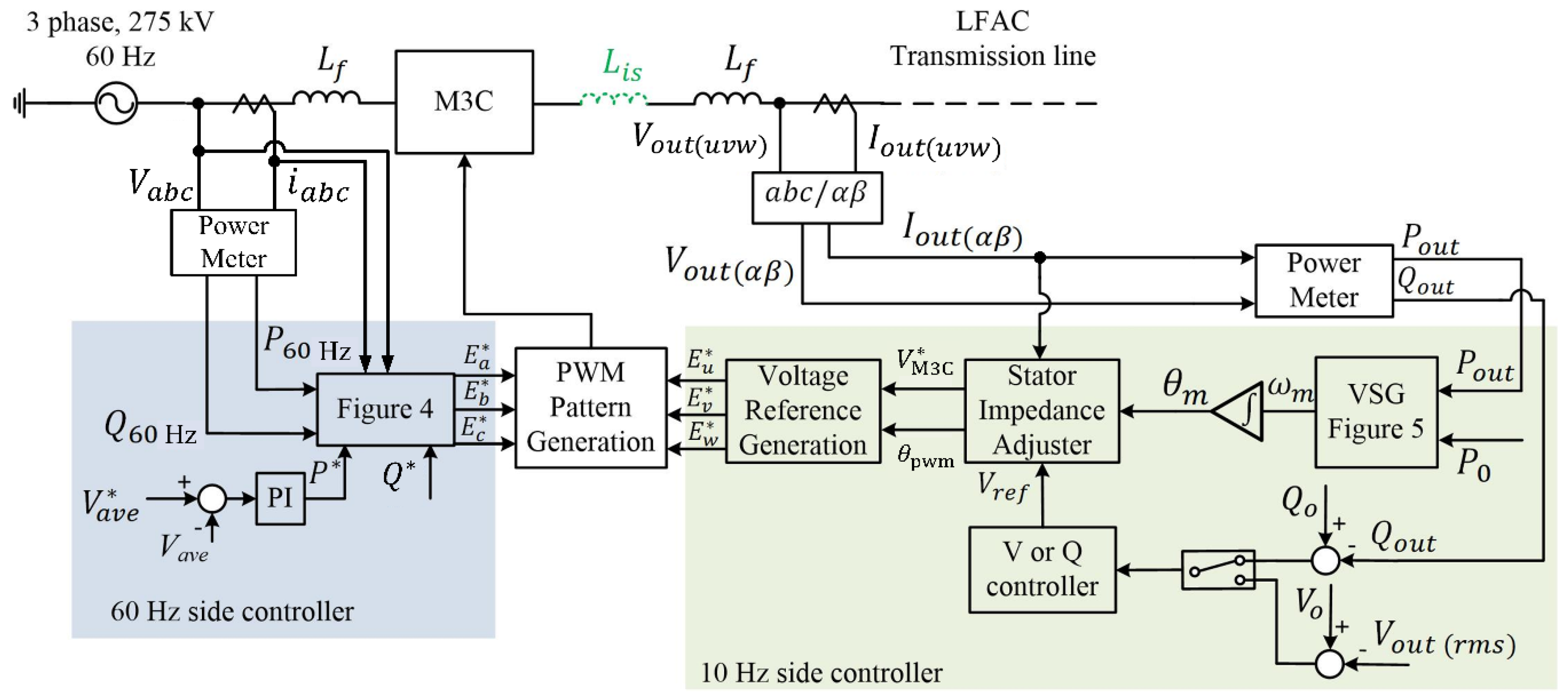
3.2. Overall Control Scheme of M3C

Figure 3 shows the overall control scheme of the M3C. The control scheme is divided into two parts; the input side (60 Hz side) conventional control part based on dq coordination frame, and the output side (10 Hz side) control part based on VSG control. The Input side control (60 Hz side) composed of outer and inner controllers. The outer controller is shown on the left hand side of Figure 4, which controls the input active and reactive power ($P_{60Hz}$, and $Q_{60Hz}$) using a proportional and integral (PI) controller to produce the dq axis reference currents $i_d^{*}$ and $i_q^{*}$ according to

$$i_d^{*}=\left(k+\frac{k_i}{s}\right)\frac{\left(P^{*}-P_{60Hz}\right)}{v_d}$$

(1)

$$i_q^{*}=\left(k+\frac{k_i}{s}\right)\frac{\left(Q^{*}-Q_{60Hz}\right)}{v_d}$$

(2)

The inner current controller (on the right-hand side of Figure 4) tries to track the reference currents using a proportional gain. This controller provides the voltage vector references $v_{d 60Hz}^{*}$ and $v_{q 60Hz}^{*}$ as follows

$$v_{d 60Hz}^{*}=k_d\left(i_d^{*}-i_d\right)-\omega L{i}_q+v_d$$

(3)

$$v_{q 60Hz}^{*}=k_q\left(i_q^{*}-i_q\right)+\omega L{i}_d+v_q$$

(4)

The voltage vector references are transformed to a three phase-to-neutral values $E_{abc}^{*}$ using an inverse park transformation with a phase-locked-loop (PLL).

It is noteworthy to mention that each H-bridge cell contains a capacitor which acts as a dc voltage source, and cell capacitor voltage must be kept almost constant around its given reference value. If this voltage value changes, it affects the output voltage of the low-frequency side as well as harmonic waveforms. Therefore, a capacitor average voltage deviation ΔV_ave control loop is employed to calculate the reference power command for the input side (60 Hz side) automatically by using the capacitor average voltage deviation and a PI controller. The capacitor average voltage V_ave is calculated from all the H-bridge cell capacitor voltages using (5),

$$V_{ave}=\frac{1}{N}{\displaystyle \sum }_{i=1}^N{V}_{cap\_i}$$

(5)

where $V_{cap\_i}$ is the capacitor voltage of the i_th cell and N is the total number of cells. A three phase-to-neutral voltage references are obtained through an inverse dq transformation as shown in Figure 4.

To determine pulse width modulation (PWM) pattern from the voltage references, space vector pulse-width modulation (SVPWM) control scheme is used. The capacitor in each H-bridge cell is regarded as a voltage source and various line-to-line voltages can be realized by the combination of the output voltages of these cells [32].

The 10 Hz-side controller is implemented by using the VSG control system, which is divided into two parts, active power control and reactive power or output voltage control. A detailed VSG control system is discussed in Section 4. Finally, the phase angle θ_m obtained from the VSG control is used to form the three reference phase voltages in the SVPWM.

4. VSG Control

The VSG control consists of two parts, the virtual inertia part based on the swing equation and the governor control part based on ω−P droop characteristic for deciding the mode of operation of the MT-LFAC system.

4.1. Active Power Control

The VSG control is used to control the amount and direction of the active power, and to synchronize, and stabilize the frequency among the terminals. The VSG control scheme that is used here is shown in Figure 5. The VSG control scheme comprises the swing equation, governor, and damping units. The swing equation of VSG is

$$P_{in}-P_{out}+P_d=J{\omega }_0\frac{d{\omega }_m}{dt}$$

(6)

where ω_m is the virtual rotating angular frequency, ω₀ is the nominal frequency, and $P_{in}$, $P_{out}$, P_d are the virtual shaft power produced by the governor control, the output power of the low frequency side, and the damping power, respectively. J is the moment of inertia of rotating mass, which is determined as

$$J=\frac{M{S}_{base}}{{\omega }_0^2}$$

(7)

where M is the inertia time constant, $S_{base}$ is the rated power of each respective terminal.

The damping power P_d is generated by the state feedback control method [33] as follows

$$P_d=-k_{x\omega }\left({\omega }_m-{\omega }_0\right)-k_{xP}\frac{1}{1+T_{f}s}{P}_{out}-k_{xi}\frac{1}{s}{P}_d$$

(8)

where $k_{x\omega }$, $k_{xp}$, and $k_{xi}$ are the feedback gains of virtual rotor frequency, output active power, and integral term of P_d, and $T_f$ is the time constant of the low-pass filter (LPF), that is calculated based on

$$T_f=\frac{1}{2\pi f_f}$$

(9)

where, $f_f$ is the cut off frequency. We chose $f_f$ = 10 Hz in order to attenuate the 2ω_m ripples. This damping method technique is chosen because it can provide a fast response to power command change, and it can allow adding an LPF to filter the measured active power $P_{out}$ in order to attenuate the ripples caused by the unbalance in the output voltage and/or current in the LFAC side. These ripples will affect the output power quality since they will enter the VSG control block. Moreover, we can avoid using the phase locked loop (PLL) for detecting grid frequency, which is used in some previous works [34,35]. All values are shown in

Table 1. Simulation parameters.

Common Parameters
Parameter	Value	Parameter	Value
$V_{base}$	275 kV	$X_{10 Hz side}$	0.016 pu
$f_{in}$	60 Hz	Terminal 1 VA $S_{base1}$	200 MVA
$f_{out}$	10 Hz	Terminal 2 VA $S_{base2}$	120 MVA
$X_{60 Hz side}$	0.1 pu	Terminal 3 VA $S_{base3}$	80 MVA
Modular Multilevel Matrix Converter (M3C) Parameters
Parameter		Value
Sampling frequency		2 kHz
Capacitor voltage		128 kV
Cell capacitor Arm inductor		470 μf 128 μH
Virtual Synchronous Generator (VSG) Parameters
$V_{base}$	275 kV	$\rho$	0.29203
$P_{0\_pu}$	1.0 pu	$k_{xp}$	1.0
ω0	62.831 rad/s	$k_{x\omega }$	91.4140 pu
$k_{p\_pu}$	20 pu	$k_{xi}$	8.8522 s−1
M	8 s	$T_f$	0.0159 s
Automatic Reactive Power (AQR) and Automatic Voltage Regulator (AVR) PI Controller Parameters
$K_p$		0.001 pu
$K_i$		0.5 s
Transmission Line Parameters
Cross-linked polyethylene (XLPE) Single core land cable
Cross section		500 mm2
L		0.61 mH/km
C		0.14 μf/km
R		0.0255 Ω/km

*The pu value in this table are based on self-power rating of each terminal.

. From (8), it can be noticed that the integral term of P_d exists, and this will force P_d = 0 in the steady state. By rearranging (6), the virtual mechanical frequency can be rewritten as (10)

$${\omega }_m=\frac{1}{J{\omega }_0}\int \left(P_{in}-P_{out}+P_d\right)dt$$

(10)

The obtained virtual angular frequency ω_m is then integrated to generate the phase angle θ_m to be utilized afterwards by the inner controller of the M3C. The parameter design of the VSG control part is shown in [28,33].

4.2. Governor Control and $\omega$−P Droop Characteristics

The governor control part of the VSG, shown in Figure 5, is based on the $\omega -P$ droop characteristic. It is preferable to use the $\omega -P$ droop control especially when the system is highly inductive like the traditional synchronous generator [36]. From Figure 5, it can be noticed that there is a selector to decide the reference power term of the governor droop control. If P₀ is selected, the governor will operate in commanded mode. On the other hand, if $P_{out}$ is selected (where, $P_{out}$ is the low frequency side online output power), a frequency restoration mode of operation will be performed.

The governor droop characteristic control has a conventional droop and reversed droop, as shown in Figure 6. In the commanded mode, the virtual shaft power $P_{in}$ is produced by the governor control as

$$\begin{array}{c}{P}_{in}=P_0-k_p\left({\omega }_m-{\omega }_0\right)\left(\mathrm{conventional}\right)\\ P_{in}=P_0+k_p\left({\omega }_m-{\omega }_0\right)\left(\mathrm{reverse}\right)\end{array}$$

(11)

where $P_0$ is the commanded value of active power, which is set in per unit, and ω₀ is the nominal frequency? $k_p$ is the droop coefficient which is proportional to the power rating of each corresponding terminal and is determined as follows:

$$k_{p\_pu}=\frac{k_p{\omega }_0}{S_{base}}$$

(12)

where, $S_{base}$ is the power rating of each terminal. The adopted value $k_{p\_pu}=20$ shown in Table 1 allows a maximum 5% frequency deviation during a 1.0 pu power transition, which is a typical value in the power system [33,36,37].

According to the droop characteristic illustrated by Figure 6, Terminals 2 and 3 are assigned by a reverse droop control, compared to conventional droop in Terminal 1. This is achieved by assigning the droop coefficient $k_p$ with a different sign. In Figure 6, the subscript $T_i$ indicates Terminal i (i = 1, 2, 3). In a multi-terminal system, the terminal designed to be the receiver can be assigned by a reverse droop while the terminal designed to be the sender can be assigned with the conventional droop control. It is noteworthy to mention that the power flow can also be from the receiver to the sender without any modification of droop characteristic. The $k_p$ of all terminals remains unchanged throughout the simulation presented in Section 5.

From Figure 5, when the frequency restoration mode of operation is selected, $P_0$ is substituted by $P_{out}$, thus Equation (11) becomes

$$\begin{array}{c}{P}_{in}=P_{out}-k_p\left({\omega }_m-{\omega }_0\right) \left(\mathrm{conventional}\right)\\ P_{in}=P_{out}+k_p\left({\omega }_m-{\omega }_0\right) \left(\mathrm{reverse}\right)\end{array}$$

(13)

By substituting (13) in (10) we get

$$\begin{array}{c}{\omega }_m=\frac{1}{J{\omega }_0}\int \left(P_{out}+k_p\left({\omega }_m-{\omega }_0\right)-P_{out}+P_d\right)dt\\ =\frac{1}{J{\omega }_0}\int \left(k_p\left({\omega }_m-{\omega }_0\right)+P_d\right)dt\end{array}$$

(14)

According to (14), it can be noticed that in the steady state, we have $k_p\left({\omega }_m-{\omega }_0\right)+P_d=0$. As $P_d$ = 0 in the steady state [33], thus ω_m = ω₀. That is to say, the proposed control scheme allows the operator to smoothly restore the frequency in an MT-LFAC system. Unlike the previous reports that mostly worked on the supervisory upper-level control, the present paper is focused on the entire control system to reach the assigned control objectives in the MT-LFAC system. For the terminals operating in commanded mode, as ω_m = ω₀, from (11), $P_{in}=P_0$. That is to say, the output power will follow the command accurately.

Finally, owing to the governor control, two objectives can be fulfilled. First, the system can operate under frequency restoration mode, by that it senses the frequency variation of the network and decides the reference active power as given in (13). Secondly, based on (14), the frequency deviation restoration can be achieved.

4.3. Reactive Power and Voltage Control

In this model, the approaches taken to control the output voltage and reactive power are similar to the conventional ones in the HVAC system. Terminal 1 is set as a slack bus which is assigned to control the voltage. Terminals 2 and 3 are aimed to control the reactive power by changing the output voltage. In other words, Terminal 1 is V-controlled (PV bus), whereas Terminals 2 and 3 are Q-controlled (PQ buses).

The reactive power control aims to control the low frequency side output voltage profile which minimizes the active power losses of each terminal. This is accomplished by using an AVR with low frequency side output voltage feedback or an AQR with low frequency side output reactive power feedback as they are shown in the left side of Figure 7. A selector is used in order to choose the method for controlling either the voltage or the reactive power. Terminal 1 is chosen to be responsible for controlling the output voltage by using AVR control. At the same time, Terminals 2 and 3 control the required reactive power to be provided for the transmission lines by using the AQR control. The AQR is a fixed type controller, which can follow a given command. The command of AQR in each terminal is set to provide reactive power consumed in the transmission line connected to this terminal, in order to minimize the reactive power in the LFAC system.

For the AQR control, because no reactive power transmission between the terminals is required in the MT-LFAC system, it is calculated and commanded in order to ensure the lowest possible losses, thus, a fixed reactive power value calculated from the reactance and capacitance values of the transmission line. After determining the reactive power for each terminal, the reference reactive power command can be set accordingly, which is shown by the AQR control block Q₀ in Figure 7. From this figure, the resulted voltage $V_{ref}$ is the RMS reference voltage, which will be updated by the virtual impedance control block.

4.4. Stator Impedance Adjuster

In this subsection, it is important to discuss about the low frequency transmission line X/R issue. Due to the low frequency used, the obtained X/R ratio will be 6 times smaller than that of the 60 Hz for a given rated voltage level, in which it is 1.5 in our case [38,39]. Therefore, the system will become less inductive. To fix the negative impact of this fact, a virtual stator reactance is introduced to the VSG control in order to increase the total reactance of each terminal in order to avoid the coupling between P and Q. In [35], for a 60 Hz network, the total impedance X^* is set to 0.7 pu. In our work, the frequency difference is taken as criteria, thus the total impedance X^* is fixed at 0.1 pu, which is sufficient to make a larger X/R ratio, hence, to make the system inductive again. The total reactance X^* in pu according to self-power rating is calculated as

$$X^{*}=\frac{X{S}_{base}}{V_{base}^2}=\frac{{\omega }_0\left(L_{ls}+L_f+L_{line}\right)S_{base}}{V_{base}^2}=0.1\mathrm{pu}$$

(15)

where, $L_{ls}$ is the virtual stator inductance, $L_f$ and $L_{line}$ are the inductance of the L filter and the transmission line, respectively. From (15), $L_{ls}$ is calculated as 0.089 pu for each terminal. Then, the reference voltage obtained from the AVR/AQR will be converted into a stationary frame, this reference voltage will be updated according to the multiplication of the virtual stator inductor with the output current. Here, a stationary-frame based virtual impedance is applied owing to its simplicity and PLL-free nature. Then, the new reference voltage $V_{M3C}^{*}$ will be realized and used for the SVPWM of the M3C.

4.5. On Real-World Applicability of the Proposed Approach

As shown in Figure 2, the M3Cs, as a promising topology for high-voltage high-power applications, use a high number of switches and thus are more complex in comparison with conventional converters. This issue may call into question on the applicability of the proposed control methodology. As emphasized in Section 1, because of the numerous advantages at high voltage and power levels, they are widely used in various applications in the last two decades [40]. Due to their modular structure, they offer easy scalability, high-quality output waveforms, and superior availability. Due to low-loss operation, high redundancy, and high reliability, the M3C could also be extremely attractive for high voltage transmission systems compared to state-of-the-art converters.

In summary, because of the following reasons the M3C application in the proposed control scheme for the electrical energy transmission systems is explainable:

(1)

Despite the high number of power cells required by the M3C, its constructive characteristics allow low-frequency operation with low circulating current requirements. Moreover, the above-mentioned advantages and its grid-code compliance performance are examined among the other high-power converter topologies in some real-world applications such as high-power wind energy and motor drive systems [41,42,43].

(2)

Unlike a low voltage small grid, a power energy transmission system is a bulk costly system with expensive components and installation process. Therefore, improving the control/operation performance of this system, even with complex devices/converters and control mechanisms are allowed. Advantages of the applied M3C-based control scheme such as enhancing dynamic performance and reducing the line losses in a high voltage/power system can compensate the higher degree of complexity of the used converters.

(3)

Due to the symmetrical structure of the multilevel matrix converter, both step-up and step-down of voltage magnitude can be easily done. This feature causes us to use the converter without transformer, and the transformer-less operation; in addition to increase of efficiency, flexibility, scalability, modularity and reliability, this leads to a lower installation and operation costs in a power transmission system.

(4)

It is shown that the M3C can present the fault tolerance property, i.e., after a branch failure, the nine branch M3C can be reduced to operate as a six-branch Hexverter [44]. Furthermore, the M3C employs inductive elements on both sides and then requires five conducting branches at any instant, which means indeed that the number of under control switches in the performed system is reduced to 80.

(5)

Although the M3Cs are still under research and development, they have already found successful industrial applications, and many new contributions and new commercial topologies have been reported in the last few years [40]. Therefore, they can be considered a mature and proven technology. Some reported applications are addressed in [17,40,41,42,43,44], and M3Cs for these applications are commercially offered by a growing group of companies in the field [45].

(6)

The M3C is the only converter system that effectively increases the power rating of the converter. This topology elevates the voltage by the series connection of power modules. Of course, its high level of complexity must be responded by performing an effective/advanced control design methodology and a sophisticated control structure such as the one proposed (using VSG) in our manuscript.

5. Simulation Results

This section demonstrates the performance of the control system chosen to operate the MT-LFAC system and discusses different case studies applied to verify the proposed control approach used for the introduced case study. Furthermore, this section evaluates the VSG control scheme after transient events including the change of the power command and a power flow reversal, in addition to transition of switching modes. The power flow algorithm and the case studies are implemented in PSCAD/EMTDC software environment.

The MT-LFAC system composed of three terminals, as shown in Figure 1, was used for simulation. All terminals employ an M3C and a VSG control system. The terminals are connected via 200 km modeled as $\pi$–circuit transmission line. The transmission power cable parameters and other simulation parameters are shown in Table 1. The values of the PI parameters were manually tuned in per unit based on respective power or voltage ratings of each terminal.

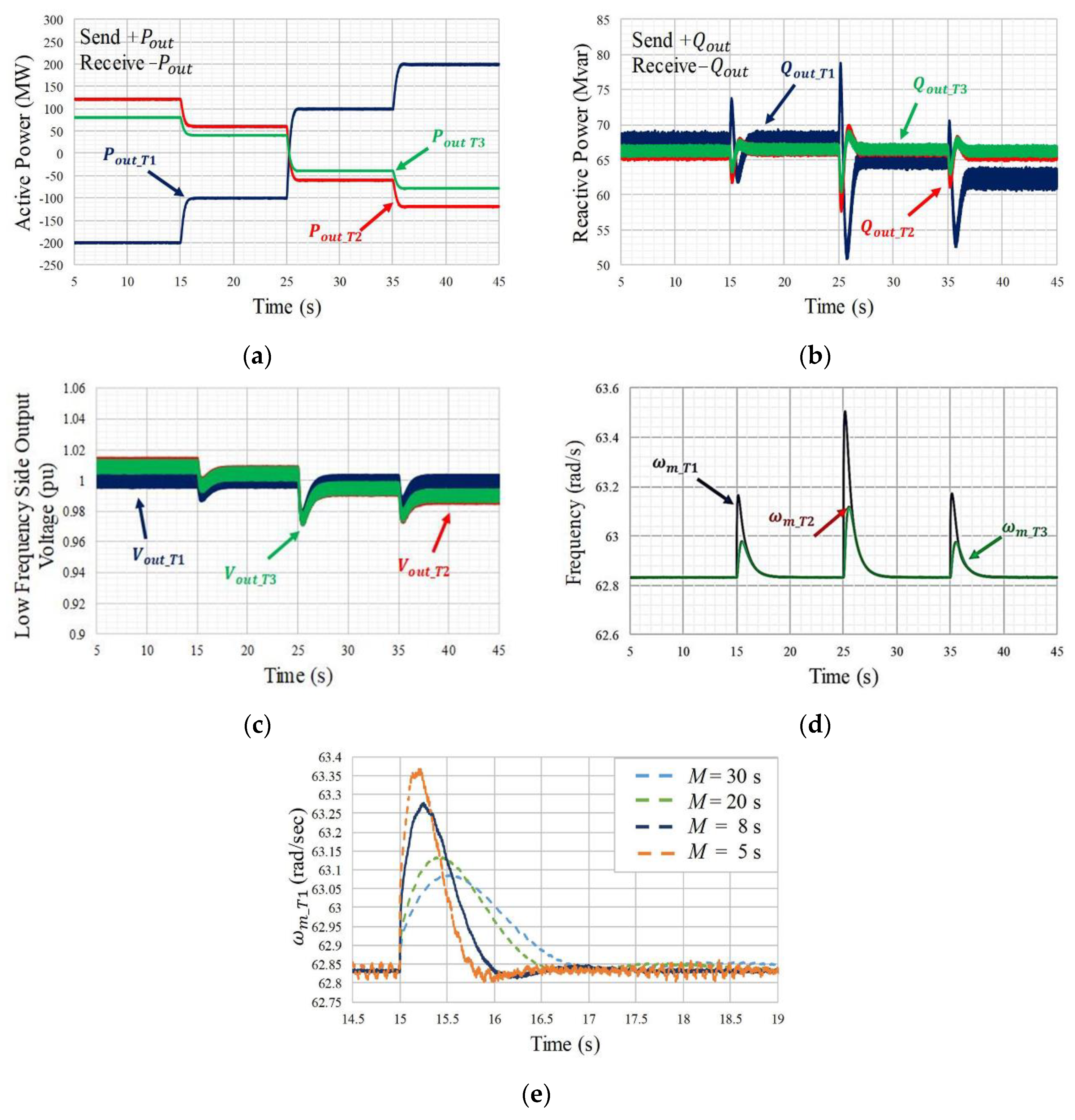
5.1. Case 1: Terminal 1 Commanded Mode, Terminals 2 And 3 Frequency Restoration Mode

In this case, Terminals 2 and 3 were in frequency restoration mode, and are controlled following a frequency variation in Terminal 1. We chose this case instead of a full commanded mode system in order to confirm the VSG control robustness. This is done by setting a predefined reference power to the governor part of Terminal 1.

Figure 8a demonstrates this case study, where the active power of three terminals are shown. The positive part indicates that the power is being sent. Terminals 1, 2 and 3 were designed as 200 MVA, 120 MVA and 80 MVA, respectively. The scenario of command change sequence is as follows; at 0–15 s Terminal 1 is commanded to receive 200 MW from Terminals 2 and 3. At 15 s, Terminal 1 changes its command value to receive 100 MW. At 25 s, Terminal 1 starts to send 100 MW power instead of receiving it. Finally, at 35 s, Terminal 1 sends 200 MW to the Terminals 2 and 3. From Figure 8a and according to the described scenario, the proposed control for the MT-LFAC system based on the governor $\omega -P$ droop control has been successfully performed with sharing power to Terminal 1 properly according to the power ratings of Terminals 2 and 3.

Figure 8b,c show the reactive power and output voltage responses. The positive part indicates that the leading reactive power is provided by each terminal for the transmission line. Compared to the 50 Hz or 60 Hz conventional transmission lines, and according to

Table 2. Reactive power comparison.

Transmission Line Type	${\mathit{Q}}_{\mathit{o}\mathit{u}\mathit{t}\_\mathit{T}1}$ (Mvar)	${\mathit{Q}}_{\mathit{o}\mathit{u}{\mathit{t}}_{\mathit{T}2}}$ (Mvar)	${\mathit{Q}}_{\mathit{o}\mathit{u}{\mathit{t}}_{\mathit{T}3}}$ (Mvar)
Low Frequency AC (LFAC)	64.472	65.765	66.168
High Voltage AC (HVAC)	385.895	393.656	396.077

, the numerical analysis shows that the reactive power was reduced almost 6 times in the case of the LFAC transmission system. Thus, by using the LFAC transmission, the main advantage of reduced losses can be achieved. Moreover, it was decided for Terminal 1 to control the output voltage whereas Terminals 2 and 3 are responsible of controlling the reactive power. Therefore, from Figure 8c the output voltage of Terminal 1 was kept constant due to the AVR control. On the other hand, both voltages of T2 and T3 have similar deviations in voltage since they are controlled by AQR, thus, their terminal voltage is not directly controlled. However, the voltage sag is almost less than 3%, which is acceptable.

Figure 8d shows the virtual angular frequency of each terminal at the 10 Hz side. It is seen that the angular frequency deviates during each dynamic state and returns to its steady state after a short time. The settling time is almost the same, and it depends on the inertia constant M. Figure 8e demonstrates the reason for choosing the inertia constant M. From the figure, it can be noticed that by increasing M the overshoot will be smaller with a longer settling time. When M is decreased, with a shorter settling time, overshoot becomes bigger, and larger ripples appeared in the response. Therefore, M = 8 s is chosen considering a tradeoff between the transient performance (e.g., overshoot, settling time, and ripples).

In addition, in order to better interpret the performance of the M3C in the MT-LFAC system, simulation results are shown in Figure 9 that demonstrate Terminal 1 M3C operation. Figure 9a,b represent the 60 Hz side active and reactive power, and capacitor average voltage waveforms, respectively. After the transients are applied on the low frequency side, the controllers of each corresponding M3C succeed in keeping the power balance between the input and output sides. This resulted in a constant capacitor average voltage waveform with only a small deviation (less than 0.5%) is obtained when the power command changes. Moreover, the power flow pattern on the 60 Hz side automatically follows the power flow change on the low frequency side considering that the active power command of the 60 Hz side is set indirectly based on capacitor average voltage deviation. Figure 9c,d show the 60 Hz and low frequency sides sinusoidal current and voltage zoom in waveforms when the power reversal occurs at 25 s, which also follow the power flow patterns. It is clear that the M3C succeed in providing improved sinusoidal waveforms.

5.2. Case 2 Terminals 1 and 2 Commanded Mode, Terminal 3 Frequency Restoration Mode

In this case, the proposed system is tested in order to confirm the flexibility of the proposed control system. Hence, Terminals 1 and 2 are in commanded mode whereas Terminal 3 is in frequency restoration mode. The dynamic scenario is divided into two parts. Referring to Figure 10a, until 10 s, the commanded values to Terminals 1 and 2 are −150 MW (receiving) and 90 MW (sending), respectively. After 10 s, Terminal 2 power is increased to be 100 MW. As a result, Terminal 3 power is decreased based on the frequency restoration mode control. Finally, at 20 s, a full power reversal occurs. Hence, Terminal 1 starts to send the 150 MW while Terminals 2 (receives 100 MW) and 3 become receivers. Assumed operation can be successfully performed from Figure 10a.

Figure 10b,c show the reactive power and the output voltage responses, respectively. The controller is the same as in Case 1. The difference in the AQR control is the reference command for the reactive power, which is also affected by the power change of the corresponding terminals. Moreover, since the AVR is used for controlling the voltage of Terminal 1, the reactive power of this terminal is not controlled at a specific value, thus it is dependent on the rest of the network. Oppositely, Terminals T2 and T3 are controlled by AQRs, thus their reactive power tracks respective reactive power command strictly, except transient condition.

Figure 10d, shows the output angular frequency of each terminal. Similar to Case 1, the frequency deviates after each power dynamic state and is promptly recovered due to the reverse droop control of the terminals against each other. Moreover, from the figure, at each dynamic state, firstly, the frequency of the master terminal changes. In response, the droop control of the terminal frequency restoration mode synthesizes this event and changes its frequency. Terminal 3 changes its power accordingly without causing any steady-state frequency deviation.

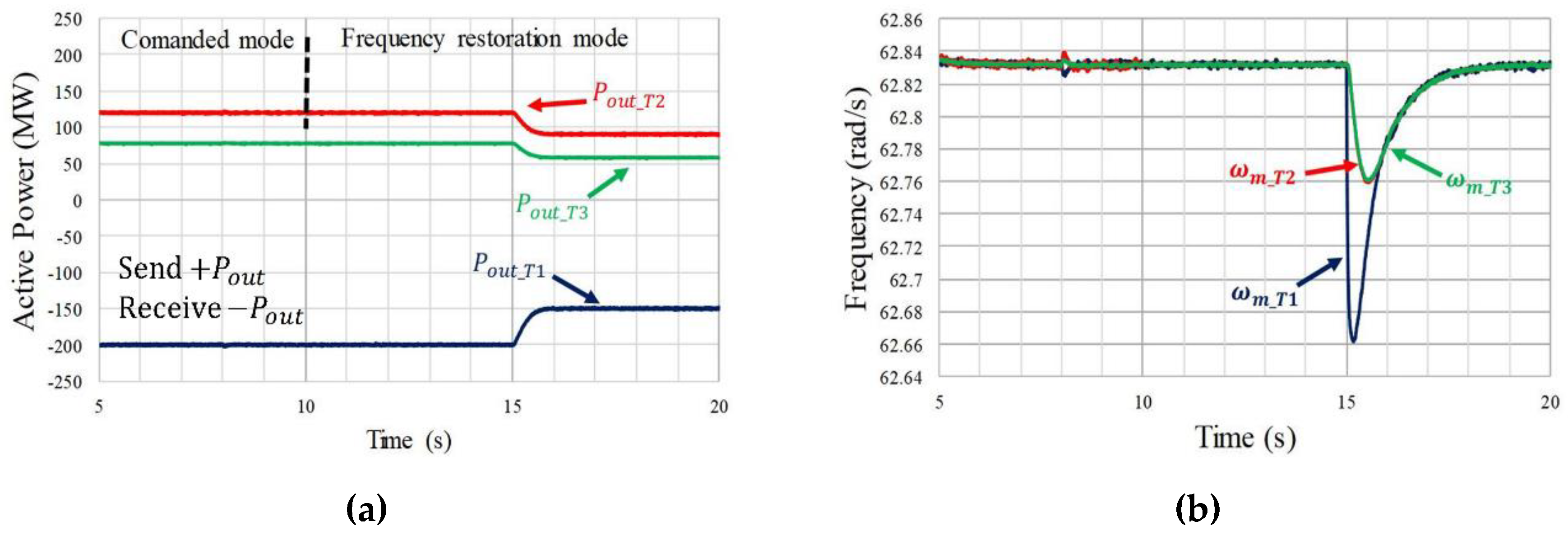
5.3. Case 3: Terminal 2 Switching from Commanded Mode To Frequency Restoration Mode

In this case, the proposed system is tested in a scenario including control mode transition. In this scenario as depicted in Figure 11a, first, both Terminals 1 and 2 are operated in commanded mode based on their respective power ratings, and Terminal 3 operates in frequency restoration mode. Then, at t = 10 s, the switch of Terminal 2 Figure 5, changes from commanded mode to frequency restoration mode. It can be seen, during this mode transition, the power sharing acts smoothly and remains constant. Thus, the VSG was able to guarantee a proper power sharing without any dedicated communication channel. Thus, the scenario becomes the same as in Case 1 when Terminal 1 controls the power flow of the entire system by its commanded value. At t = 15 s, the command of Terminal 1 changes to receive 175 MW instead of 200 MW and based on the frequency restoration mode in Terminals 2 and 3, the power command was properly accommodated.

Figure 11b shows the output angular frequency of each terminal. It can be noticed that there is even no frequency deviation during the transition of the mode switching of Terminal 2. Similar to Case 1, the frequency deviates after 15 s and is promptly recovered due to the reverse droop control of the terminals against each other.

The system response shown in Figure 11 demonstrates that, unlike the conventional frequency restoration method, the proposed frequency restoration mode can be started at different instants while keeping a reasonable power allocation.

6. Conclusions

In this paper, we proposed a control scheme to form a multi-terminal low-frequency ac (MT-LFAC) system as an alternative solution to both multi-terminal high voltage DC (MT-HVDC) and high voltage AC (HVAC) systems in order to provide long distance transmission to interconnect remote power systems. Characteristics of the proposed system are studied, and the obtained results are summarized as follows:

(1)

The modular multilevel matrix converter (M3C) was proposed for frequency conversion between nominal frequency (50 or 60 Hz) and low frequency (50/3 and/or 60/3 Hz) in order to obtain higher power quality and lower power conversion losses.

(2)

Application of virtual synchronous generator (VSG) control in 10 Hz side was proposed in order to autonomously control active and reactive power and voltage of each terminal and maintaining the frequency stable in the steady-state.

(3)

The VSG control used in this work has succeeded on enabling the M3Cs to behave like synchronous generators to construct the MT-LFAC network.

(4)

Autonomous frequency restoration is realized by the proposed frequency restoration mode and the problem of the low X/R ratio in LFAC is solved by virtual impedance control.

(5)

Operation of the proposed system was demonstrated by the computer simulation using PSCAD/EMTDC software. Smooth operation during changes of power reference values were achieved.

(6)

The control scheme proposed for the MT-LFAC system has proved its flexibility, and its ease of implementation. Thus, the multiterminal system can be easily extended to more terminals without altering the controller coefficients and/or parameters since they are in per unit values. The only point that needs to be considered is deciding the role of power flow, for example; each terminal capacity, sending vs. receiving groups of terminals, and the total amount of the power that needs to be accommodated.

To investigate the effectiveness of the proposed control scheme and to minimize the existing gap between simulation environment and practice, in the present research, the detailed dynamics for the system under study are considered, and high precise nonlinear models for the components and accurately defined parameters in the proposed control framework are employed. However, since the experimental test is the ultimate approach for validation of a new control strategy, this issue can be considered a future step for the present research work. Further research steps can be focused on coordination control of M3C with AC grids in order to reduce the impact on AC grids, and evaluation of losses of the system are considered.

References

1. Belda, N.A.; Plet, C.A.; Smeets, R.P.P. Analysis of Faults in Multiterminal HVDC Grid for Definition of Test Requirements of HVDC Circuit Breakers. IEEE Trans. Power Deliv. 2018, 60, 403–411. [Google Scholar] [CrossRef]
2. Chen, J.; Dou, Y.; Li, Y.; Li, J.; Li, G. A Transient Fault Recognition Method for an AC-DC Hybrid Transmission System Based on MMC Information Fusion. Energies 2017, 10, 23. [Google Scholar] [CrossRef] [Green Version]
3. Bevrani, H.; Watanabe, M.; Mitani, Y. Power System Monitoring and Control; IEEE-Wiley press: New York, NY, USA, 2014. [Google Scholar]
4. Bozhko, S.V.; Blasco-Giménez, R.; Li, R.; Clare, J.C.; Asher, G.M. Control of offshore DFIG-based wind farm grid with line-commutated HVDC connection. IEEE Trans. Energy Convers. 2007, 22, 71–78. [Google Scholar] [CrossRef]
5. Wang, X.; Wang, X. Feasibility study of fractional frequency transmission system. IEEE Trans. Power Syst. 2013, 11, 962–967. [Google Scholar] [CrossRef]
6. Pichetjamroen, A.; Ise, T. Power Control of Low Frequency AC Transmission Systems Using Cycloconverters with Virtual Synchronous Generator Control. Energies 2017, 10, 34. [Google Scholar] [CrossRef] [Green Version]
7. Pichetjamroen, A.; Ise, T. A Proposal on Low Frequency AC Transmission as a Multi-Terminal Transmission System. Energies 2016, 9, 687. [Google Scholar] [CrossRef] [Green Version]
8. Liu, S.; Wang, X.; Ning, L.; Wang, B.; Lu, M.; Shao, C. Integrating Offshore Wind Power Via Fractional Frequency Transmission System. IEEE Trans. Power Deliv. 2017, 32, 1253–1261. [Google Scholar] [CrossRef]
9. Nguyen, Q.; Todeschini, G.; Santoso, S. Power Flow in a Multi-Frequency HVac and HVdc System: Formulation, Solution, and Validation. IEEE Trans. Power Syst. 2019, 34, 2487–2497. [Google Scholar] [CrossRef]
10. Ruddy, J.; Meere, R.; O’Donnell, T. Low Frequency AC transmission as an alternative to VSC-HVDC for grid interconnection of offshore wind. In Proceedings of the 2015 IEEE Eindhoven Power Tech, Eindhoven, The Netherlands, 29 June–2 July 2015. [Google Scholar]
11. Fischer, W.; Braun, R.; Erlich, I. Low frequency high voltage offshore grid for transmission of renewable power. In Proceedings of the 3rd IEEE PES Innovative Smart Grid Technolgies Europe (ISGT Europe), Berlin, Germany, 14–17 October 2012. [Google Scholar]
12. Cho, Y.; Cokkinides, C.J.; Meliopoulos, A.P. Time domain simulation of a three-phase cycloconverter for LFAC transmission systems. In Proceedings of the IEEE PES Transmission and Distribution Conference and Exposition (PES T&D), Orlando, FL, USA, 7–10 May 2012. [Google Scholar]
13. Chen, H.; Johnson, M.H.; Aliprantis, D.C. Low-Frequency AC Transmission for Offshore Wind Power. IEEE Trans. Power Deliv. 2013, 28, 2236–2244. [Google Scholar] [CrossRef]
14. Kawamura, W.; Chen, K.; Hagiwara, M.; Akagi, H. A Low-Speed, High-Torque Motor Drive Using a Modular Multilevel Cascade Converter Based on Triple-Star Bridge Cells (MMCC-TSBC). IEEE Trans. Ind. Appl. 2015, 51, 3965–3974. [Google Scholar] [CrossRef]
15. Liu, S.; Wang, X.; Meng, Y.; Sun, P.; Luo, H.; Wang, B. A Decoupled Control Strategy of Modular Multilevel Matrix Converter for Fractional Frequency Transmission System. IEEE Trans. Power Deliv. 2017, 32, 2111–2121. [Google Scholar] [CrossRef]
16. Ludois, D.C.; Reed, J.K.; Venkataramanan, G. Hierarchical Control of Bridge-of-Bridge Multilevel Power Converters. IEEE Trans. Ind. Electron. 2010, 57, 2679–2690. [Google Scholar] [CrossRef]
17. Kouro, S.; Malinowski, M.; Gopakumar, K.; Pou, J.; Franquelo, L.; Wu, B.; Rodriguez, L.; Perez, M.; Leon, J. Recent advances and industrial applications of multilevel converters. IEEE Trans. Ind. Electron. 2010, 57, 2553–2580. [Google Scholar] [CrossRef]
18. Perez, M.A.; Bernet, S.; Rodriguez, J.; Kouro, S.; Lizana, R. Circuit Topologies, Modeling, Control Schemes, and Applications of Modular Multilevel Converters. IEEE Trans. Power Electron. 2015, 30, 4–17. [Google Scholar] [CrossRef]
19. Kouro, S.; Rodriguez, J.; Wu, B.; Bernet, S.; Perez, M. Powering the Future of Industry: High-Power Adjustable Speed Drive Topologies. IEEE Ind. Appl. Mag. 2012, 18, 26–39. [Google Scholar] [CrossRef]
20. Nami, A.; Liang, J.; Dijkhuizen, F.; Demetriades, G.D. Modular multilevel converters for HVDC applications: Review on converter cells and functionalities. IEEE Trans. Power Electron. 2015, 30, 18–36. [Google Scholar] [CrossRef]
21. Wang, K.; Li, Y.; Zheng, Z.; Xu, L. Voltage balancing and fluctuation suppression methods of floating capacitors in a new modular multilevel converter. IEEE Trans. Ind. Electron. 2013, 60, 1943–1954. [Google Scholar] [CrossRef]
22. Moranchel, M.; Bueno, E.; Sanz, I.; Rodríguez, F.J. New Approaches to Circulating Current Controllers for Modular Multilevel Converters. Energies 2017, 10, 86. [Google Scholar] [CrossRef]
23. Zhang, L.; Harnefors, L.; Nee, H.P. Power-synchronization control of grid-connected voltage-source converters. IEEE Trans. Power Syst. 2010, 25, 809–820. [Google Scholar] [CrossRef]
24. Zhong, Q.C.; Weiss, G. Synchronverters: Inverters that mimic synchronous generators. IEEE Trans. Ind. Electron 2011, 58, 1259–1267. [Google Scholar] [CrossRef]
25. Alipoor, J.; Miura, Y.; Ise, T. Power system stabilization using virtual synchronous generator with alternating moment of inertia. IEEE J. Emerg. Sel. Top. Power Electron 2015, 3, 451–458. [Google Scholar] [CrossRef]
26. Zhang, L.; Harnefors, L.; Nee, H.P. Modeling and control of VSCHVDC links connected to island systems. IEEE Trans. Power Syst. 2011, 26, 783–793. [Google Scholar] [CrossRef]
27. Bevrani, H.; Fracois, B.; Ise, T. Microgrid Dynamics and Control; Wiley: Hoboken, NJ, USA, 2017. [Google Scholar]
28. Liu, J.; Miura, Y.; Ise, T. Comparison of Dynamic Characteristics Between Virtual Synchronous Generator and Droop Control in Inverter-Based Distributed Generators. IEEE Trans. Power Electron. 2016, 31, 3600–3611. [Google Scholar] [CrossRef]
29. Zhu, J.; Booth, C.D.; Adam, G.P.; Roscoe, A.J.; Bright, C.G. Inertia Emulation Control Strategy for VSC-HVDC Transmission Systems. IEEE Trans. Power Syst. 2013, 28, 1277–1287. [Google Scholar] [CrossRef] [Green Version]
30. XLPE Land Cable Systems User’s Guide. Available online: https://library.e.abb.com/public (accessed on 2 July 2019).
31. Kammerer, F.; Kolb, J.; Braun, M. A novel cascaded vector control scheme for the modular multilevel converter. In Proceedings of the 37th Annual Conference of the IEEE Industrial Electronics Society (IECON), Melbourne, Australia, 7–10 November 2011. [Google Scholar]
32. Miura, Y.; Mizutani, T.; Ito, M.; Ise, T. Modular multilevel matrix converter for low frequency AC transmission. In Proceedings of the IEEE 10th International Conference on Power Electronics and Drive Systems (PEDS), Kitakyushu, Japan, 22–25 April 2013; pp. 1079–1084. [Google Scholar]
33. Liu, J.; Miura, Y.; Ise, T. Fixed-Parameter Damping Methods of Virtual Synchronous Generator Control Using State Feedback. IEEE Access 2016, 7, 99177–99190. [Google Scholar] [CrossRef]
34. Shintai, T.; Miura, Y.; Ise, T. Oscillation damping of a distributed generator using a virtual synchronous generator. IEEE Trans. Power Del. 2014, 29, 668–676. [Google Scholar] [CrossRef]
35. Liu, J.; Miura, Y.; Bevrani, H.; Ise, T. Enhanced Virtual Synchronous Generator Control for Parallel Inverters in Microgrids. IEEE Trans. Smart Grid 2017, 8, 2268–2277. [Google Scholar] [CrossRef]
36. Bevrani, H. Robust Power System Frequency Control, 2nd ed.; Springer: Berlin/Heidelberg, Germany, 2014. [Google Scholar]
37. Sakimoto, K.; Miura, Y.; Ise, T. Stabilization of a power system including inverter-type distributed generators by a virtual synchronous generator. Electr. Eng. Jpn. (Engl. Transl. Denki Gakkai Ronbunshi) 2014, 187, 7–17. [Google Scholar] [CrossRef]
38. Ngo, T.; Lwin, M.; Santoso, S. Steady-State Analysis and Performance of Low Frequency AC Transmission Lines. IEEE Trans. Power Syst. 2016, 31, 3873–3880. [Google Scholar] [CrossRef]
39. Tleis, N. Power Systems Modelling and Fault Analysis; Newnes Elsevier: Oxford, UK, 2008; pp. 616–618. [Google Scholar]
40. Du, S.; Dekka, A.; Wu, B.; Zargari, N. Modular Multilevel Converters: Analysis, Control, and Applications; Wiley-IEEE Press: Hoboken, NJ, USA, 2017. [Google Scholar]
41. Kawamura, W.; Hagiwara, M.; Akagi, H. Control and experiment of a modular multilevel cascade converter based on triple-star bridge cells. IEEE Trans. Ind. Appl. 2014, 50, 3536–3548. [Google Scholar] [CrossRef]
42. Baruschka, L.; Mertens, A. A new three-phase AC/AC modular multilevel converter with six branches in hexagonal configuration. IEEE Trans. Ind. Appl. 2013, 49, 1400–1410. [Google Scholar] [CrossRef]
43. Kawamura, W.; Hagiwara, M.; Akagi, H.; Tsukakoshi, M.; Nakamura, R.; Kodama, S. AC-Inductors design for a modular multilevel TSBC converter, and performance of a low-speed high-torque motor drive using the converter. IEEE Trans. Ind. Appl. 2017, 53, 4718–4729. [Google Scholar] [CrossRef]
44. Karwatzki, D.; von Hofen, M.; Baruschka, L.; Mertens, A. Operation of modular multilevel matrix converters with failed branches. In Proceedings of the 40th Annual Conference of IEEE Industrial Electronics Society (IECON), Dallas, TX, USA, 29 October–1 November 2014; pp. 1650–1656. [Google Scholar]
45. Yaskawa. Available online: https://www.yaskawa-global.com/ (accessed on 16 January 2020).
Figure 1. Single line diagram of a multi-terminal low-frequency ac (MT-LFAC) system circuit configuration (pu values are calculated based on self-power rating of each terminal).
Energies 13 00747 g001
Figure 2. A circuit configuration of a 9-level modular multilevel matrix converter.
Energies 13 00747 g002
Figure 3. Overall control scheme of the modular multilevel matrix converter (M3C) including the 60 Hz side power control and the 10 Hz side virtual synchronous generator (VSG) based control.
Energies 13 00747 g003
Figure 4. A block diagram of the modular multilevel matrix converter (M3C) 60 Hz side conventional control.
Energies 13 00747 g004
Figure 5. Virtual synchronous generator (VSG) control combining the governor, damping power, and the virtual inertia control scheme.
Energies 13 00747 g005
Figure 6. Principle of conventional and reversed ω-P droop control.
Energies 13 00747 g006
Figure 7. Automatic voltage regulator (AVR), automatic reactive power regulator (AQR) and stator impedance adjuster block.
Energies 13 00747 g007
Figure 8. System response for Case 1: (a) active power; (b) reactive power; (c) low frequency side voltage, and (d) frequency; (e) zoom of (d) of frequency deviations for various values of M for ω m _ T 1 .
Energies 13 00747 g008
Figure 9. M3C 1 response for Case 1: (a) 60 Hz side active and reactive power, (b) cell capacitors average voltage, (c) zoomed in, 60 Hz and low frequency sides’ voltages, and (d) currents during power flow reversal.
Energies 13 00747 g009
Figure 10. System response for Case 2: (a) Active power; (b) reactive power; (c) low frequency side voltage and (d) frequency.
Energies 13 00747 g010
Figure 11. System response for Case 3: (a) Active power and (b) frequency.
Energies 13 00747 g011