Real-Time Pricing Scheme in Smart Grid Considering Time Preference: Game Theoretic Approach

Abstract

Unbalanced power demand across time slots causes overload in a specific time zone. Various studies have proved that this can be mitigated through smart grid and price policy, but research on time preference is insufficient. This study proposed a real-time pricing model on a smart grid through a two-stage Stackelberg game model based on a utility function that reflects the user’s time preference. In the first step, the suppliers determine the profit-maximizing price, and then, the users decide the electricity usage schedule according to the given price. Nash equilibrium and comparative analysis of the proposed game explain the relationship between time preference, price, and usage. Additionally, a Monte Carlo simulation demonstrated the effect of the change in time preference distribution. The experimental results confirmed that the proposed real-time pricing method lowers peak-to-average ratio (PAR) and increases overall social welfare. This study is meaningful in that it presents a pricing method that considers both users’ and suppliers’ strategies with time preference. It is expected that the proposed method would contribute to a reduction in the need for additional power generation facilities through efficient operation of the smart grid.

1. Introduction

With global warming caused by greenhouse gases, countries around the world have long been contemplating policies to develop new and renewable energy and increase energy efficiency [1,2,3,4]. One of the most representative and favorable approaches is the smart grid. A smart grid is a next-generation network that improves energy efficiency by adding information and communication technology (ICT) to an existing power grid to exchange power generation and consumption information in both directions and in real time. In other words, the smart grid is a service that enables more effective electricity supply management by providing electricity user information to electricity providers and producers through smart meters [5,6]. It is known to provide high-quality power services and maximize energy use efficiency by intellectualizing and upgrading a power grid using electricity and information and communication technologies. In 2003 and 2006, ‘Grid 2030′ [7] and ‘Smart Grid Vision and Strategy’ [8] were proposed in the US and the EU, respectively, and promoted energy grid modernization and smart meter-spread business. After that, Japan, China, and Korea also made huge investments in building smart grids [9,10,11].

Keeping pace with the spread and development of smart grids, measures to efficiently design and operate them have also been a major research topic [3,5]. One of the representative research subjects is an attempt to solve the imbalance in power generation and consumption through transmission between grids. These studies try to connect the information of distributed power providers and consumers through smart meters and settle problems through the flow of information and power. According to their target problems, these studies aim to reduce the costs of suppliers [12], solve the decision-making problem of consumers [13,14], or improve overall welfare [15]. Moreover, recent studies linked the smart grid problem to renewable energy. Considering the high variability in power production due to the nature of the energy source, studies are being conducted to transmit excessive power to other grids or to find optimal curtailment measures that take into account the utility of participants as much as possible [3,5,16].

However, the oldest and most fundamental research field among smart grid-related research is efficient operation through price network [17]. This goal is accomplished through the supplier’s price policy and the consumer’s reaction accordingly [5]. Power load control through price is a long-standing research topic that began in the 1980s [5,18]. Particularly, it has been found that more effects can be obtained through dynamic pricing combined with smart grids [19]. A smart grid contributes to the efficient operation of a power network [17]. Based on the power demand information of individual users, suppliers are guided to determine an appropriate price. After that, the determined price policy induces individual users to adjust their power usage across time slots again. Through this process, the smart grid helps to prevent an overload phenomenon in which the power consumption of the entire grid is concentrated at a specific time period.

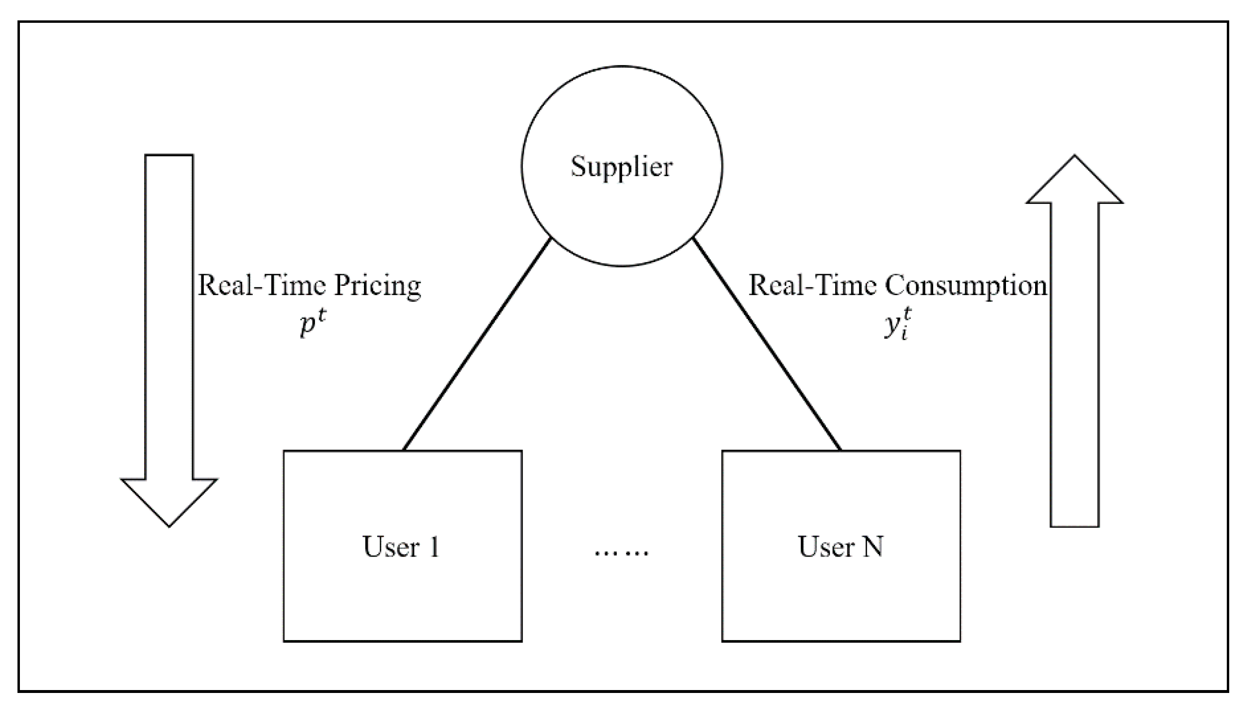
The process covered by these studies is as follows. Under a single price, users’ power demand is concentrated in a specific time period. Concentrated demand requires high power production, and since power production costs are a concave function of production, excessive costs are incurred for suppliers. In addition, in that the initial investment cost of a power generation facility is very large and the construction takes a long time, it is difficult to increase the amount of power generation itself. Therefore, in terms of grid operation, a balanced power demand for each time period is a very important issue. The smart grid and pricing policy solve this problem as follows. First, the supplier decides a price considering the power demand based on the consumers’ information. Then, the consumers respond to the price and adjust their amount of power consumption by time. As a result, the overload and peak-to-average ratio (PAR) are lowered.

In this context, pricing or demand scheduling has become the most important research topic in the field of smart grids. Previous studies can be classified broadly into three categories. The first classification is research dealing with the most basic optimization problem and it is about the demand schedule that maximizes the utility of users. Chen [20] considered energy prices as a given value and found the users’ optimal energy consumptions to maximize their utilities. The second category concerns the maximization of social welfare. Social welfare is a concept that integrates the utility of both sides in the grid system, the supplier and the user, and generally includes the operation profit of the supplier and the welfare or payoff of individual users.

Samadi et al. [21] solved the problem of finding energy prices to maximize social welfare. In this study, they used a distributed algorithm to obtain optimal electricity usage to maximize social welfare, which is defined as the difference in users’ utility and the power supply costs. However, the time preferences of users were randomly designed and the analysis result could not give much information on the impact of user characteristics on social welfare. Deng et al. [20] derived an optimal power usage schedule with a given energy price. This study also introduced a minimum energy demand for users and investigated its impact on the optimal price and consequent social welfare. They proposed a pricing algorithm that does not reduce social welfare while electricity consumption is more evenly distributed. Unlike the above two studies, Chavali et al. [22] derived a usage schedule of various pieces of electronic equipment to minimize user payment. In this study, the user’s cost function was defined as the sum of the electricity bill, the utility obtained from using electricity, and the inconvenience cost felt by delaying the use of electricity. It was shown that the proposed two algorithms have the effect of reducing the cost of users by properly distributing the electricity usage time.

The final classification is studies on the game model between the supplier and the users. In this game, the power supplier wants to maximize their profits and users want to maximize utility. Meng and Zeng [23] and Yu and Hong [24] created real-time pricing models that respond to energy use, which have resulted in real-time pricing that can reduce consumers’ payments and smoothen the imbalance energy supply over time. Meng and Zeng [23] divided electronic products into three categories according to the possibility of delay in use and the need for constant use. In this study, users determine electricity usage strategies to minimize their bills, and the supplier determines real-time prices to maximize profits. Yu and Hong [24] proposed a two-phase model. In the first phase, the electricity supplier minimizes fluctuations in power supply, and in phase II, users maximize the difference between utility and bill. It demonstrated the existence of the Nash equilibrium and the effects of reducing the likelihood of power overloading with the model and increasing user utility through simulation.

Chen et al. [25] conducted a study on a real-time pricing model that reflects the uncertainty in the electricity supply. They designed a more realistic cost function by reflecting the uncertainty. In addition, each user individually maximizes their utility by including user characteristics in the utility function. The effects of real-time pricing were verified by simulation with equilibrium energy prices and energy consumption. Samadi et al. [26] proposed a model that maximizes the overall user utility and minimizes the power supply cost. Through the proposed Vickrey–Clarke–Groves (VCG) mechanism, they confirmed the effect of the smart grid for users to avoid peak times. Qian et al. [27] also proposed a two-stage Stackelberg game model and used an iterative algorithm through which users find their optimal usage and the supplier controls the price. Bu and Yu [28] expanded the existing two-stage game model. They produced more rigorous results by adding two more stages to determine the amount of electricity supplied and the actual electricity usage. Yang et al. [29] compared the results in two situations using a cooperative and non-cooperative game-based approach. Yoon et al. [30] introduced an electric vehicle charging scenario to calculate the optimal electricity usage time, while Yu and Hong [31] defined electronic products as game players and prioritized them to reflect in the utility function for each electronic device. On the other hand, there are also studies that attempted to model the Stackelberg game with multiple electricity suppliers. In a study by Mondal et al. [32], several energy suppliers determine energy prices and minimum energy supplies in Phase 1 and energy users determine the optimal energy schedule in Phase 2. This mechanism resulted in an additional 55% margin for energy suppliers and an approximately 30.79% increase in energy usage for energy users.

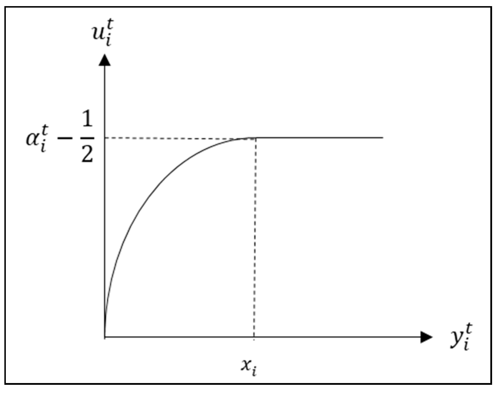
Although a number of studies have been conducted in which game theory has been applied to the smart grid, there is still a gap in the research in terms of time preference. Most studies did not reflect time preference, and studies that considered preference also set preference as a constant value. However, in reality, users have different preferences to use electricity for each time period, and electricity consumption is determined accordingly. Therefore, this study aims to propose a two-stage Stackelberg game model that reflects the time preference of electricity use. Through this model, we want to determine the electricity usage schedule and rate policy that maximizes the utility of users and profits of the supplier. The effectiveness of the proposed real-time pricing (RTP) model is quantitatively verified by comparing it with the results of a system that does not adjust prices in real time. It varies the distribution of consumers’ time preferences and examines the impact on the balance of power demand, power supply cost, usage fee, and social welfare.

This study is novel in directly considering time preference to the utility function and induces a real-time pricing model through a Stackelberg game model. The optimal price and consumption schedule through the Nash equilibrium are derived in the form of a function with respect to the preference, so that the relationship can be directly examined. In addition, this paper attempts to attain a practical contribution in that it examines how the responses of consumers and suppliers differ by performing a simulation by changing time preferences.

2. System Model

We proposed a two-stage Stackelberg game model between an energy supplier and users in this paper. The game consists of one leader (supplier) and a number of followers (users), and each stage of the game corresponds to the optimal consumption scheduling and the optimal pricing problem. The overall structure of the game model is shown in Figure 1. In the first stage, the energy supplier determines the optimal energy price for each time slot to maximize one’s total profit. Following that, energy users determine the optimal energy consumption in each time slot.

2.1. Real-Time Pricing Model

A real-time pricing model between an energy supplier and multiple users is proposed as a two-stage Stackelberg game model in this paper. In the first stage, the energy supplier, who acts as a leader, decides the optimal real-time price for each time slot which maximizes profit by supplying energy. Then, in the second stage, each user decides the optimal energy consumption which maximize ones’ payoff reflecting users’ time preference. The notations used in this paper are as listed in

Table 1. Notations.

Parameter	Description
$p^t$	Energy price at time $t$
$x_i$	Maximum daily requirement of user $i$
${\alpha }_i^t$	Time preference (weight) for user $i$ at time $t$
$T$	Number of time slots
$N$	Number of users
$y_i^t$	Actual consumption of user $i$ at time $t$
$y$	Matrix of users’ energy consumption schedule
$p$	Vector of supplier’s energy supplement schedule
$Y^t$	Total amount of energy consumption at time $t$
$\mathsf{\Pi }$	Profit obtained by the energy supplier during time period $[1,T]$
$C^t$	Cost function of energy generation
$d_i^t$	Coefficients of cost function ($i=1,2,3$)
$K$	Production capacity for each time slot
$u_i^t$	Utility of user $i$ at time $t$
$W_i$	Payoff of user $i$ for using energy

.

2.1.1. Supplier-Side Model

In the first stage, the supplier determines the price of electricity to maximize profits. A supplier’s profit is the difference between the sum of electricity bills paid by users and the cost to generate electricity. The production cost is calculated for each time period, and the cost function ($C(Y^t)$) is defined as a function of the total amount of electricity consumption for the time period ($Y^t={\displaystyle \sum _{i=1}^N{y}_i^t}$), and should have the following properties.

Property 1.

Energy generation cost($C(Y^t)$) is increasing as$Y^t$, i.e.,$\frac{\partial C(Y^t)}{\partial Y^t}>0, \forall t\in [1,T]$.

Property 2.

The cost function is strictly convex. I.e.,$\frac{{\partial }^{2}C(Y^t)}{\partial {(Y^t)}^2}>0, \forall t\in [1,T]$.

Property 3.

There exists a differentiable, convex, non-decreasing function$p_k(q)\ge 0$over$q\ge 0$for each$k\in \kappa$with$p_k(q)\ge 0$and$p_k(q)\to \infty$as$q\to \infty$, such that for$q\ge 0$,$C_k(q)={\displaystyle {\int }_0^q{p}_k(z)dz}$.

Following the cost function proposed in many previous studies, we adopted the quadratic form for the energy generation function, $C^t(Y^t)=d_1^t{(Y^t)}^2+d_2^t{Y}^t+d_3^t, (d_1^t>0, d_2^t\ge 0, d_3^t\ge 0)$.

Since the revenue can be expressed as the sum of products of energy price and consumption at each time slot ($p^t\left({\displaystyle \sum _{i=1}^N{y}_i^t}\right)$), the supplier’s profit at time $t$ is defined as $p^t\left({\displaystyle \sum _{i=1}^N{y}_i^t}\right)-C^t\left({\displaystyle \sum _{i=1}^N{y}_i^t}\right)$. Thus, the decision problem for supplier is as follows.

$$\begin{array}{l}\max \mathsf{\Pi }(p)={\displaystyle \sum _{t=1}^T{p}^t\left({\displaystyle \sum _{i=1}^N{y}_i^t}\right)}-{\displaystyle \sum _{t=1}^T{C}^t\left({\displaystyle \sum _{i=1}^N{y}_i^t}\right)}\\ s.t.{\displaystyle \sum _{i=1}^N{y}_i^t}\le K, \forall i\in [1,N]\end{array}$$

(1)

2.1.2. User-Side Model

Given the optimized prices decided by energy supplier in the first stage, users decide their energy consumption schedule in the second stage. We define the payoff of the users as the difference between utility and payment for energy usage. The user utility function is defined over the amount of used energy for a given time slot and includes time preference property. Generally, a utility function satisfies following Properties 4–6.

Property 4.

The utility function is non-decreasing with respect to the energy consumption($y_i^t$). I.e.,$\frac{\partial u_i^t}{\partial y_i^t}\ge 0, \forall i\in [1,N], \forall t\in [1,T]$.

Property 5.

The utility function is concave. I.e.,$\frac{{\partial }^2{u}_i^t}{\partial y_i^{t^2}}\le 0, \forall i\in [1,N], \forall t\in [1,T]$.

Property 6.

When energy consumption is zero, the utility is zero, i.e.,$u_i^t=0$, if$y_i^t=0,\forall i\in [1,N]$.

In this study, time preference was reflected in the utility function. Time preference is included in the form of a coefficient value, and the value is designed to increase as the power consumption of the time is preferred. The coefficient ${\alpha }_i^t$ represents the time preference of user $i$ to use electricity in the time interval $t$. A bigger value of ${\alpha }_i^t$ means the user wants to use more electricity.

Property 7.

The utility function increases with respect to the time preference parameter(${\alpha }_i^t$), i.e.,$\frac{\partial u_i^t}{\partial {\alpha }_i^t}>0, \forall i\in [1,N], \forall t\in [1,T]$.

In addition, the utility should stop increasing when the consumption exceeds one’s maximum daily demand. With satisfying these properties, we will define the utility function as following Equation (2), which is a modified quadratic utility function.

$$u_i^t(y_i^t, {\alpha }_i^t)=\{\begin{array}{c}-\frac{1}{2}{\left(\frac{y_i^t}{x_i}\right)}^2+{\alpha }_i^t\left(\frac{y_i^t}{x_i}\right), y_i^t\le x_i\\ {\alpha }_i^t-\frac{1}{2}, y_i^t>x_i\end{array}$$

(2)

The quadratic utility function is the most common form of function that describes a consumer’s utility. We have modified the default form to incorporate the maximum daily demand. In the case of the quadratic utility function, a range of input values that decrease utility may occur. To solve this problem, we assume a form where the utility no longer increases before the peak of the quadratic function. The maximum point will be in a situation that is difficult to reach in reality, so it is advisable to set it to an extreme limit. Note that in a real power network, the user’s maximum utility can be regarded as the case of using the maximum demand. Therefore, we assume that the maximum daily electricity demand desired by the user is the limit input value of the utility function that is used at a specific time period.

To satisfy the properties above, the time preference coefficient is defined as ${\alpha }_i^t\ge 1$. The utility function is shown in Figure 2.

The proposed function satisfies the properties above as follows.

Proof of Property 4.

$\frac{\partial u_i^t}{\partial y_i^t}=\frac{1}{x_i}\left(-\frac{y_i^t}{x_i}+{\alpha }_i^t\right)>0$ for $y_i^t<x_i$. It is obvious for ${\alpha }_i^t\ge 1$. □

Proof for Property 5.

$\frac{{\partial }^2{u}_i^t}{\partial y_i^{t^2}}=-\frac{1}{{\left(x_i\right)}^2}<0$. □

Proof for Property 6.

$u_i^t\left(y_i^t=0\right)=-\frac{1}{2}{\left(\frac{0}{x_i}\right)}^2+{\alpha }_i^t\frac{0}{x_i}=0$. □

Proof for Property 7.

$\frac{\partial u_i^t}{\partial {\alpha }_i^t}=\frac{y_i^t}{x_i}>0$. □

Now, the payoff of the energy user $i$ at time $t$ is given by $u_i^t(y_i^t)-p^t{y}_i^t$, and the decision model for the user $i$ is defined as Equation (3).

$$\begin{array}{l}\max W_i(y_i)={\displaystyle \sum _{t=1}^T\left[-\frac{1}{2}{\left(\frac{y_i^t}{x_i}\right)}^2+{\alpha }_i^t\frac{y_i^t}{x_i}\right]}-{\displaystyle \sum _{t=1}^T{p}^t{y}_i^t}\\ s.t.\hspace{1em}{\displaystyle \sum _{t=1}^T{y}_i^t\le x_i, \forall i\in [1,N]}\end{array}$$

(3)

2.2. Non-Real-Time Pricing Model

To verify the effect of real-time pricing in a smart grid, we also made a non-real-time pricing model. The non-real-time pricing model is almost the same as the real-time pricing model, except that the energy price is constant over time. Thus, the decision models on the supplier’s side and users’ side are defined as follows.

$$\begin{array}{l}\max \mathrm{\Pi }(p)=p{\displaystyle \sum _{t=1}^T\left({\displaystyle \sum _{i=1}^N{y}_i^t}\right)}-{\displaystyle \sum _{t=1}^T{C}^t\left({\displaystyle \sum _{i=1}^N{y}_i^t}\right)}\\ s.t.{\displaystyle \sum _{i=1}^N{y}_i^t}\le K, \forall i\in [1,N]\end{array}$$

(4)

$$\begin{array}{l}\max W_i(y_i)={\displaystyle \sum _{t=1}^T\left[-\frac{1}{2}{\left(\frac{y_i^t}{x_i}\right)}^2+{\alpha }_i^t\frac{y_i^t}{x_i}\right]}-p{\displaystyle \sum _{t=1}^T{y}_i^t}\\ s.t.\hspace{1em}{\displaystyle \sum _{t=1}^T{y}_i^t\le x_i, \forall i\in [1,N]}\end{array}$$

(5)

3. Equilibrium

3.1. Equilibrium of Real-Time-Pricing Model

The method of Karush–Kuhn–Tucker (KKT) conditions was employed to solve the optimization problems defined in the system model part. The equilibrium of the real-time pricing model is obtained as Proposition 1. The detailed proof is described in Appendix A.

Proposition 1.

(Equilibrium of real-time pricing model).

A. 

If${\displaystyle {\sum }_{t=1}^T\left({\alpha }_i^t-p^t{x}_i\right)\le 1}$, and$\frac{{\alpha }_i^t}{x_i}\ge p^t$:

i. 

If${\displaystyle {\sum }_{i=1}^N{y}_i^t}<K$, the optimal energy price and consumption are given by

$$p^{t*}=\frac{{\displaystyle \sum _{i=1}^N\left({\alpha }_i^t{x}_i\right)+d_2^t{\displaystyle \sum _{i=1}^N{\left(x_i\right)}^2}}}{2{\displaystyle \sum _{i=1}^N{\left(x_i\right)}^2}}, y_i^{t*}={\alpha }_i^t{x}_i-\frac{{\displaystyle \sum _{i=1}^N\left({\alpha }_i^t{x}_i\right)+d_2^t{\displaystyle \sum _{i=1}^N{\left(x_i\right)}^2}}}{2{\displaystyle \sum _{i=1}^N{\left(x_i\right)}^2}}{\left(x_i\right)}^2$$

ii. 

If${\displaystyle {\sum }_{i=1}^N{y}_i^t}=K$, the optimal energy price and consumption are given by

$$p^{t*}=\frac{{\displaystyle \sum _{i=1}^N\left({\alpha }_i^t{x}_i\right)-K}}{2{\displaystyle \sum _{i=1}^N{\left(x_i\right)}^2}}, y_i^{t*}={\alpha }_i^t{x}_i-\frac{{\displaystyle \sum _{i=1}^N\left({\alpha }_i^t{x}_i\right)-K}}{2{\displaystyle \sum _{i=1}^N{\left(x_i\right)}^2}}{\left(x_i\right)}^2$$

B. 

If${\displaystyle {\sum }_{t=1}^T\left({\alpha }_i^t-p^t{x}_i\right)>1}$, and$\frac{{\alpha }_i^t}{x_i}\ge p^t$, the optimal energy price and consumption are given by${\displaystyle {\sum }_{t=1}^T{y}_i^{t*}}=x_i$,$p^{t*}\to +\infty$

C. 

If$\frac{{\alpha }_i^t}{x_i}<p^t$, the optimal energy price and consumption is given by$p^{t*}=0$, and$y^{t*}=0$.

The parts of B and C are boundary solutions and have little intuition, so we only consider the solution given in part A.

3.2. Comparative Statics

Based on the equilibrium obtained above, we performed comparative statics to investigate the relationships between the variables. The results are given by Propositions 2–5.

Proposition 2.

Energy consumption for the user$i$at$t$increases as time preference (${\alpha }_i^t$) increases, i.e.,$\frac{\partial y_i^{t*}}{\partial {\alpha }_i^t}>0$.

Proof. 

$\frac{\partial y_i^{t*}}{\partial {\alpha }_i^t}=x_i-\frac{{\left(x_i\right)}^3}{2{\displaystyle \sum _{i=1}^N{\left(x_i\right)}^2}}=x_i\left(1-\frac{{\left(x_i\right)}^2}{2{\displaystyle \sum _{i=1}^N{\left(x_i\right)}^2}}\right)>0$. □

Proposition 3.

A higher time preference gives a higher energy price, i.e.,$\frac{\partial p^{t*}}{\partial {\displaystyle {\sum }_{i=1}^N{\alpha }_i^t}}>0$.

Proof. 

$\frac{\partial p^{t*}}{\partial {\displaystyle {\sum }_{i=1}^N{\alpha }_i^t}}=\frac{x_i}{2{\displaystyle \sum _{i=1}^N{\left(x_i\right)}^2}}>0$. □

Proposition 4.

Energy consumption decreases as the price goes up, i.e.,$\frac{\partial y_i^{t*}}{\partial p^t}<0$.

Proof. 

$\frac{\partial y_i^{t*}}{\partial p^t}=-{\left(x_i\right)}^2<0$. □

Proposition 5.

Energy price does not decrease as first-order coefficient of cost function($d_2^t$) increases, i.e.,$\frac{\partial p^{t*}}{\partial d_2^t}\ge 0$.

Proof. 

$\frac{\partial p^{t*}}{\partial d_2^t}=\frac{{\displaystyle \sum _{i=1}^N{\left(x_i\right)}^2}}{2{\displaystyle \sum _{i=1}^N{\left(x_i\right)}^2}}=\frac{1}{2}>0$. □

The results of the comparative statics are intuitive. Thus, we will perform a numerical analysis based on the equilibrium obtained above.

3.3. Equilibrium of Non-Real-Time Pricing Model

Similarly, the method of KKT conditions was employed to solve the non-real-time pricing optimization problems defined in the system model part. The equilibrium of non-real-time-pricing model is obtained as Proposition 2.

Proposition 6.

(Equilibrium of non-real-time pricing model).

A. 

If${\displaystyle {\sum }_{t=1}^T\left({\alpha }_i^t-p{x}_i\right)\le 1}$, and$\frac{{\alpha }_i^t}{x_i}\ge p$:

i. 

If${\displaystyle {\sum }_{i=1}^N{y}_i^t}<K$, the optimal energy price and consumption are given by

$$p^{*}=\frac{{\displaystyle \sum _{t=1}^T{\displaystyle \sum _{i=1}^N\left({\alpha }_i^t{x}_i\right)}}+{\displaystyle \sum _{t=1}^T{\displaystyle \sum _{i=1}^N{d}_2^t{\left(x_i\right)}^2}}}{2T{\displaystyle \sum _{i=1}^N{\left(x_i\right)}^2}}, y_i^{t*}={\alpha }_i^t{x}_i-\frac{{\displaystyle \sum _{t=1}^T{\displaystyle \sum _{i=1}^N\left({\alpha }_i^t{x}_i\right)}}+{\displaystyle \sum _{t=1}^T{\displaystyle \sum _{i=1}^N{d}_2^t{\left(x_i\right)}^2}}}{2T{\displaystyle \sum _{i=1}^N{\left(x_i\right)}^2}}{\left(x_i\right)}^2$$

ii. 

If${\displaystyle {\sum }_{i=1}^N{y}_i^t}=K$, the optimal energy price and consumption are given by

$$p^{*}=\frac{{\displaystyle \sum _{i=1}^N\left({\alpha }_i^t{x}_i\right)-K}}{{\displaystyle \sum _{i=1}^N{\left(x_i\right)}^2}}, y_i^{t*}={\alpha }_i^t{x}_i-\frac{{\displaystyle \sum _{i=1}^N\left({\alpha }_i^t{x}_i\right)-K}}{{\displaystyle \sum _{i=1}^N{\left(x_i\right)}^2}}{\left(x_i\right)}^2$$

B. 

If${\displaystyle {\sum }_{t=1}^T\left({\alpha }_i^t-p{x}_i\right)>1}$, and$\frac{{\alpha }_i^t}{x_i}\ge p$, the optimal energy price and consumption are given by${\displaystyle {\sum }_{t=1}^T{y}_i^{t*}}=x_i$,$p^{*}\to +\infty$

C. 

If$\frac{{\alpha }_i^t}{x_i}<p$, the optimal energy price and consumption are given by$p^{*}=0$, and$y^{t*}=0$.

Furthermore, the parts of B and C are boundary solutions and have little intuition, so we only consider the solution given in part A.

4. Numerical Analysis

In this section, a simulation experiment is demonstrated to verify the game model and its equilibrium, proposed above. The target smart grid is designed with one supplier and 10 individual users with different time preferences. Two time slots, non-peak and peak, are defined over the experiment horizon of one day. The demonstration has two purposes. First, it is developed to show the effect of real-time pricing (RTP) over non-real-time pricing (NRTP) by comparing the results from each setting. Second, the impact of the changes in time preferences on the grid is qualitatively investigated.

For convenience, time preferences to non-peak time are fixed as 1, while the peak time preferences increase from 1.2 to 1.6 as shown in Figure 3. Consequently, in total, 20 sets of experiment settings with different peak time preferences were prepared.

To give a little reality to the experiment, 100 Monte Carlo simulations were performed for each setting. For each repetition, the user’s daily maximum power requirement and time preference values for each time period were randomly generated. In the case of the maximum daily requirement, an error of 5% was applied, and an error of 3% was applied to the preference values. As a result, 100 repeated experiments were performed for each of the 20 settings, and the averaged values of the repeated results were summarized as the result values.

4.1. User-Side Result

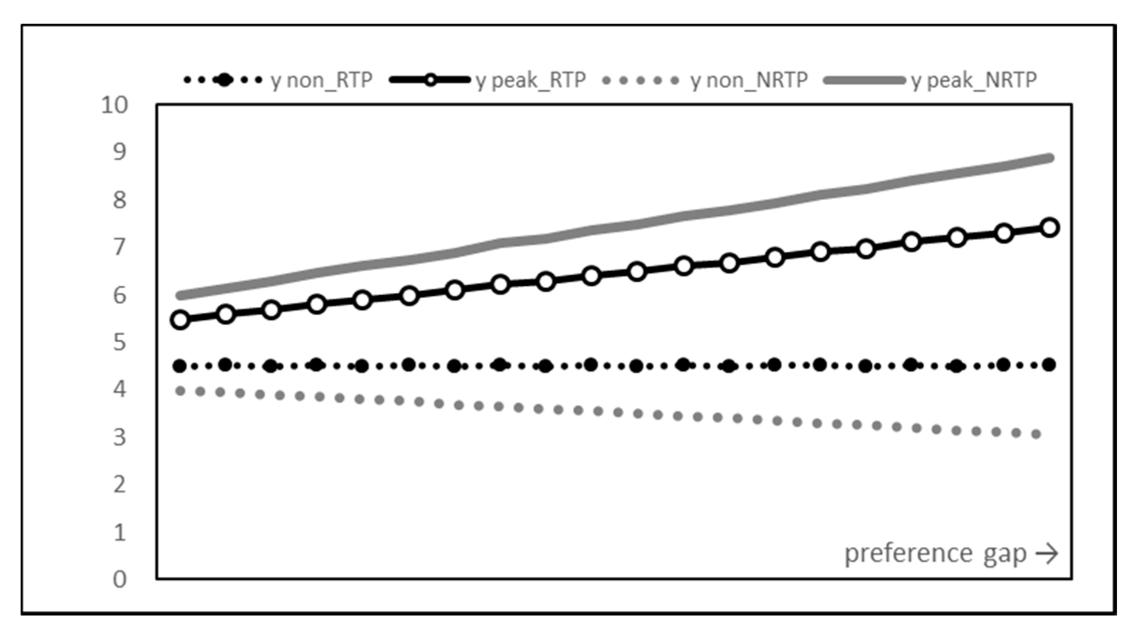
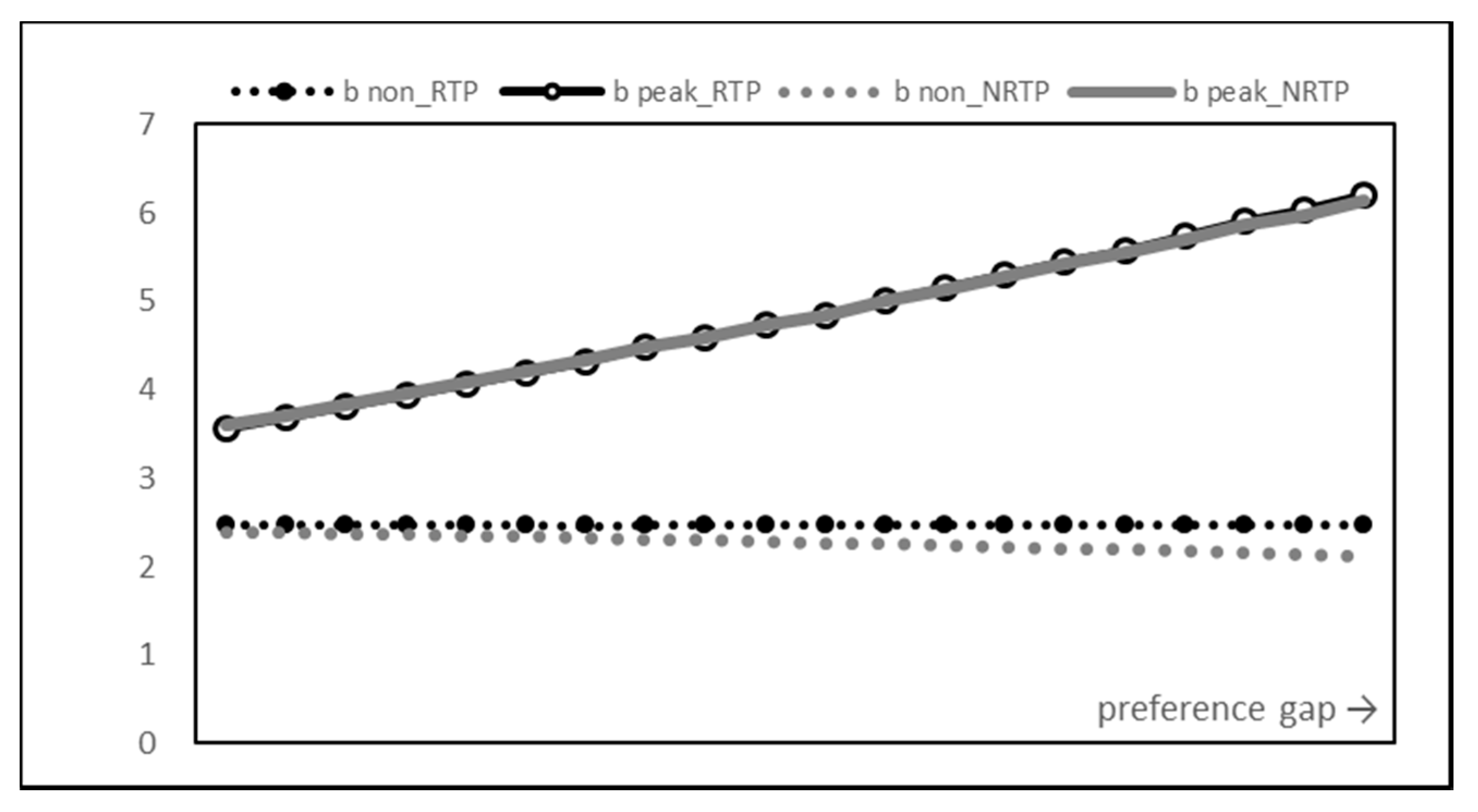
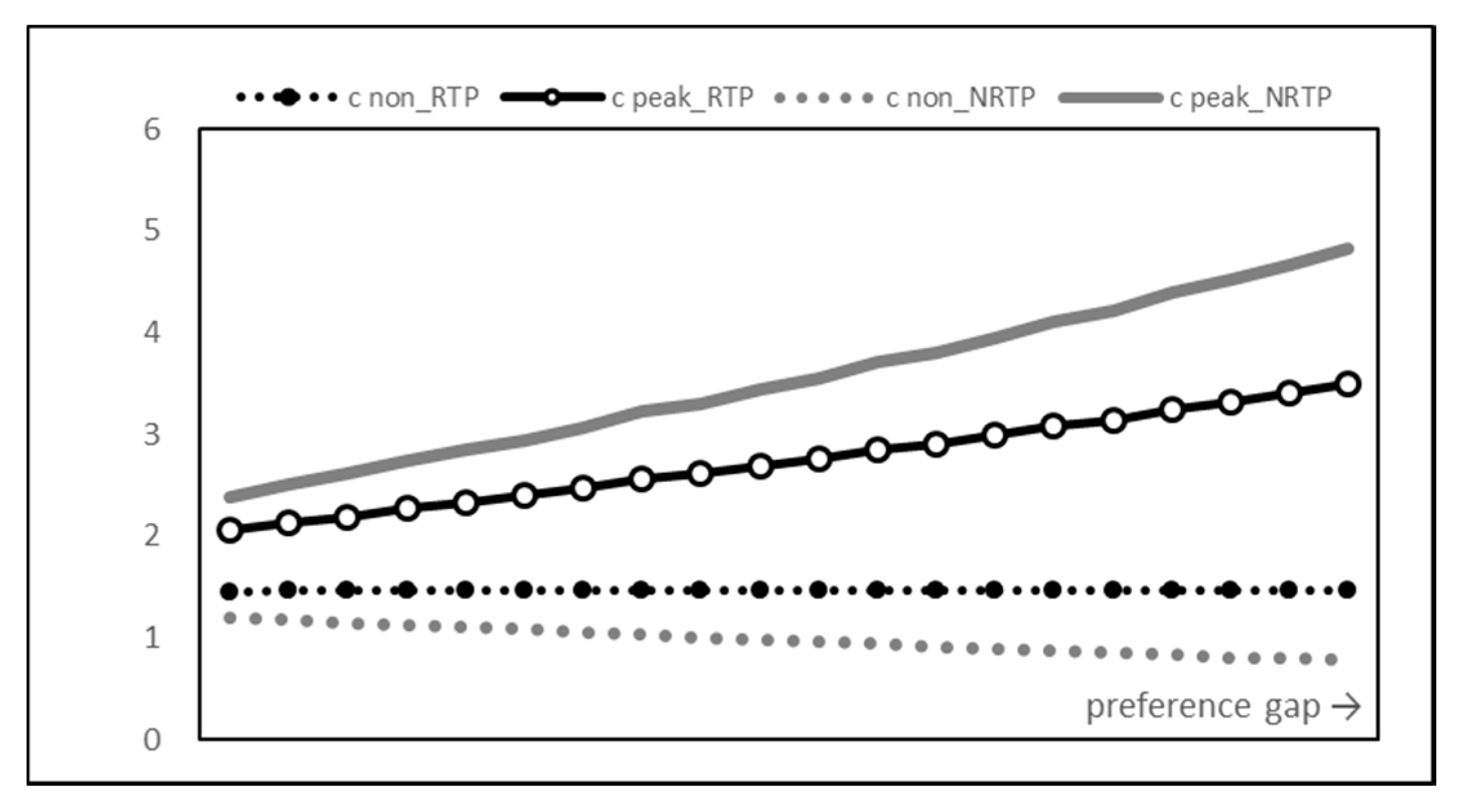
First of all, we looked at the change in the power consumption pattern of users. Figure 4 shows how RTP and NRTP affect users as the preference gap, the difference (${\alpha }_{peak}-{\alpha }_{nonpeak}$) between the peak time and the non-peak time preference, increases.

Lines with points are the results of RTP, and lines without points are the results of NRTP. In addition, the solid line represents the peak time and the dotted line represents the non-peak time. As expected, RTP closes the power usage gap between peak and non-peak times. This is in contrast to the large increase in the power usage gap in the NRTP results.

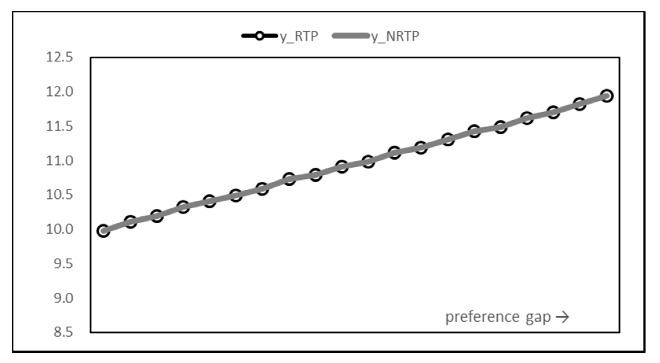
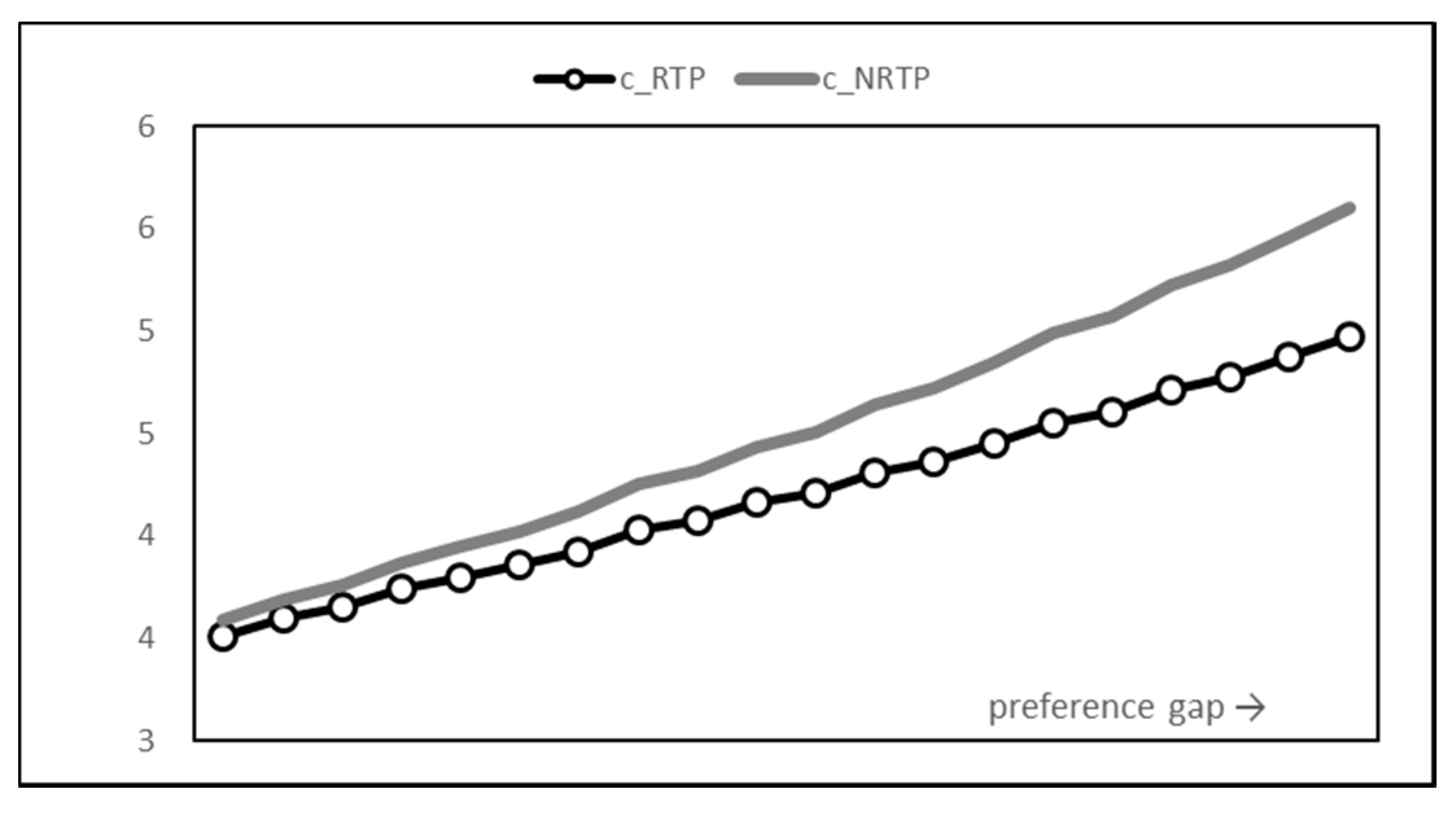
However, the total energy consumption in Figure 5 shows that there is little difference in the results of the two methods. In other words, the introduction of RTP can be understood as shifting the power consumption period rather than reducing the power consumption. Another fact that can be seen from the graph is that the total power usage is steadily increasing. It seems that the usage that maximizes payoff also increases as the utility increases due to the increase in time preference.

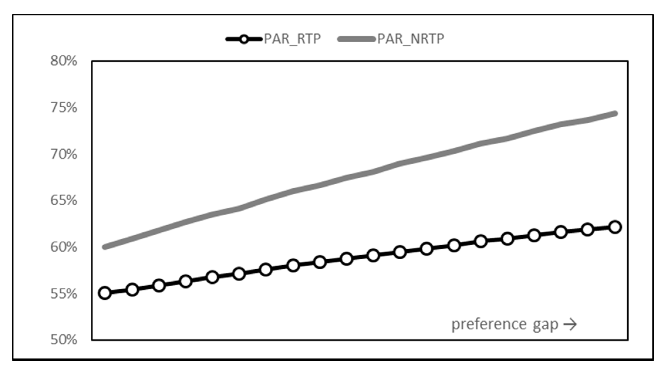
Peak-to-average ratio (PAR), which is defined as the ratio of energy consumption at peak time and average energy consumption, is a measure of the load of the energy generator. A lower PAR value means that the energy consumptions are distributed more evenly. Thus, the lower the PAR value is, the less overload cases will occur.

Figure 6 shows the PAR values. Consistent with the consumption results, the PAR value of RTP was significantly lower than that of NRTP. When the time preference gap was at the maximum, the results of NRTP showed that more than 74% of the power consumption was concentrated on the peak time, but when RTP was introduced, it was suppressed to 62%. This means that even when the peak time preference of users becomes intensified, the risk of overload can be suppressed to a very low level through the introduction of a smart grid and RTP.

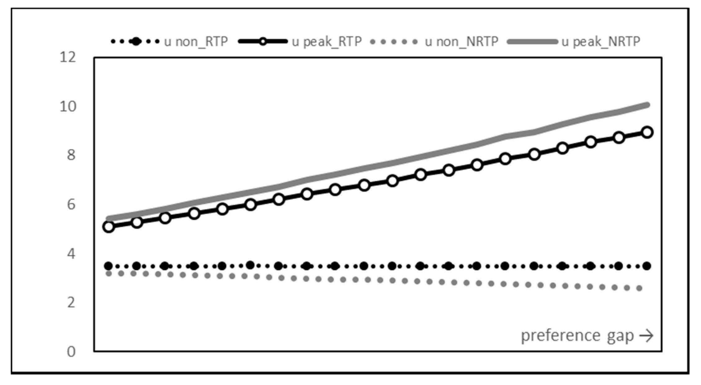
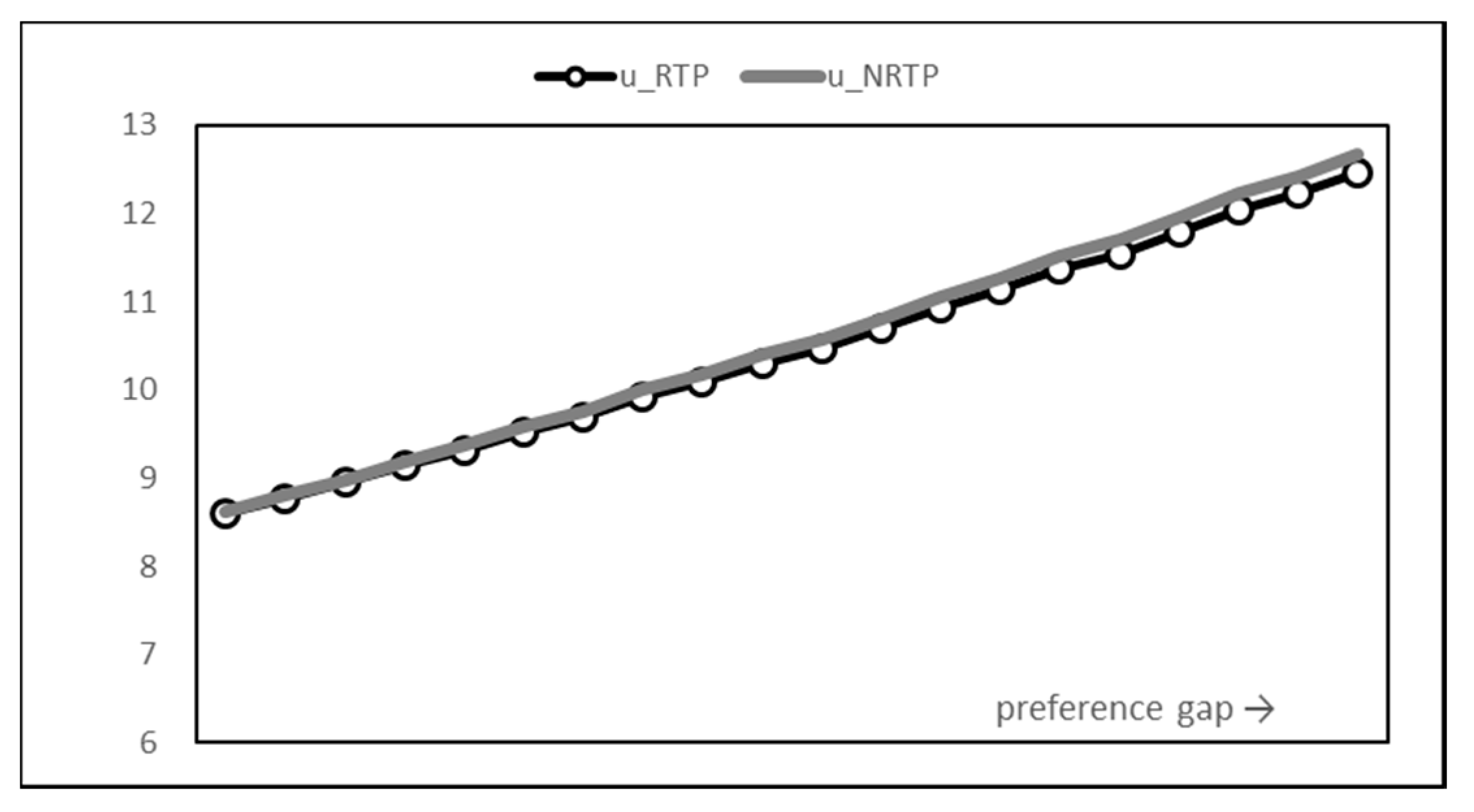
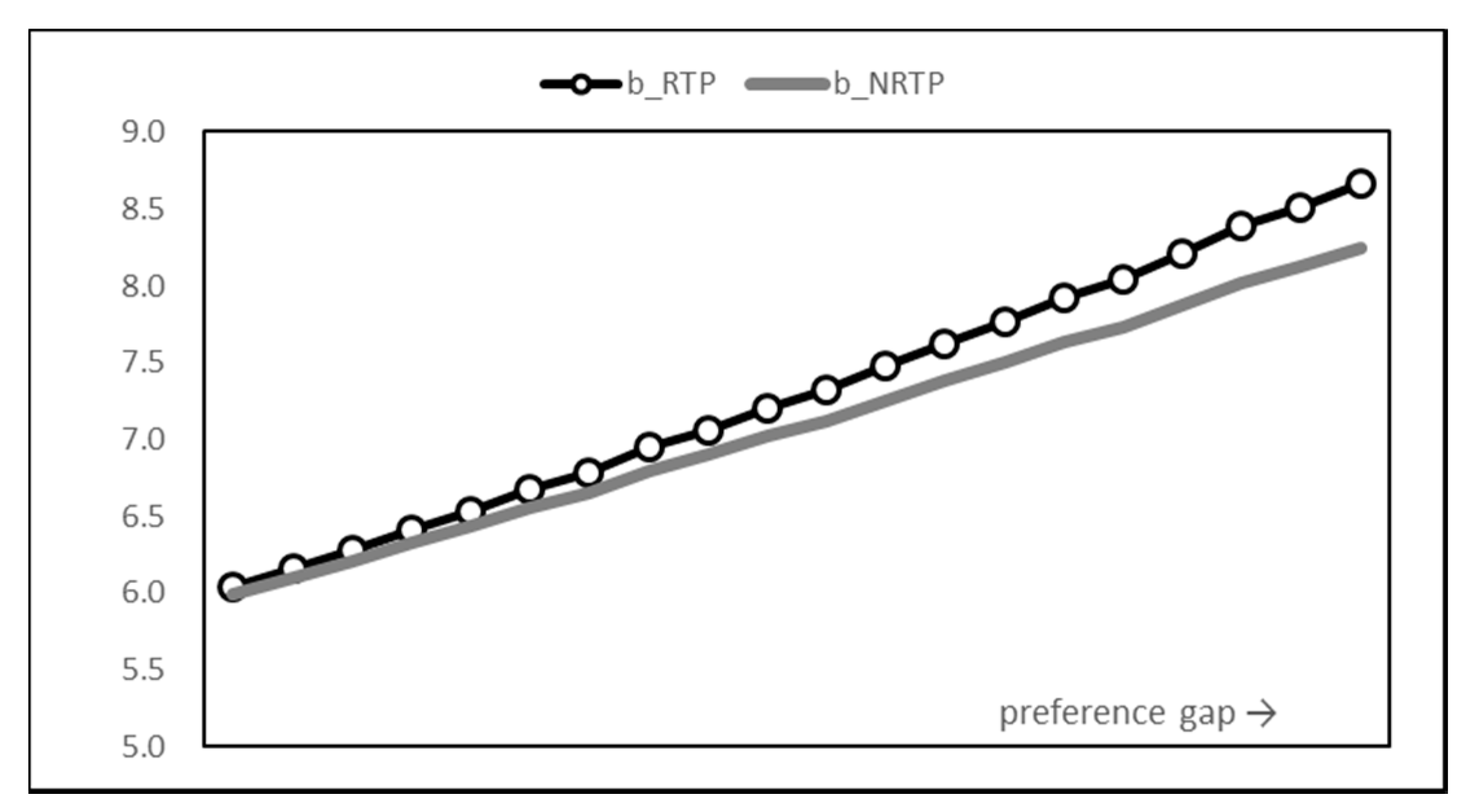
Figure 7 and Figure 8 show the change in utility. A pattern similar to the result of previous consumption is found. As the time preference coefficient value of the peak time increases, the overall utility value increases steadily. The introduction of RTP rarely changes the overall utility but rather reduces it very little. The introduction of RTP leads to a decrease in the utility of the peak time and an increase in the utility of the non-peak time, but the balancing effect of the utility is small compared to that of consumption.

Figure 9 and Figure 10 are graphs of bill payments. Though the introduction of RTP reduced peak time consumption, the bill payment was almost the same as that with NRTP because the supplier raised the price. On the other hand, the RTP is higher for the non-peak time bill. This is because non-peak usage increased significantly in the RTP results. As a result, the total bill payment for all consumers increases slightly in RTP.

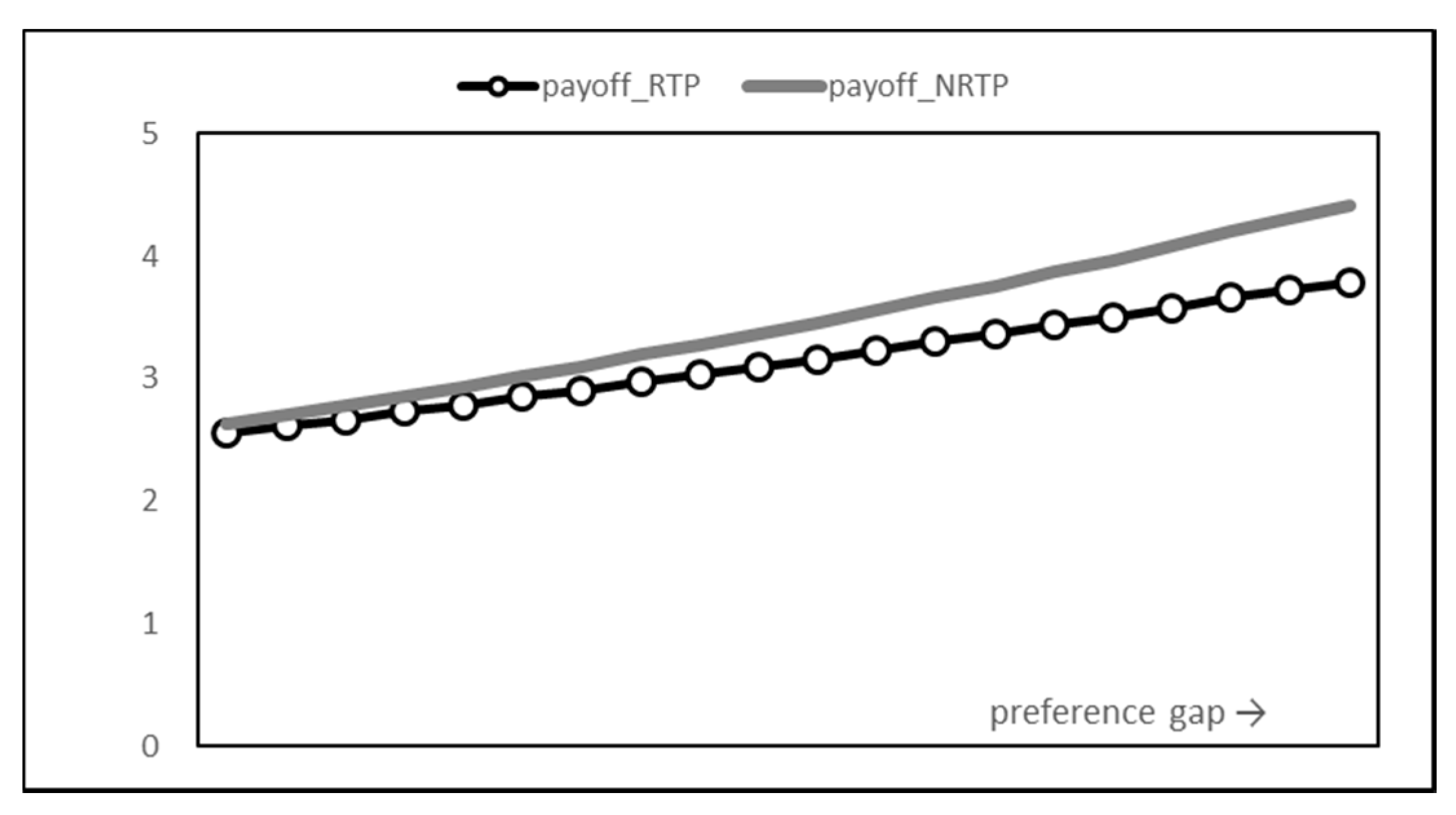
Figure 11 shows the final payoff of the consumer. According to the results of the utility and billing costs discussed above, RTP shows a relatively low payoff compared to NRTP. Overall, the introduction of RTP induces users to shift energy consumption from peak time to non-peak time. As a result, there is no significant change in overall utility, but payoff slightly decreases due to an increase in payment cost. This result is thought to be due to a large increase in the peak time price of the supplier due to the introduction of RTP. Analysis of the supplier’s results in the following section supports this interpretation.

4.2. Supplier-Side Result

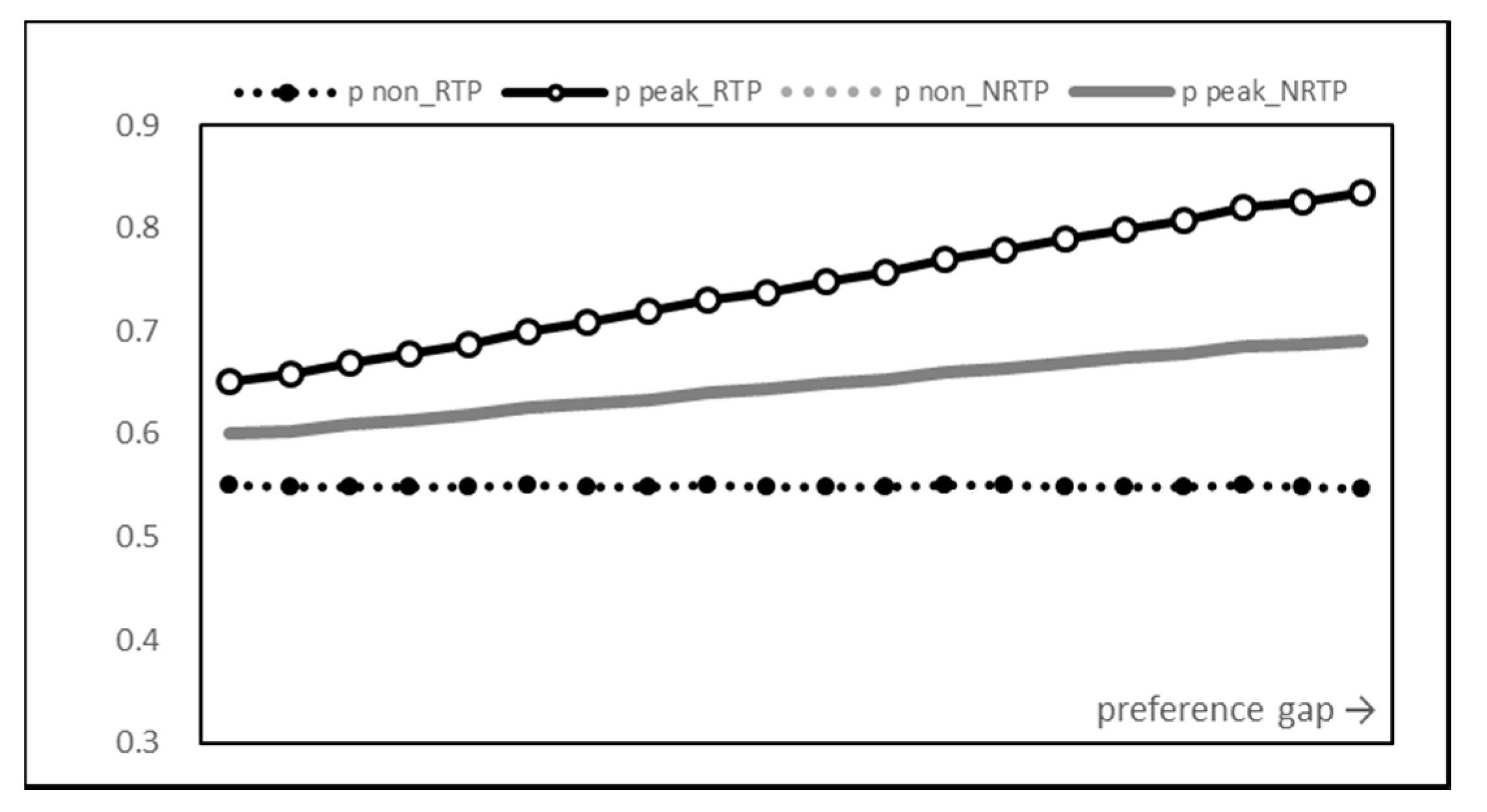
The supplier’s response to changes in time preference is price adjustment. Figure 12 shows the pattern in which RTP differentiates prices by time slots. As the time preference gap increases, the single price under NRTP increases steadily. The average price from RTP also increases steadily, but the non-peak time price hardly changes. Instead, the peak time price of RTP increases significantly, inducing consumers to reduce peak time consumption. In the last setting experiment, RTP set a peak time price more than 50% higher than the non-peak time price.

Figure 13 and Figure 14 show the supplier’s electricity production costs determined according to the energy consumption in Figure 4. Same as the consumption pattern, it can be seen that the difference between the peak time and non-peak time production cost of RTP is much smaller than that of NRTP. However, the total sum result is different from consumption. The total amount of energy consumption was the same for both RTP and NRTP, but there is a difference in power generation cost. Figure 14 demonstrates that the introduction of RTP has the effect of reducing power production costs. This is because the cost function is quadratic, so even if the sum is constant, the cost can be reduced through balanced distribution.

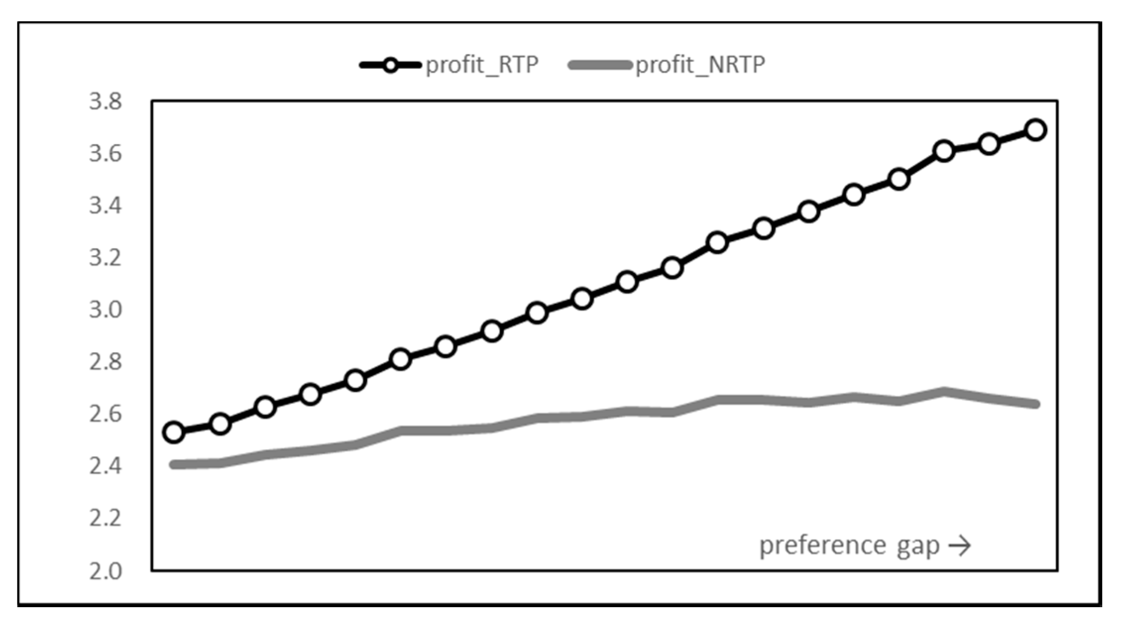
The electricity bill paid by users becomes the supplier’s revenue. Therefore, the profit of the supplier can be obtained by deducting the total consumer bill in Figure 10 and the production cost in Figure 14. As previously shown, RTP increases the user’s electricity bill and lowers the supplier’s electricity production costs. As a result, the profit gap depicted in Figure 15 occurs. When the time preference gap increases, NRTP hardly changes the supplier’s profit. In other words, the production cost increases as the income from electricity usage increases. On the other hand, RTP lowers the increase in production cost compared to NRTP and improves the final profit by further increasing consumption fee income. In fact, comparing the results of the first and last settings, the profit from NRTP increased by only 10%, but the profit from RTP increased by 46%. In the final setting, the gap between the two profits is 40% based on NRTP.

4.3. Social Welfare

The direct effect that can be expected from the introduction of RTP is the alleviation of overload caused by concentrated consumption in a specific time period. As discussed above, the proposed methodology greatly improved the PAR. Through this, social costs, such as additional power infrastructure construction costs, can be avoided or deferred.

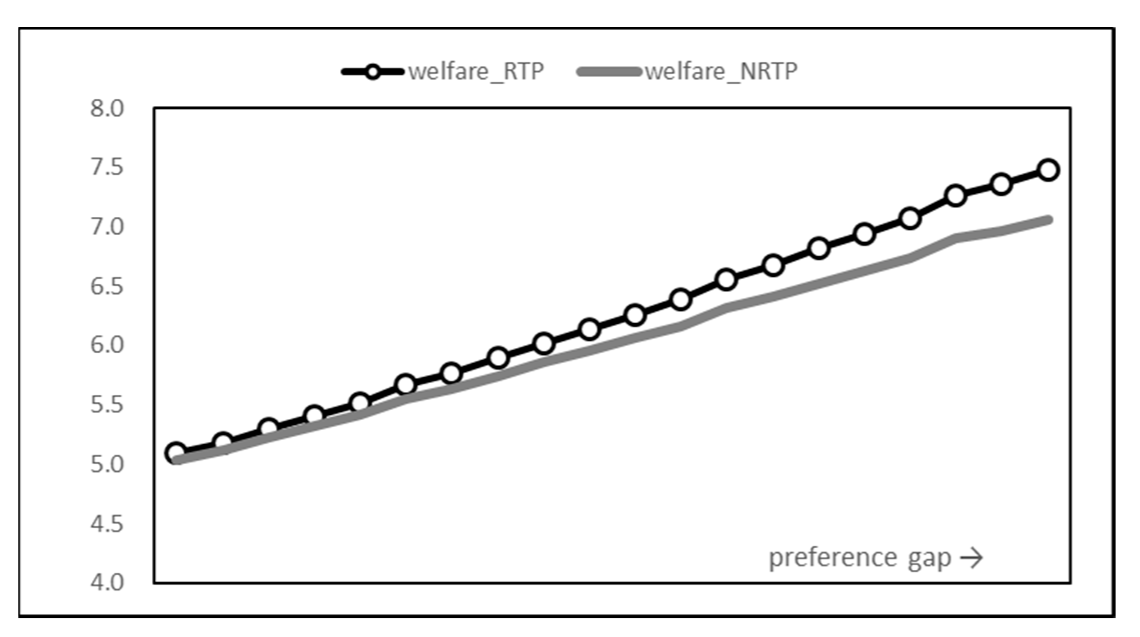
Another effect confirmed through the simulation is the improvement of the welfare of the system as a whole. Social welfare is defined as the sum of supplier profit and consumer payoff and is a measure that considers all participants in the entire smart grid network.

Figure 16 shows the trend of social welfare changes. As the difference in time preference between the two time zones increases, the overall welfare also increases. However, this increase is basically due to an increase in utility resulting from an increase in the peak time preference coefficient and an increase in the supplier’s income with the higher price. RTP shows clear welfare improvement compared to NRTP. It can be seen that as the disparity between users’ preferences by time zone increases, the introduction of RTP significantly improves the profits of suppliers particularly, thereby improving overall social welfare. In other words, RTP led to a greater profit increase than the decrease in consumer payoff. From the first setting, RTP consistently produced a higher welfare value than NRTP, and the last setting showed a gap of 6%.

It is clear that RTP benefits the entire power system by improving PAR and welfare. However, as can be seen in the experiment, the benefits of users and consumers may vary according to the relative size of the parameter value. Taking the results of our experiment as an example, the overall social welfare improved, but the payoff of consumers did not. Therefore, it is believed that efforts to evenly distribute the benefits of the entire system are necessary.

5. Conclusions

The introduction of the smart grid has the effect of distributing the power demand concentrated in a specific hour to other time slots. This imbalanced demand is essentially due to users’ preferences across time.

In this study, we proposed a real-time pricing method for a smart grid through a two-stage Stackelberg game model based on a utility function that reflects the user’s time preference. In the first stage, the supplier determines a price that maximizes profits, and in the next stage, users decide on electricity usage according to the given price. The Nash equilibrium and comparative analysis of the proposed model explain the relationship between time preference, price, and usage. In addition, the changes according to the distribution of time preferences were demonstrated through a Monte Carlo simulation experiment. The results confirmed that the proposed RTP method has the effect of lowering PAR and increasing overall social welfare.

This study is meaningful in that it presents a pricing model that considers both the strategies of users and suppliers and is novel in reflecting users’ time preferences. The proposed model would help to reduce the need for additional power generation facilities by lowering the maximum power generation requirement through efficient operation of a smart grid.

However, the parameters used in the experiment are arbitrarily set, so there is a limit of reality. To overcome this, it is necessary to use empirical data in future studies. In other words, it will be a more valuable study if actual consumers’ power consumption and suppliers’ price trends are used to analyze consumers’ time preference and price sensitivity and apply it to the experiment.

References

1. Arroyo, M.F.R.; Miguel, L.J. The Role of Renewable Energies for the Sustainable Energy Governance and Environmental Policies for the Mitigation of Climate Change in Ecuador. Energies 2020, 13, 3883. [Google Scholar] [CrossRef]
2. Karlsdottir, M.R.; Heinonen, J.; Palsson, H.; Palsson, O.P. High-Temperature Geothermal Utilization in the Context of European Energy Policy—Implications and Limitations. Energies 2020, 13, 3187. [Google Scholar] [CrossRef]
3. Andoni, M.; Robu, V.; Früh, W.G.; Flynn, D. Game-theoretic modeling of curtailment rules and network investments with distributed generation. Appl. Energy 2017, 201, 174–187. [Google Scholar] [CrossRef] [Green Version]
4. Bronski, P.; Creyts, J.; Crowdis, M.; Doig, S.; Glassmire, J.; Guccione, L.; Lilienthal, P.; Mandel, J.; Rader, B.; Seif, D. The economics of load defection: How grid-connected solar-plus-battery systems will compete with traditional electric service–why it matters, and possible paths forward. Rocky Mountain Institute. 2015. Available online: https://rmi.org/insight/the-economics-of-load-defection-how-grid-connected-solar-plus-battery-systems-will-compete-with-traditional-electric-service-why-it-matters-and-possible-paths-forward-executive-summary/ (accessed on 10 October 2020).
5. Asimakopoulou, G.E.; Dimeas, A.L.; Hatziargyriou, N.D. Leader-follower strategies for energy management of multi-microgrids. IEEE Trans. Smart Grid 2013, 4, 1909–1916. [Google Scholar] [CrossRef]
6. Kathan, D.; Daly, C.; Eversole, E.; Farinella, M.; Gadani, J.; Irwin, R.; Lankford, C.; Pan, A.; Switzer, C.; Wright, D. National action plan on demand response. The Federal Energy Regulatorycommission Staff. 2010. Available online: https://www.energy.gov/sites/prod/files/oeprod/DocumentsandMedia/FERC_NAPDR_-_final.pdf (accessed on 10 October 2020).
7. Office of Electric Transmission and Distribution “GRID 2030” a National Vision for Electricity’s Second 100 Years|Department of Energy. Available online: https://www.energy.gov/oe/downloads/grid-2030-national-vision-electricity-s-second-100-years (accessed on 8 October 2020).
8. Guopei, W.; Jianbin, H.; Yuquan, L.; Jian, X. Customizable power automation system based on an integrated data platform. In Proceedings of the 2011 4th International Conference on Electric Utility Deregulation and Restructuring and Power Technologies (DRPT), Weihai, China, 6–9 July 2011; pp. 1052–1055. [Google Scholar]
9. Moon, J.H.; Gwon, H.N.; Jo, G.R.; Choi, W.Y.; Kook, K.S. Stochastic Modeling Method of Plug-in Electric Vehicle Charging Demand for Korean Transmission System Planning. Energies 2020, 13, 4404. [Google Scholar] [CrossRef]
10. Montoya, J.; Brandl, R.; Vishwanath, K.; Johnson, J.; Darbali-Zamora, R.; Summers, A.; Hashimoto, J.; Kikusato, H.; Ustun, T.S.; Ninad, N.; et al. Advanced Laboratory Testing Methods Using Real-Time Simulation and Hardware-in-the-Loop Techniques: A Survey of Smart Grid International Research Facility Network Activities. Energies 2020, 13, 3267. [Google Scholar] [CrossRef]
11. Huang, H.; Du, Y.; Song, S.; Guo, Y. Key Technologies and Economic Analysis of Decentralized Wind Power Consumption: A Case Study in B City, China. Energies 2020, 13, 4147. [Google Scholar] [CrossRef]
12. Matamoros, J.; Gregoratti, D.; Dohler, M. Microgrids energy trading in islanding mode. In Proceedings of the 2012 IEEE Third International Conference on Smart Grid Communications (SmartGridComm), Tainan, Taiwan, 5–8 November 2012; pp. 49–54. [Google Scholar]
13. Li, N.; Chen, L.; Dahleh, M.A. Demand response using linear supply function bidding. IEEE Trans. Smart Grid 2015, 6, 1827–1838. [Google Scholar]
14. Xu, Y.; Li, N.; Low, S.H. Demand response with capacity constrained supply function bidding. IEEE Trans. Power Syst. 2015, 31, 1377–1394. [Google Scholar]
15. Ortega, M.P.R.; Pérez-Arriaga, J.I.; Abbad, J.R.; González, J.P. Distribution network tariffs: A closed question? Energy Policy 2008, 36, 1712–1725. [Google Scholar]
16. Palma-Behnke, R.; Vargas, L.S.; Jofré, A. A distribution company energy acquisition market model with integration of distributed generation and load curtailment options. IEEE Trans. Power Syst. 2005, 20, 1718–1727. [Google Scholar]
17. Rashid, M.M.U.; Granelli, F.; Hossain, M.; Alam, M.; Al-Ismail, F.S.; Karmaker, A.K.; Rahaman, M. Development of Home Energy Management Scheme for a Smart Grid Community. Energies 2020, 13, 4288. [Google Scholar]
18. Schweppe, F.C.; Caramanis, M.C.; Tabors, R.D.; Bohn, R.E. Spot Pricing of Electricity; Springer Science & Business Media: Berlin, Germany, 2013; ISBN 1461316839. [Google Scholar]
19. Faruqui, A.; George, S.S. The value of dynamic pricing in mass markets. Electr. J. 2002, 15, 45–55. [Google Scholar]
20. Deng, R.; Yang, Z.; Chen, J.; Asr, N.R.; Chow, M.-Y. Residential Energy Consumption Scheduling: A Coupled-Constraint Game Approach. IEEE Trans. Smart Grid 2014, 5, 1340–1350. [Google Scholar] [CrossRef]
21. Samadi, P.; Mohsenian-Rad, A.-H.; Schober, R.; Wong, V.W.S.; Jatskevich, J. Optimal Real-Time Pricing Algorithm Based on Utility Maximization for Smart Grid. In Proceedings of the 2010 First IEEE International Conference on Smart Grid Communications, Gaithersburg, MD, USA, 4–6 October 2010; Volume 54, pp. 415–420. [Google Scholar] [CrossRef] [Green Version]
22. Chavali, P.; Yang, P.; Nehorai, A. A Distributed Algorithm of Appliance Scheduling for Home Energy Management System. IEEE Trans. Smart Grid 2014, 5, 282–290. [Google Scholar] [CrossRef]
23. Meng, F.-L.; Zeng, X.-J. A Stackelberg game-theoretic approach to optimal real-time pricing for the smart grid. Soft Comput. 2013, 17, 2365–2380. [Google Scholar] [CrossRef]
24. Yu, M.; Hong, S.H. Supply–demand balancing for power management in smart grid: A Stackelberg game approach. Appl. Energy 2016, 164, 702–710. [Google Scholar] [CrossRef]
25. Chen, J.; Yang, B.; Guan, X. Optimal demand response scheduling with Stackelberg game approach under load uncertainty for smart grid. In Proceedings of the 2012 IEEE Third International Conference on Smart Grid Communications (SmartGridComm), Tainan, Taiwan, 5–8 November 2012; pp. 546–551. [Google Scholar]
26. Samadi, P.; Mohsenian-Rad, H.; Schober, R.; Wong, V.W.S. Advanced demand side management for the future smart grid using mechanism design. IEEE Trans. Smart Grid 2012, 3, 1170–1180. [Google Scholar]
27. Qian, L.P.; Zhang, Y.J.A.; Huang, J.; Wu, Y. Demand Response Management via Real-Time Electricity Price Control in Smart Grids. IEEE J. Sel. Areas Commun. 2013, 31, 1268–1280. [Google Scholar] [CrossRef]
28. Bu, S.; Yu, F.R. A game-theoretical scheme in the smart grid with demand-side management: Towards a smart cyber-physical power infrastructure. IEEE Trans. Emerg. Top. Comput. 2013, 1, 22–32. [Google Scholar]
29. Yang, H.; Xie, X.; Vasilakos, A.V. Noncooperative and cooperative optimization of electric vehicle charging under demand uncertainty: A robust Stackelberg game. IEEE Trans. Veh. Technol. 2015, 65, 1043–1058. [Google Scholar]
30. Yoon, S.-G.; Choi, Y.-J.; Park, J.-K.; Bahk, S. Stackelberg-game-based demand response for at-home electric vehicle charging. IEEE Trans. Veh. Technol. 2015, 65, 4172–4184. [Google Scholar]
31. Yu, M.; Hong, S.H. A Real-Time Demand-Response Algorithm for Smart Grids: A Stackelberg Game Approach. IEEE Trans. Smart Grid 2016, 7, 879–888. [Google Scholar] [CrossRef]
32. Mondal, A.; Misra, S.; Obaidat, M.S. Distributed home energy management system with storage in smart grid using game theory. IEEE Syst. J. 2015, 11, 1857–1866. [Google Scholar]
Figure 1. Structure of the Stackelberg game.
Energies 13 06138 g001
Figure 2. Utility function.
Energies 13 06138 g002
Figure 3. Peak time preference distribution setting.
Energies 13 06138 g003
Figure 4. Energy consumption graph.
Energies 13 06138 g004
Figure 5. Total energy consumption graph.
Energies 13 06138 g005
Figure 6. Peak-to-average ratio (PAR) graph.
Energies 13 06138 g006
Figure 7. Utility graph.
Energies 13 06138 g007
Figure 8. Total utility graph.
Energies 13 06138 g008
Figure 9. User bill payment graph.
Energies 13 06138 g009
Figure 10. Total bill payment graph.
Energies 13 06138 g010
Figure 11. User payoff graph.
Energies 13 06138 g011
Figure 12. Supplier price graph.
Energies 13 06138 g012
Figure 13. Supplier production cost graph.
Energies 13 06138 g013
Figure 14. Total production cost graph.
Energies 13 06138 g014
Figure 15. Supplier profit graph.
Energies 13 06138 g015
Figure 16. Social welfare graph.
Energies 13 06138 g016