Article

Reduction of Entrained Vortices in Submersible Pump Suction Lines Using Numerical Simulations

by
Virgel M. Arocena
,
Binoe E. Abuan
,
Joseph Gerard T. Reyes
,
Paul L. Rodgers
and
Louis Angelo M. Danao
*
Department of Mechanical Engineering, University of the Philippines, Diliman, Quezon City 1101, Philippines
*
Author to whom correspondence should be addressed.
Energies 2020, 13(22), 6136; https://doi.org/10.3390/en13226136
Submission received: 19 August 2020 / Revised: 31 October 2020 / Accepted: 19 November 2020 / Published: 23 November 2020
(This article belongs to the Special Issue Mathematical Modelling of Energy Systems and Fluid Machinery)

Abstract

:
Pump intake structure design is one area where physical models still remain as the only acceptable method that can provide reliable engineering results. Ensuring the amount of turbulence, entrained air vortices, and swirl are kept within acceptable limits requires site-specific, expensive, and time-consuming physical model studies. This study aims to investigate the viability of Computational Fluid Dynamics (CFD) as an alternative tool for pump intake design thus reducing the need for extensive physical experiments. In this study, a transient multiphase simulation of a 530 mm wide rectangular intake sump housing a 116 m3/h pump is presented. The flow conditions, vortex formation and inlet swirl are compared to an existing 1:10 reduced scaled physical model test. For the baseline test, the predicted surface and submerged vortices agreed well with those observed in the physical model. Both the physical model test and the numerical model showed that the initial geometry of the pump sump is unacceptable as per ANSI/HI 9.8 criteria. Strong type 2 to type 3 submerged vortices were observed at the floor of the pump and behind the pump. Consequently, numerical simulations of proposed sump design modification are further investigated. Two CFD models with different fillet-splitter designs are evaluated and compared based on the vortex formation and swirl. In the study, it was seen that a trident-shaped splitter design was able to prevent flow separation and vortex suppression as compared to a cross-baffle design based on ANSI/HI 9.8. CFD results for the cross-baffle design showed that backwall and floor vortices were still present and additional turbulence was observed due to the cross-flow caused by the geometry. Conversely, CFD results for the trident-shaped fillet-splitter design showed stable flow and minimized the floor and wall vortices previously observed in the first two models.

Graphical Abstract

1. Introduction

Large-scale axial-flow and mixed flow pumps are typically used for a variety of purposes such as irrigation, drainage, water treatment, thermal and nuclear power plants, steelworks, petrochemical plants and even in the shipbuilding industry. Developed specifically for large-capacity low-head applications, these pumps’ operating conditions are highly influenced by flow conditions in the intake structures. Unfortunately, the proper design of these intake structures is also the most overlooked aspect when designing a pumping station. Poorly designed intake structures are those that fail to control any possible harmful formation of free-surface and submerged vortices. These vortices tend to result in energy loss, reduced flow rate, vibration, surging, structural damage, cavitation and safety hazards. A 3% to 4% air entrainment due to these vortices may produce a small but continuous decrease in pump efficiency. Fundamentally, for a 1% drop in efficiency, only a small amount of entrained air is necessary [1]. A loss in efficiency by this relatively small rate may lead to losses in profit which, in a few years, can exceed the initial capital cost of the pump [2].
Specifically, for pump bays, vortices are caused by the swirl that is formed at the hydraulic intakes due to a non-uniform approach flow. This swirl can be defined as the tendency of the fluid to move with a twisting or rotating motion. By itself, this swirling motion is oftentimes unavoidable and is not considered an engineering problem. Rather it is the degree of this swirling motion that determines the detrimental effect and possibility of vortex formation.
For pump installations experiencing these problems, the most commonly suggested solution is to increase the submergence of the vertical pump’s inlet bellmouth. In most cases, this solution often results in largely oversized and expensive structures. Since the cost of a typical pump structure grows directly with its size, site excavation issues and economic constraints requires pump intake size to be kept as small as possible. This naturally limits the application of this solution. Reducing the pump speed is still another common remedy. Although this implies sacrificing pump efficiency by operating the structure below its rated flow capacity. This in turn increases the long-term operating costs.
In general, no amount of engineering can produce an ideal design that ensures that the intake will be free from any swirl or vortices. As a solution, the American National Standard Institute Hydraulic Institute Standard for Intake Design (ANSI/HI) [3] established strict conditions on when pump stations designs should undergo physical model testing prior to construction or rehabilitation. Among the conditions that necessitate a physical model test are when:
  • an individual pump or total station flow exceeds 9085 m3/h (40,000 gpm) and 22,710 m3/h (100,000 gpm) respectively;
  • intake or pump bay designs that deviate from standards, pump compartments with non-symmetrical approach flows;
  • pump stations whose operation is critical and prolonged outages due to maintenance are unacceptable.
These physical models allow visual observation of the flow as well as collection of data such as velocity distribution, pressure gradients, depth of flow, and prerotation. Such a test presents a reliable method to identify unacceptable flow patterns. Unfortunately, these physical models are also site-specific, time-consuming and costly to perform and often add very low economic value to the project. Therefore, development of alternative tools or methods for evaluating sump performance is highly demanded in the pump design industry. One such tool that deserves attention is the numerical simulation of computerized models representing the system that needs to be studied. Such simulation, termed Computational Fluid Dynamics (CFD), uses the general fluid flow equations to predict the flow field, turbulence, mass transfer, and other related hydraulic phenomena. In contrast to the cost of conducting a scaled physical model experiment, the lower operating cost together with the current advances in numerical simulations position CFD as an ideal alternative tool for pump designers.
For the past few decades, the ever lower cost coupled with the advancement in computing technology had constantly driven the pump industry to look into Computational Fluid Dynamics as an alternative means of developing better, least expensive, and more reliable pumps [4,5,6]. CFD coupled with stress analysis had been efficiently used in the design of various pump components like shafts, seals, impellers, diffusers and casings among others. But for intake structure design, physical model experiments had still remained as a primary mandatory requirement as per existing codes and standards. The capability of CFD to consistently provide information about the vortex strength and temporal variation in these structures had remained a debatable topic. Also, additional difficulties associated with modelling free surfaces and predicting vortex phenomena oftentimes forces designers and CFD analysts to avoid the use of multiphase flow models and instead enforce a free-slip wall on the free-surface. For this reason, various investigations and researches had been conducted aiming to validate the accuracy and suitability of numerical models as compared to physical model studies.
Among the early studies in using CFD for the investigation of flow problems at pump intakes were those conducted by Constantinescu and Patel [7]. A numerical model of a simple water-intake bay was developed to simulate the three-dimensional flow field and to study the formation of free-surface and submerged vortices. The analysis solves the Reynolds-averaged Navier-Stokes equation with a two-layer k - ε turbulence model. Symmetric vortex formations were observed in the numerical solution. It was highlighted that this symmetry is rarely observed in reality and was only present in the numerical results due to the idealized flow and boundary conditions. It was reported that the CFD model was able to predict in detail the location, size and strength of the vortices.
Later, as part of an extensive experimental study of pump-bay flow phenomena, Rajendran and Patel [8], conducted a simplified laboratory experiment specifically to validate the numerical model presented by Constantinescu and Patel. A model of a 0.003 m3/s rectangular pump sump was constructed and velocity fields were measured using particle-image velocimetry (PIV). Comparing the CFD results, it was confirmed that the results for the position, number and overall structure for both the free-surface and subsurface vortices were in good agreement with the physical model. However, with the exception of the strongest vortex, the calculated vortices were more diffused and less intense than the vortices observed in the experiment.
Since both the physical experiments [8] and the numerical model [7] was conducted using simplified laboratory model, several limitations were noted. Among these are:
  • no inlet suction bell was used in the experimental sump, instead a straight vertical column was used;
  • the flow condition was limited to a very low Reynolds number ( R e   = 60,000);
  • the numerical model was not able to handle flows with high Reynolds numbers;
  • the intake column was modelled using zero-thickness walls since the numerical model was not able to handle complicated geometries (suction bellmouths);
  • the numerical results did not report neither the velocity distribution nor the swirl angle at the pipe column which are both vital for inlet structure design.
To address these limitations, Li et al. [9] conducted a CFD model study based on an actual water pump intake structure. Their study applied higher Reynolds number to mimic a more practical pump-station. The simulation involved a more complex intake bellmouth geometry based on the 1:10 undistorted model of Union Electric’s Labadie Power Plant on the Missouri River near St. Louis, MO, USA. The model was based on the works of Lai et al. [10] utilizing finite-volume-based unstructured grid technology that allowed the use of flexible mesh cell shapes. Similar to the previous studies, the simulation solves the RANS equation with the k - ε turbulence model with wall functions. Two incoming flow conditions, designated as “cross-flow” and “no-cross-flow” were simulated to eliminate the limitations present in the first study [8]. It was reported that the pertinent flow patterns in the forebay for both “no-cross-flow” and “cross-flow” conditions observed in the scaled model experiment were well captured by the numerical model. For “no-cross-flow” conditions, the calculated axial velocity at the throat of the suction bell showed good agreement with experimental data except for points near the pipe wall. Inversely, for “cross-flow” conditions, the steady state solution gave relatively low agreement with experiment data. As such, an unsteady-state solution is recommended for such scenario. Taking these issues into considerations, the study concluded that CFD may be used as a cost-effective tool for preliminary engineering designs.
Recognizing the impact of conducting physical model studies on the development cost of pumps, Okamura et al. [11], carried out a study on the accuracy and reliability of various CFD codes in predicting vortices in sumps. The assessment was carried out by validating the results obtained from current commercially available CFD codes like STAR-CD, ANSYS CFX, Virtual Fluid Systems 3D and SCRYU/TETRA against results from a physical sump model. The benchmarks were conducted under three different discharge conditions and submergence level. Due to the difference in software capability, the CFD models varied in grid structure and mesh density. The turbulence model also varied across all numerical model with STAR-CD using k - ε RNG, k - ε for CFX, and k - ω SST being used for SCRYU/TETRA. Point velocities from numerical results were compared from experiment results acquired through PIV and LLS. Stream lines and vortex core lines taken using video and still cameras were also compared to those obtained from the numerical models. It was concluded that some CFD codes are able to predict the vortex formation with enough accuracy for industrial applications [11]. The results for both the physical model and the CFD code agrees qualitatively in terms of velocity distributions in the intake bellmouth. However, the agreement is poor in terms of magnitude and distribution patterns for the vorticity.
Wicklein et al. [12] are among those who have successfully utilized steady state RANS models to optimize the design of a wastewater treatment plant influent pump station. The original proposed pump station design was developed using extensive scale physical model test to verify hydraulic performance. Unfortunately, subsequent changes to the pump station’s operating condition required a revised influent sewer design. With the goal of evaluating the effect of the proposed upstream sewer changes, Wicklean et al. utilized CFD to verify and refine the hydraulic design of the proposed pump station. Numerical results showed that surface vortex formation was very dependent on geometry. For this reason, proposed modifications were simulated using CFD. The aim of which is improving sump performance by reducing the potential for vortices to develop, improve velocity distribution and reduced pre-swirl. For this pump station, CFD models were used for design optimization and later for additional changes at the time of construction. Satisfactory results were reported in using CFD highlighting its advantage over physical model studies. One major advantage being that results produced are digital and can be kept to investigate changes at time of construction or any point in the future.
Similarly, the use of CFD in evaluating pump performance is being continuously developed and investigated in line with advancements in numerical methods. One such study was made by Shukla and Kshirsagar [13] on a vertical axis, single stage centrifugal pump. The study compared the numerical results with those obtained from a physical model test of a pump rated at 0.508 m3/s at 60 m head running at 1450 rpm with an impeller eye of 330 m. The multiphase flow was modelled using Eulerian approach while the mass transfer through cavitation used Rayleigh-Plesset equation. Standard k - ε turbulence model with scalable wall functions was selected for the numerical analysis. NPSH results obtained from Ansys CFX showed a good matching trend with those obtained from the physical experiment. Furthermore, the numerical model was able to predict the formation and growth of vapor bubbles on the impeller making CFD a viable tool in predicting pump performance deterioration caused by cavitation
Nagahara et al. [14] investigated a detailed velocity distribution around the submerged vortex cavitation in a pump intake by means of PIV utilizing a pressurized tank to control the main inlet velocity. They believed that there have been no quantitative data concerning submerged vortex cavitation in particular. Thus, it is necessary to investigate its effects to establish reliable guidelines for the design of trouble-free pumps and intakes.
Most previous studies in predicting vortex formation deals with either treating the calculation domain as a single phase model applying symmetry boundary condition on the free surface [15,16] or through high-fidelity multiphase simulations requiring highly intensive calculations [17,18] which becomes unacceptable for industrial application. The goal of this paper is to provide a practical CFD method to augment existing pump intake design procedures in terms for predicting and minimizing vortex formation and swirl. The method should be optimized in terms of computational efforts but with sufficient accuracy as compared with physical model test results.
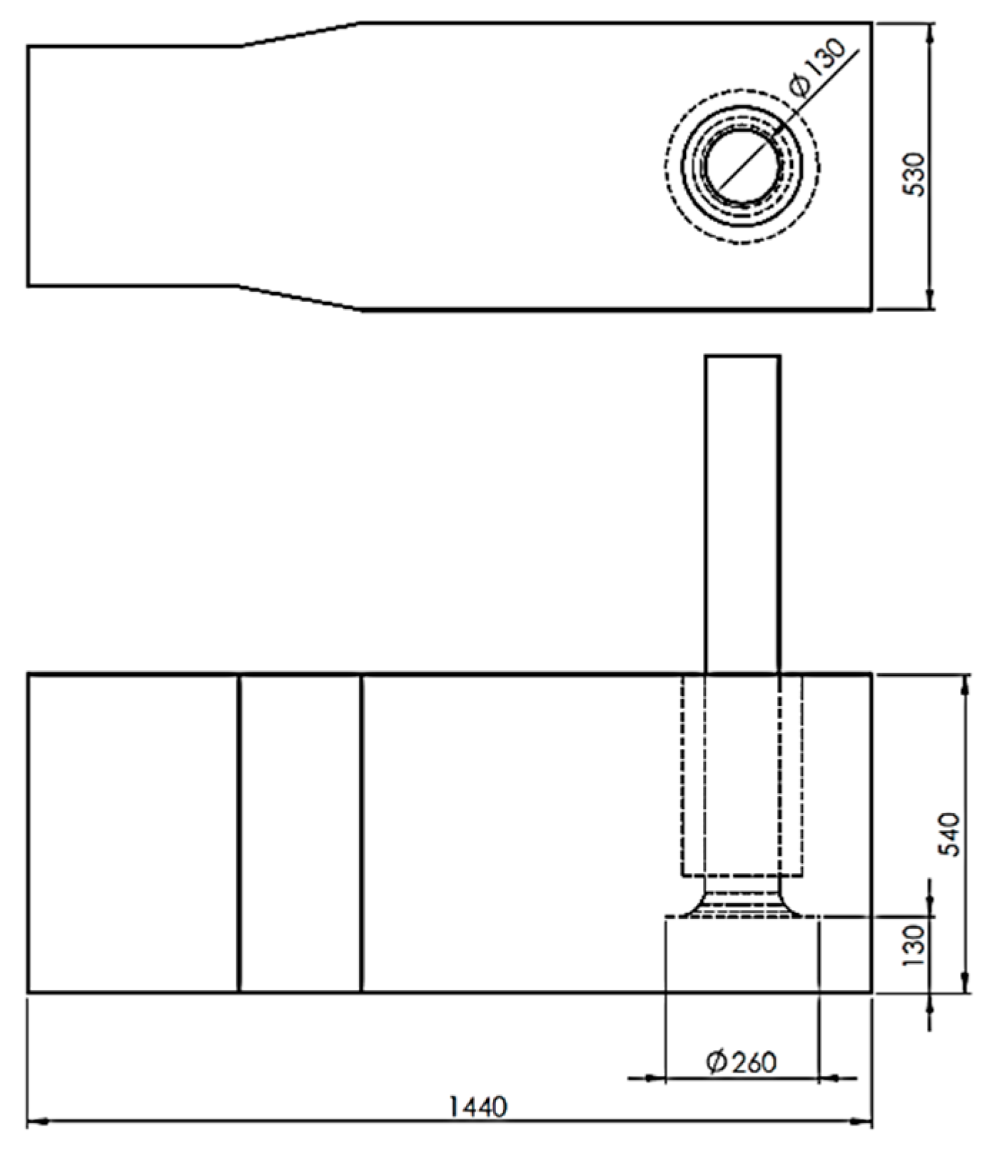
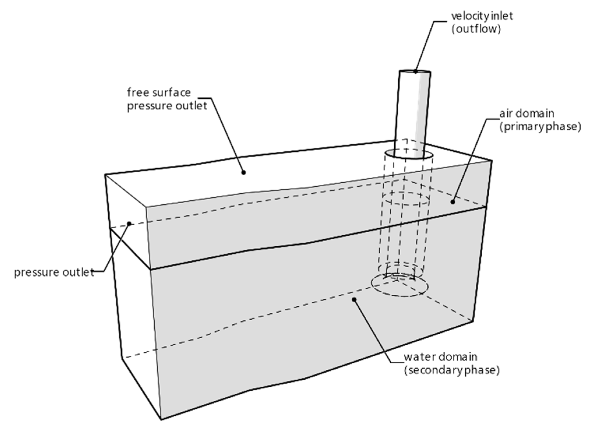
In this study, an implicit volume of fluid (VOF) multiphase numerical model of a 530 mm wide rectangular intake sump housing a 116 m3/h pump with a 260 mm diameter inlet bellmouth is analyzed using ANSYS Fluent. The flow conditions, vortex formation and inlet swirl are compared to the results obtained from a physical model test. The aim of this study is to validate the use of CFD as an alternative method of evaluating flow behavior in pump sumps concentrating mainly on vortex prediction, anti-vortex devices and related prerotation.
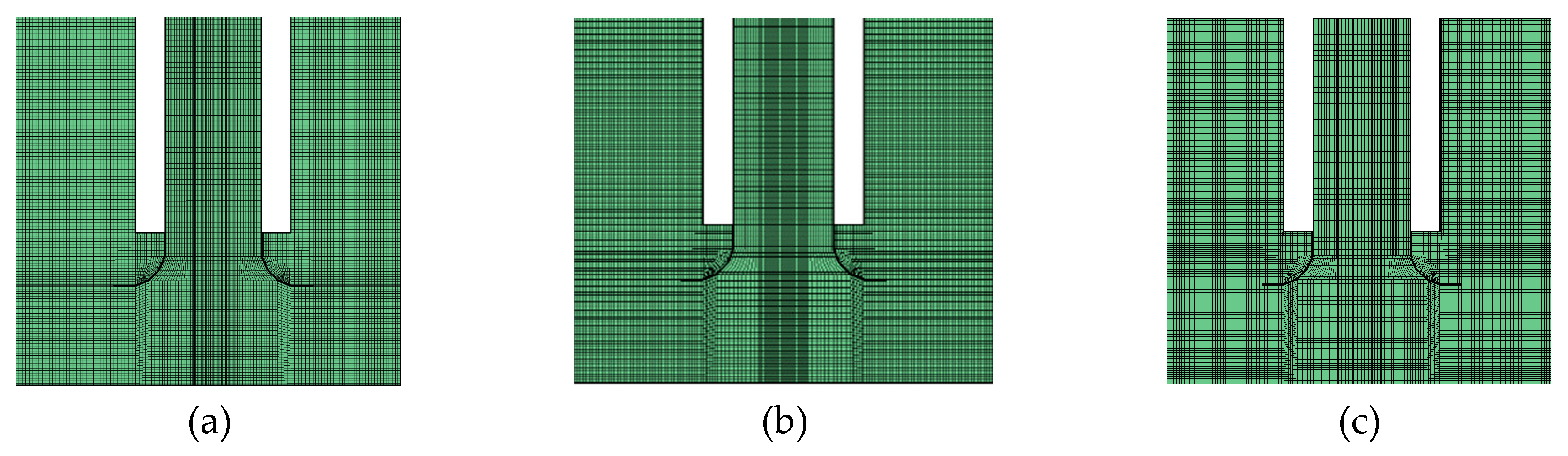
The novelty of this work is the investigation of various sump floor configurations showing their effects on reducing the entrained vortices developed within the suction lines.

2. Experimental Setup

In conducting any CFD simulations, it is vital that numerical accuracy be demonstrated by either comparing results to a well-established analytical model or to the results acquired from conducting a physical model experiment. In this paper, photographs and plot data taken from the baseline test of a 1:10 undistorted scale hydraulic model is presented as reference in evaluating the numerical results. These data are lifted from a recent pump project supplying cooling water to a thermal power plant and are presented here with implicit permission from Hitachi Plant Technologies, Ltd. PBO. (Makati City, Philippines). The prototype model consisted of two 5.3 m wide by 14 m long pump bay and one 2.0 m wide auxiliary channel. The 5.3 m wide pump bay feeds two vertical axis mixed flow pumps each rated at 36,700 m3/h with a total dynamic head (TDH) of 15 m. The auxiliary channel feeds a smaller auxiliary pump rated at 4400 m3/h against a TDH of 12.5 m. For this study, the focus will be on the main pumps since these are the crucial components for this pump station. For open channel flows such as these sump, gravity and inertial forces play a more dominant role than viscous or turbulent shear forces. As such, dynamic similarity during the test was maintained by keeping the Froude number ( F r = 0.38 ) between the model and the prototype constant. Furthermore, ANSI/HI recommends a minimum value for both the Reynolds number ( R e ) and Weber number ( W e ) to avoid any scale effects and surface tension effects in the model. A minimum R e is necessary in order to ensure that the flow condition in the model is as turbulent as that of the prototype. While a minimum W e is recommended in order to avoid surface tension effects particularly in fully developed stage where the vortices start to draw in air from the surface. Table 1 shows the R e and W e numbers calculated at the 260 mm diameter suction bell. These values justify and prove that the selected scale (1:10) is sufficient for the physical model test. Using this scale, the model capacity based on the 36,700 m3/h maximum flow capacity of the prototype is taken as 116.07 m3/h.
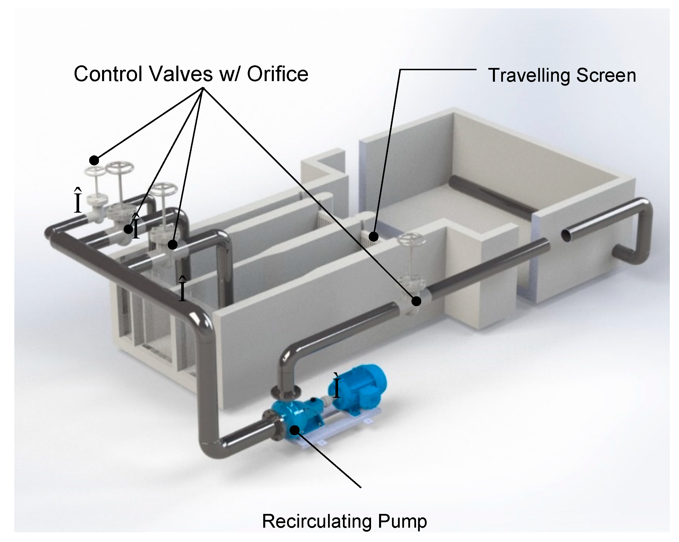
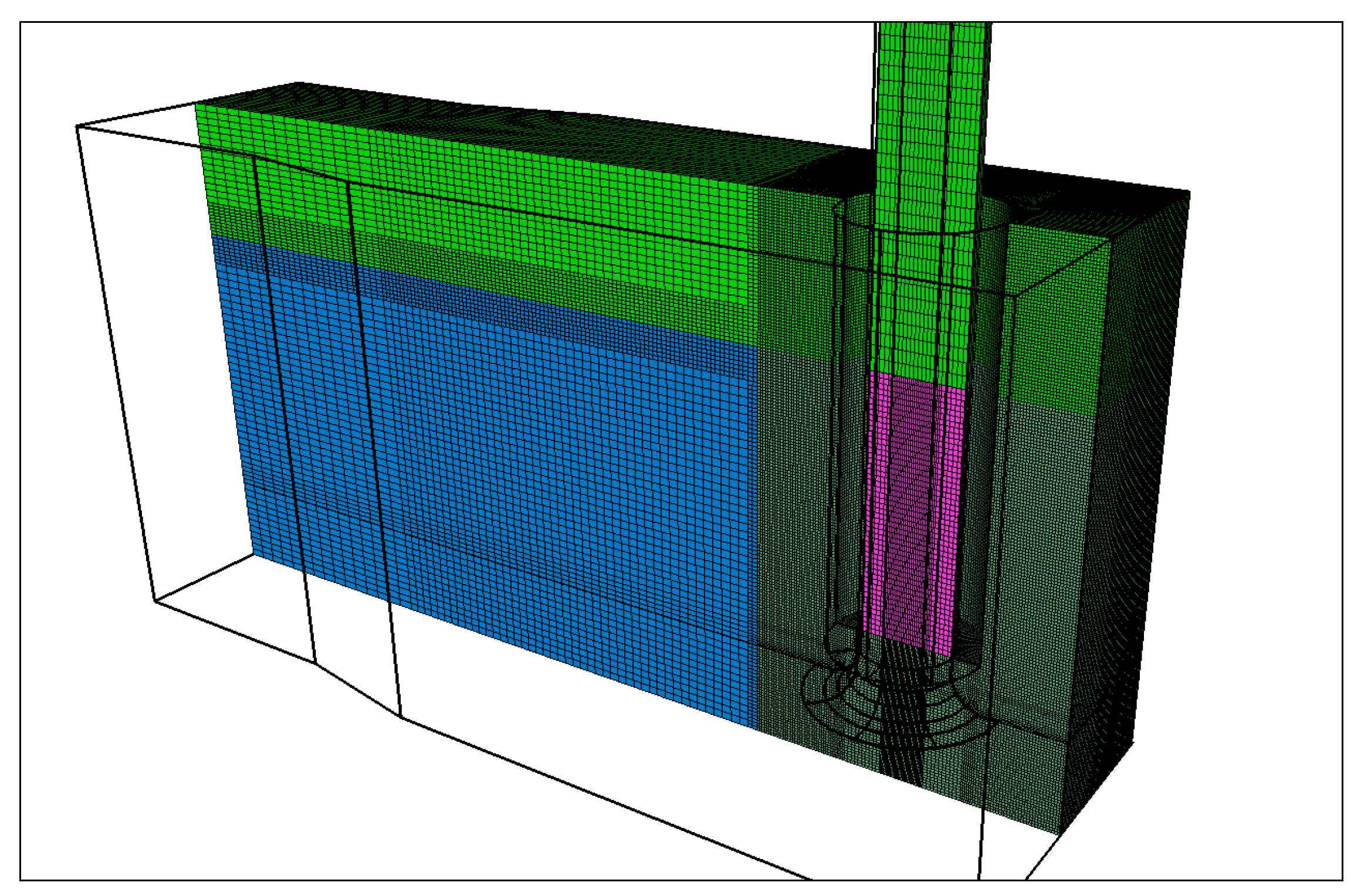
In order to protect proprietary data, a 3D representation of the hydraulic test model is presented in Figure 1 in lieu of a picture of the actual setup. A centrifugal pump was used to recirculate water through a diffuser that spreads the flow over the entire width of the forebay. Orifice plates and control valves were installed to control the individual pump flows as well as the total model flow. Straightening devices were installed in the model head-box representing the trash racks and travelling screens in the prototype. This is to ensure that flow entering from the forebay is as uniform and as steady as possible. Typically for hydraulic model studies, impeller induced flows are not considered. This is mainly due to the fact that the main focus of the test is to verify the flow conditions and vortex formations in the sump as the fluid enters the pump and not the performance of the pump. Hence in this case, the 116 m3/h vertical axis semi-axial pump is represented using a 130 mm diameter vertical pipe with a 260 mm diameter suction bellmouth. The bellmouth was fabricated from transparent polyvinyl chloride to facilitate visual observation.
All other aspects of the hydraulic model test comply with the latest ANSI/HI 9.8 test standards in terms of acceptance criteria, scale selection, data collection and instrumentation. Specifically, the pump model flow rates were determined using an ASME standard orifice meter with an accuracy of ±2%. The water level in the pump sump were recorded with a staff gauge referenced from the sump floor with a minimum accuracy of 3-mm. Velocity probe with a repeatability of ±2% was installed to measure point velocities at specific points along the throat of the suction bell. Typically, measurements of swirl in sump model test are done through visual inspection. The number of revolutions made by the swirl meter are counted and related to the flow rate. For the physical model test discussed in this paper, a swirl meter consisting of four straight vanes mounted on a shaft with low friction bearings was installed at a height of four suction pipe diameters downstream from the bell mouth to measure the level of pre-swirl as flow enters the pump.
The swirl angle is calculated by:
θ = tan 1 ( π d n u )
where u = average axial velocity, d = diameter of the pipe in which the swirl meter is installed and n = revolutions per second of the swirl meter
The design specifications for the physical model is outlined in Table 2.

3. Numerical Model

In order to validate the suitability of CFD in predicting flow patterns and vortex formation in pump sumps, the conditions used for the hydraulic model must be exactly replicated in the numerical model. As such, the numerical models used in this paper are also a 1:10 undistorted reduce scale model of the prototype. Parameters such as flow capacity and water level were also based on the variables used for the hydraulic model test. The only difference is that for the CFD simulation, only one pump bay was modelled due to the symmetrical layout of the sump. The auxiliary pump is operated separately during both the hydraulic model test and during normal operating conditions. This means that the auxiliary pump will not cause any cross-flow during the test or during normal operating conditions. Also, it is expected that both sumps will perform similarly during operation justifying the use of only one pump compartment for the CFD analysis. The total water volume was dimensioned to mirror the low water level ( L W L ) used in the hydraulic model test while the air volume above the free surface of the water was set at a height of 200 mm. The sump dimension and pump location used for the numerical model are shown in Figure 2. For all cases, the numerical solutions for the Reynolds-Averaged Navier-Stokes (RANS) equations were performed using ANSYS Fluent 2019. Turbulence flow properties were described using k - ω Shear Stress Transport model. The free surface is tracked by means of the Volume of Fluid (VOF) multiphase model.

3.1. Boundary Condition and Solver Parameters

Boundary conditions were calculated based in a total flow of 116 m3/h and with a water level of 540 mm. A velocity flow inlet with negative velocity magnitude (outflow) was prescribed as outlet boundary condition at the end of the discharge pipe. The rectangular section serving as the entry point for the sump was prescribed as a pressure outlet boundary condition. Multiphase open channel condition is also prescribed on this surface with the pressure specification method set as free surface level. The free-surface level is set at 0.542592 m and the bottom level set to 0 m. Backflow pressure is specified as total pressure. The boundary condition for the air surface 200 mm over the water surface was also specified as pressure outlet boundary with zero backflow volume fraction indicating that only air can pass through this boundary. Figure 3 shows an overview of the boundary conditions as used throughout the analysis. No slip velocity conditions were used at the walls. Boundary roughness was not taken into consideration since walls were assumed to be smooth. For the purpose of this study, a constant value for density was specified for the entire model. The free-surface level was set as the reference pressure location (0.542952 m) and the specified operating density fixed as 1.225 kg/m3. Calculations were carried out using Eulerian multiphase volume fraction method (VOF) transient conditions with water at 25 °C as the secondary phase and air as the primary phase. The effect of surface tension along the interface between each phase is added in the VOF model by specifying a constant surface tension coefficient (71.2 mN·m−1). Flow is incompressible and isothermal with constant fluid properties. Turbulence was modelled using the k - ω shear-stress transport (SST). SST k - ω had been found to be suitable for numerical modelling of free-surface vortices [19,20] and exhibits better performance in predicting flows at walls and adverse pressure gradients as compared to other eddy-viscosity models [21]. The pressure-based coupled solver was applied. Second order discretization scheme were used for pressure, momentum, and turbulence equations. Converged solution from a steady state simulation was used for the initial conditions. The non-iterative time-advancement (NITA) scheme was used for temporal discretization. This scheme speeds up transient simulations by performing only a single outer iteration per time-step. Overall time-accuracy is preserved not by reducing the splitting error to zero but instead by maintaining it in the same order as the truncation error [22]. The initial time step has been as chosen as 0.001 s, small enough to ensure the correct vortex generation and convergence.

3.2. CFD Mesh Generation

Of primary importance in this study is the flow pattern around areas with high velocity and high velocity gradient like the suction bellmouth and the free surface just above the suction pipe. This area is where vortices are expected to occur during operation thus focus is given to the mesh size and quality within these areas in order to ensure accurate results. The initial attempt to model the whole structure with a homogenous mesh size yielded a very large model size that easily exceeded the capacity of the current equipment used in this study. As such it was necessary for the model to be divided into four regions as shown in Figure 4. The first region extends from the backwall of the sump up to 220 mm upstream of the pump and covers the full height of the water and air domains. This region effectively covers the bellmouth, the throat and any region where the velocity gradient is expected to be high. The second and third regions contains the discharge pipe and the last region contains the area just upstream of the intake (i.e., forebay).
In order to optimize computational time and study the effect of grid resolutions, a preliminary grid independence study had been conducted comparing results for three CFD models. Additionally, the grid independence study ensures that the results are due to the boundary conditions and physics used and not by the mesh resolution. Three hexahedral mapped meshed models labeled as fine, medium, and course mesh with 1.9, 2.4 and 3.2 million cells, respectively, were generated for this purpose. For the models used in this paper, the mesh refinement didn’t follow the usual half/double element size since refining the mesh by a factor of 2 will result to an 8-fold increase in problem size which is unacceptable for engineering design purposes. The three CFD models differ in the first region which was modelled with three different mesh densities since this is the area where the analysis will be focused on. Since the final goal of this paper is to predict vortex formation, the 2.4 million mesh model was prepared first, keeping the element size between 0.8 to 2 mm near the suction bell and free surface. For the other regions with lower velocity gradients and where knowledge of the flow pattern was not so important in the analysis, a courser and similar mesh was applied so as to reduce overall computational time. Non-overlapping mesh interfaces were adapted in ANSYS Fluent to combine the three regions and independence between areas with different mesh densities were improved by using the automatic mesh refinement tool feature of the software. In this case, two to three mesh layers were automatically redefined providing an improved 4:1 cell face ratio between the master and the slave faces. A higher and more uniform element count could had been generated but it should be noted that this paper focuses on an optimized method that would result in reduced computational efforts in order for CFD to merit its use in industrial applications. A cross sectional view of the course, medium and fine meshed models are shown in Figure 5.
For the mesh independence study, it is crucial to have a prior knowledge of the flow phenomenon in order to apply the correct solution methodology. In this case, during the hydraulic model test, it was observed that the forebay was able to provide steady and uniform approach flow. Also, no significant free surface vortices with air-core were observed under the specified flow conditions. These observations coupled with the simple geometry of the sump makes it safe to consider a steady state solution for the mesh independence study. For all three numerical models, convergence was defined where the mean velocity and the amplitude of the fluctuating field does not vary for more than 1% for each iteration and the target residual errors kept below 10−4. Axial velocity ( z ) at several points along a line just below the entrance of the suction bell (el. = 0.12 m) perpendicular to the flow direction is plotted as shown in Figure 6. Additionally, in Figure 7, the velocity distribution along a central line that runs parallel to the flow direction and at 0.12 m elevation from the sump floor is plotted for all 3 numerical models. Based on these plots, the simulation results qualitatively show the same structure with the point velocities showing a maximum variation of 0.5% from the average velocity value occurring at the center of the suction bell as expected. The resemblance of these plots for all three cases shows that these simulations can be considered relatively grid-independent based on the presented mesh densities. Generally, for such cases, the coarse mesh is the best alternative for succeeding simulations in terms of minimizing computational time but in this paper, considering how close the results are between the fine mesh and the medium size mesh, and to more fully resolve both the free-surface vortices and submerged vortices originating from the bottom and sidewalls of the sump, the medium sized mesh model was used.

4. Results and Discussions

4.1. Approach Flow Pattern

For the physical model test, the hydraulic behavior in the sump were assessed by measuring the swirl-angle and by observation of the flow patterns and vortex phenomena. The approach flow condition from the forebay entering the pump compartment were uniform and stable as indicated by the dye patterns in Figure 8. Even though pre-swirl is slightly high and unsteady, the flow from the far end is stable and approaches the pump without much turbulence. Dead water zones were not observed.
Similarly, for the numerical model, the approach flow pattern for the sump is steady and uniform as shown in Figure 9. No unwanted swirl or circulation as water flows from the inlet of the domain and towards the suction bellmouth. This flow pattern is identical to the pattern observed during the physical model test previously. This verifies that the selected forebay length for the numerical model is sufficient in providing a stable velocity gradient from the inlet of the domain without any unnecessary turbulence which could influence any free surface or subsurface vortex formation downstream of the forebay.

4.2. Free Surface and Sub-Surface Vortex Prediction

Figure 10 shows the presence of a strong floor vortex activity during the physical model test. In general, this phenomenon is expected given the absence of any floor cone. For this model, the vortex is a stationary type 2 vortex. In other installations, stronger and more dangerous floor vortices may be observed. This is when the pressure near the suction bellmouth falls below vapor pressure producing an air-core to develop at the center of the vortex which makes its way towards the impeller. Submerged vortices are very sensitive to the floor clearance or the distance of the suction bell mouth from the sump floor. One solution is to increase this floor clearance, but oftentimes, this solution inadvertently produces dead zones below the pump, hence an alternative solution is required to suppress this phenomenon.
Similarly, intermittent type 2 sidewall vortex activities were also observed as shown in (Figure 11) while stronger vortices which occasionally develop to type 3 were observed on the backwall (Figure 12). The backwall vortices were stronger because of some instability behind the pump. The flow drifts from side to side and then switches directions as shown Figure 13. This may be attributed to slightly larger backwall clearance (2.5 m) in the pump as compared to the recommended value of ANSI/HI 9.8 (1.95 m). Also, the sidewall vortex combined with the floor vortex significantly increases the swirl in the pump suction pipe.
On the surface of the sump, type 1 to type 3 free surface vortices were also observed during the test. Figure 14 shows a surface vortex developing from a surface dimple (type 1) to a full dye-core (type 2) and then dissipating. Due to their transient nature, the vortices form and dissipate without any predictable pattern. For the given flow condition and submergence, the vortices were too weak to draw in some air and/or debris (type 4). As per ANSI/HI 9.8 criteria, type 3 vortices are allowed only when they occur for less than 10% of the 15-min test duration. For this particular case, these surface vortices are acceptable and the need for additional modification such as curtain walls or false ceilings are unnecessary.
Using the same flow conditions for the analysis, similar phenomena were observed in the CFD simulation. In Figure 15a, a strong backwall vortex is represented by the swirling streamline. It can be seen that at the backwall, there is downward flow towards the center of the sump from two separate directions. This causes the flow to form a strong swirling pattern (Figure 15c) just behind the pump which consequently leads to an organized submerged vortex.
Likewise, similar conditions can be seen in Figure 16 for the sidewall and floor vortices. It is observed that as flow is forced to rotate behind the pump, circular eddies are created in the dead spots allowing vortices to form as the flow separates from the walls of the sumps. This flow separation is what contributes to the swirling motion as the fluid enters the bell mouth.
Lastly, Figure 17 below shows the CFD results for the sump wherein the presence of a surface vortex is indicated by the tight curling streamlines. It can be seen the dominant free-surface vortex matches perfectly to that shown in the hydraulic model. It is clearly seen via CFD that the vortex was at most type 3 and was not able to draw in any air as can be seen from the air-volume fraction (3%) isosurface plot in the same figure.
Although the strength of the vortex cannot be accurately determined through the CFD results, a qualitative validation can be made by comparing the location and number of vortices predicted by the simulation with those observed during the physical model test. For this study, it can be seen that numerical results tend to agree with the results of the physical model test.
Based on these results, it is clear that the sump fails to meet the acceptance criteria set forth by ANSI/HI and would need to be optimized based on the following observed hydraulic phenomena:
  • strong type 2 submerged vortex at the floor of the sump;
  • strong type 2 to type 3 submerged vortex behind the pump.
As such, two sets of numerical models are further investigated employing the use of published remedial measures specifically focusing on fillet-splitter designs in order to evaluate performance by improving flow patterns and vortex suppression. Since both the physical model and the numerical model showed allowable intermittent free-surface vortices, the succeeding analysis will be directed towards reducing the formation of sub-surface vortices within the sump.
ANSI/HI 9.8 provides several fillet-splitter designs as a guide for designers in improving sump performance. The most common of which is as shown in Figure 18a employing a trapezoidal cross-baffle along the floor of the sump and a vertical baffle along the backwall. It is important to note however that these recommendation from ANSI/HI are not part of any standards and are not mandatory but instead are presented only to assist engineers in considering factors beyond the standard sump design. Additionally, Figure 18b shows an alternative fillet-splitter design showing a trident shaped floor splitter with triangular profiles along the floor of the sump and 45° chamfers on all corners of the sump near the pump column (sidewall-backwall, backwall-floor, and sidewall-floor corners).
The CFD results (Figure 19) for the cross-baffle splitter design which is based on ANSI/HI 9.8 recommendation shows that the proposed design was not able to suppress the subsurface vortices observed in the unmodified pump sump. Backwall and sidewall vortices were still observed as a result of the flow separating from the walls as soon as it reaches the shortest route to the suction bell.
Conversely, for the trident-shaped fillet-splitter design, it was observed that flow is very stable. The diverging flows on the sidewall as seen in the baseline and initial splitter models were not present in the optimized design as shown in Figure 20. No circular eddies can be observed on the velocity vector plot along the sidewall and flow remains attached to the wall and fillet as it approaches the pump.
Attributed to the increased fillet angle and removal of the horizontal floor splitter, streamlines on all sides of the sumps remains attached to the walls (Figure 21). No flow separation and unwanted swirls. Sub-surface vortices were very minimal and only occurred near the entrance of the suction bellmouth.

4.3. Swirl Angle Prediction

ANSI/HI 9.8 provides two criteria for assessing swirl angle. One is the long-term average swirl angle measured/observed for a 10 min duration. The other is the short-term maximum swirl angle observed for 30 s duration. The sump should not exhibit a swirl angle greater than 5° for both criteria in order to be considered acceptable. Among the two, the short-term maximum swirl angle is the more stringent and problematic criteria since this measurement gives an indication of the instantaneous swirl. For this same reason, the paper focused on measuring the pumps sump’s max short-term swirl angle.
The CFD swirl measurements were taken at the similar location as that of the rotameters in the physical model test. Specifically, at a distance of 503 mm (approximately four times the pipe diameter) from the bellmouth. Figure 22 shows the CFD prediction for the swirl angle for all three sump geometries over a period of 30 s.
For the original unmodified sump geometry, numerical results show a maximum 30-s swirl of 3.75° which is lower than the maximum short-term swirl obtained from the physical model test. Table 3 shows the results obtained from the physical model test. As shown in the table, a maximum number of 26 rotations made by the swirl meter for a 30 s duration was observed. This data, yields a maximum short-term swirl of 7.5°. Similarly, the table shows that about 86% of the time, the short-term swirl angle was observed to be greater than 5°. Similarly, an average of 13 rotations per minute was observed over a 900-s duration yielding an average long-term swirl angle of 1.88°. With regards to the maximum short-term swirl angle, the discrepancy between the numerical and the experimental results may be attributed to the difference in the measurement method used between in the physical model test and the CFD analysis. The physical model test measures swirl angle using a rotameter which can change rotation direction depending on the flow. In general, any change in direction of rotation introduces errors or uncertainties in determining the average causing a lower observed value. On the contrary, assuming correct tangential and axial velocities, CFD results provides exact average conditions.
For the initial and optimized splitter designs, the CFD predicted maximum swirl is 3.4° and 2.9°, respectively. If these values are considered, since ANSI/HI 9.8 mandates that both the short-term maximum and the long-term average swirl angle should not exceed 5°, it may be inferred that both fillet-splitter design meets the criteria for acceptable swirl angle.

4.4. Point Velocities

For the physical model, the velocity profiles are measured by means of velocity probes installed at the throat of the suction bellmouth. Figure 23 shows the velocity profile as measured across the plane of the impeller eye.
The spatial variation varies between −4.0% and 3.6% of the mean velocity indicating that the flow velocity for the unmodified sump falls within the 10% acceptance criteria.
Similarly, for the numerical models, temporal velocity profile taken for a period of 30 s for the same points monitored during the physical model test are shown in Figure 24. The spatial variation for all three cases varies between 0.4% and 4.8% of the mean velocity indicating that the flow velocity for all the sump geometries is within the acceptance criteria. In comparison, it can be seen that the CFD results were able to match the trends and the magnitude of the axial velocities as obtained from the physical model test.

5. Conclusions

This paper presented results of numerical simulation as compared with data from reduced-scale physical model test of pump sump focusing on vortex prediction and swirl angle at intakes.
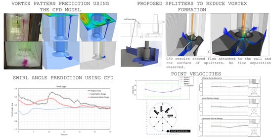
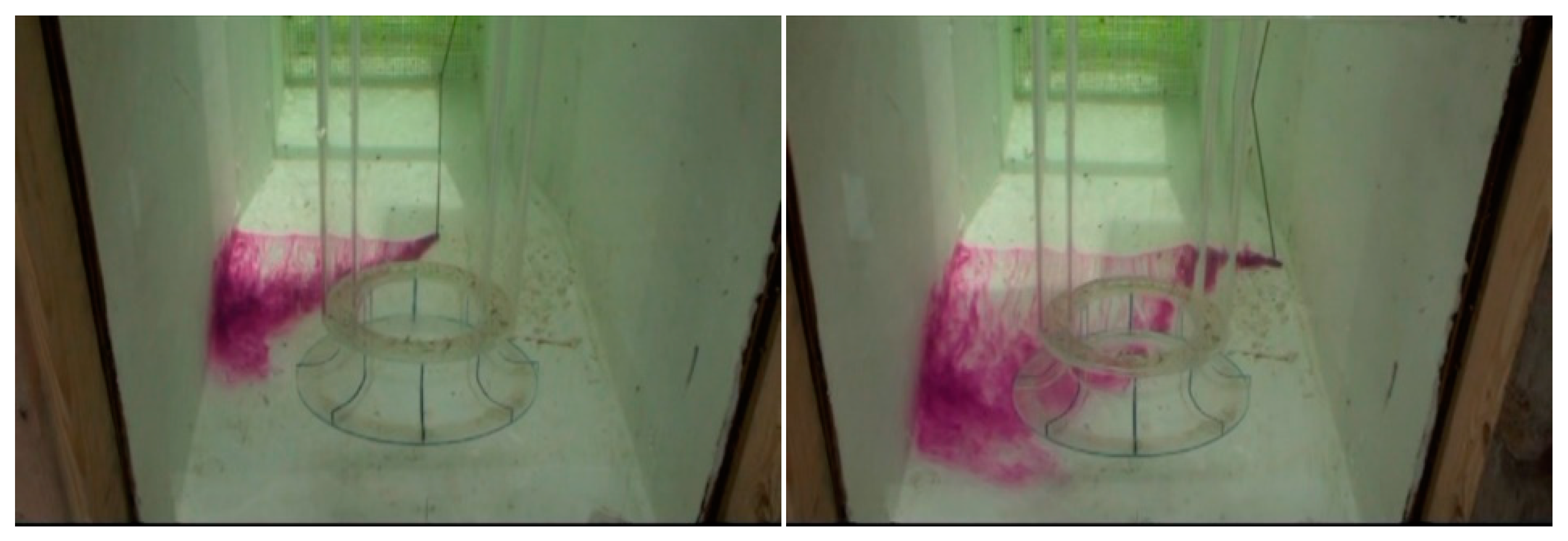
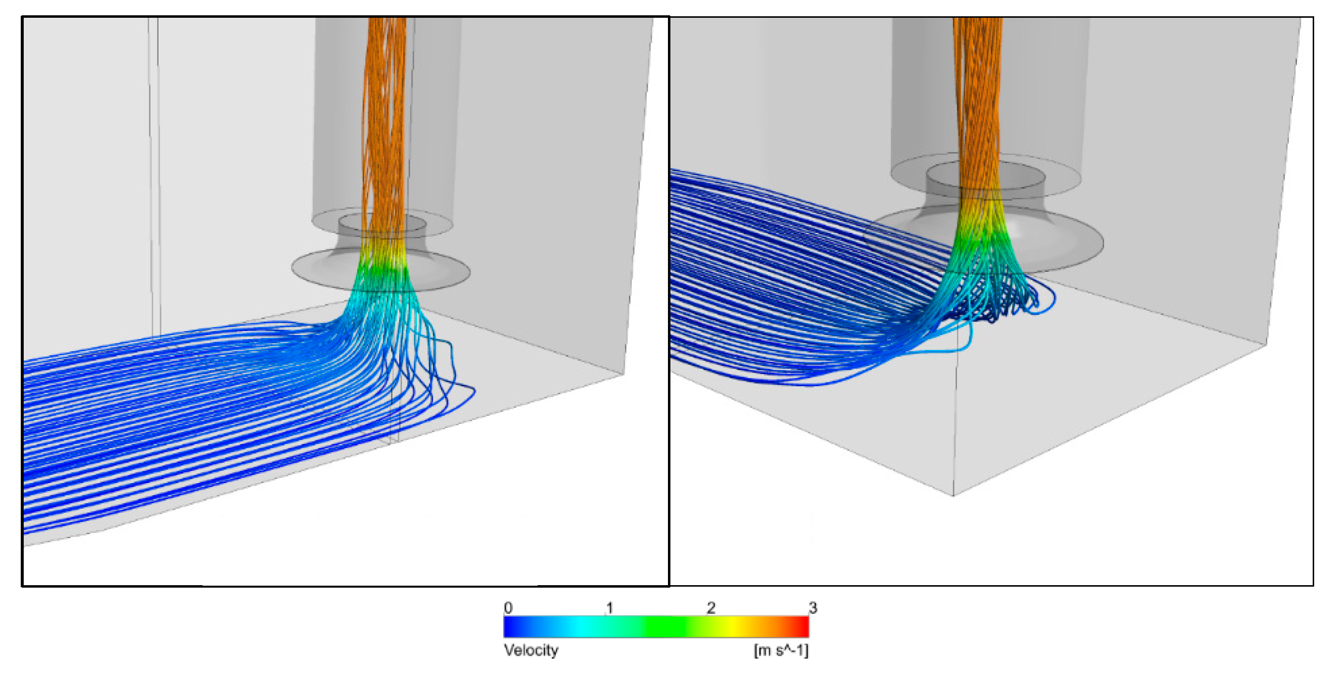
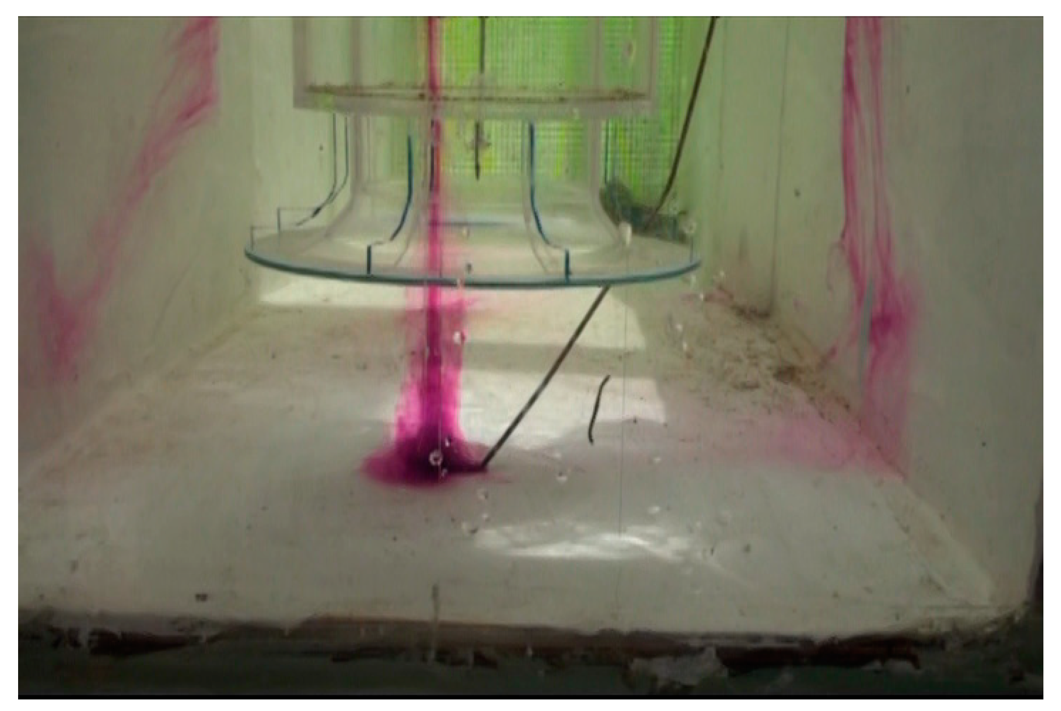
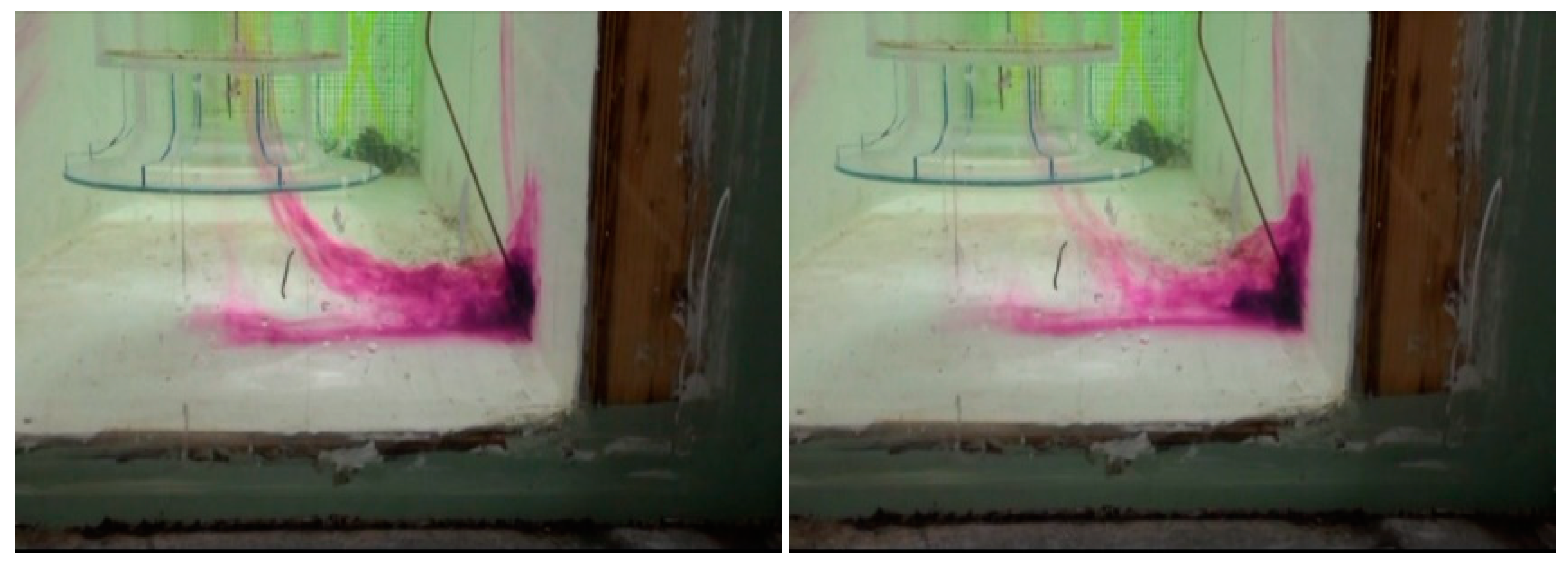
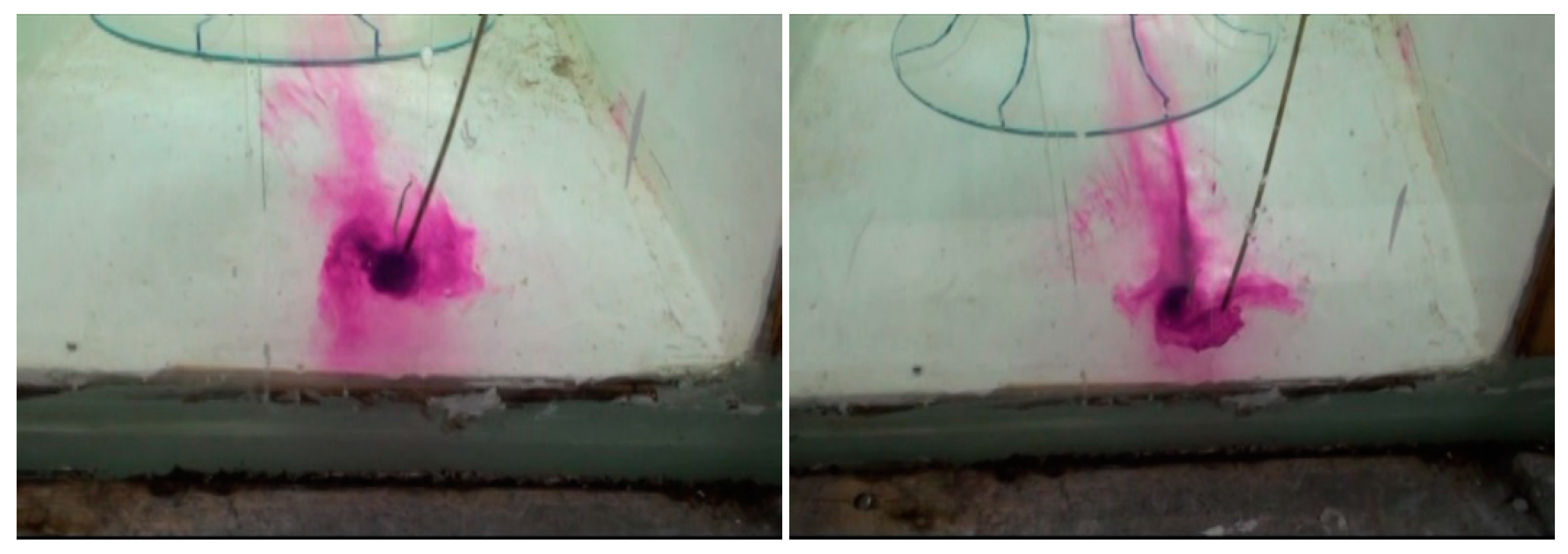
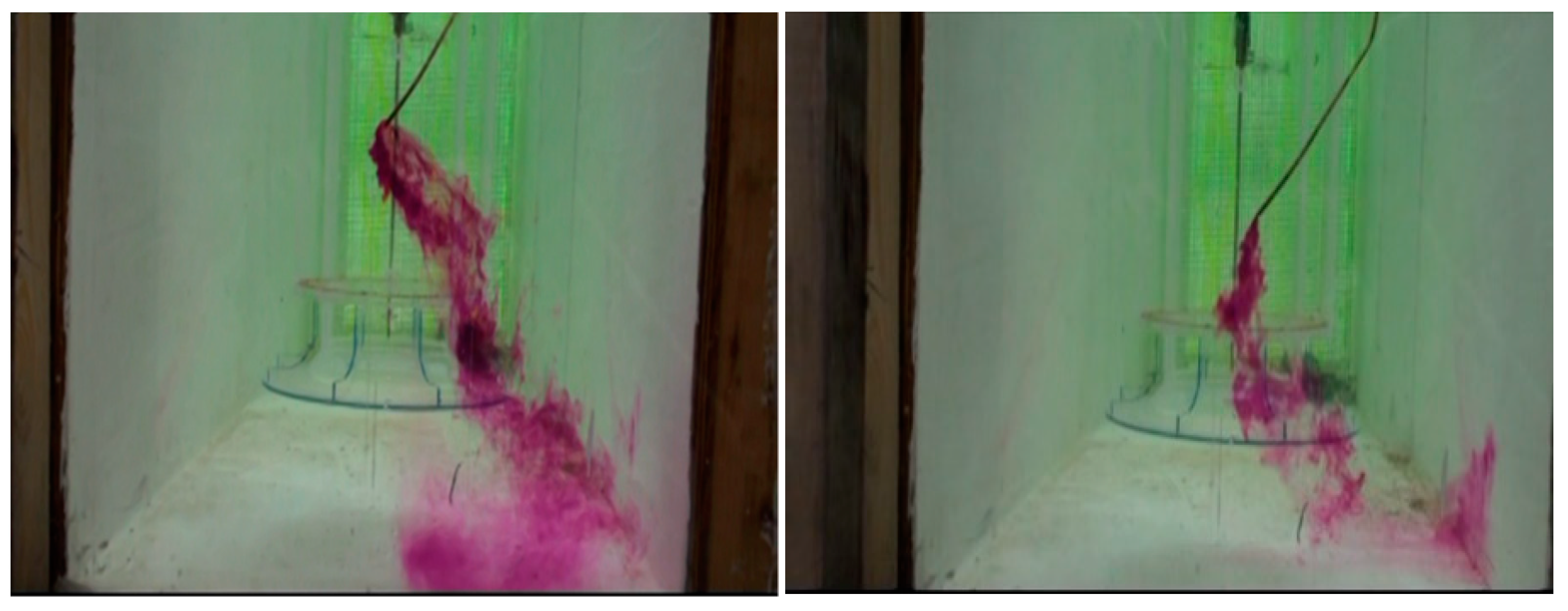
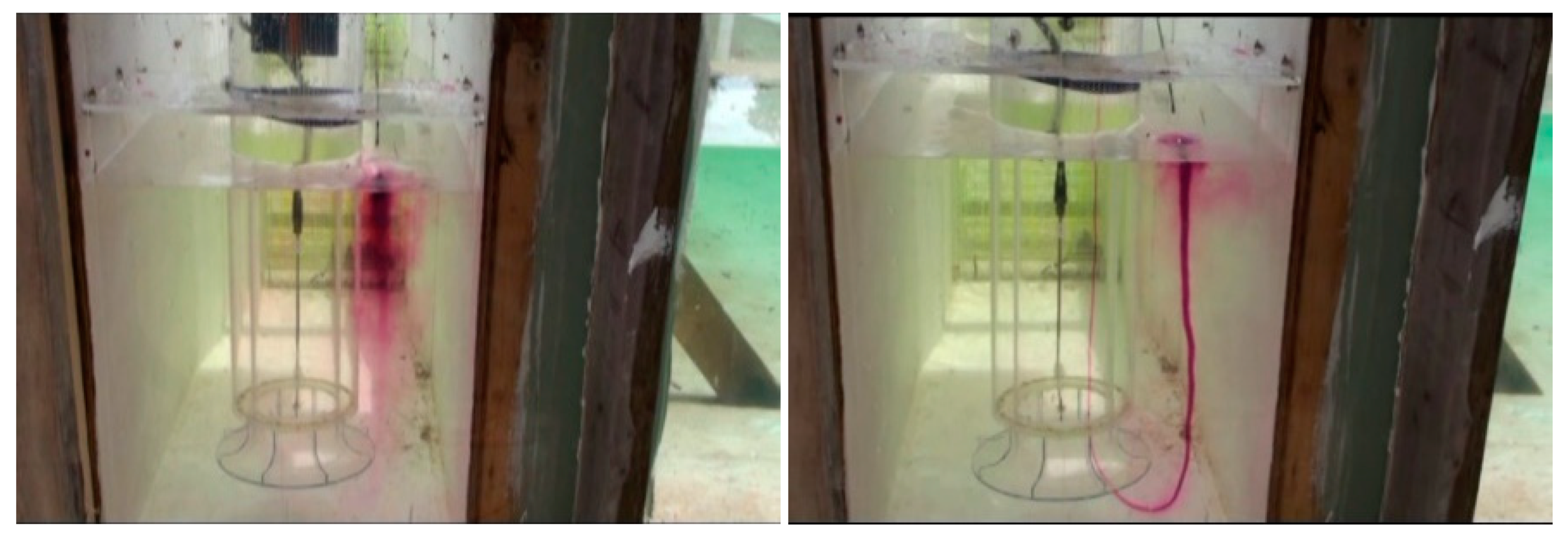
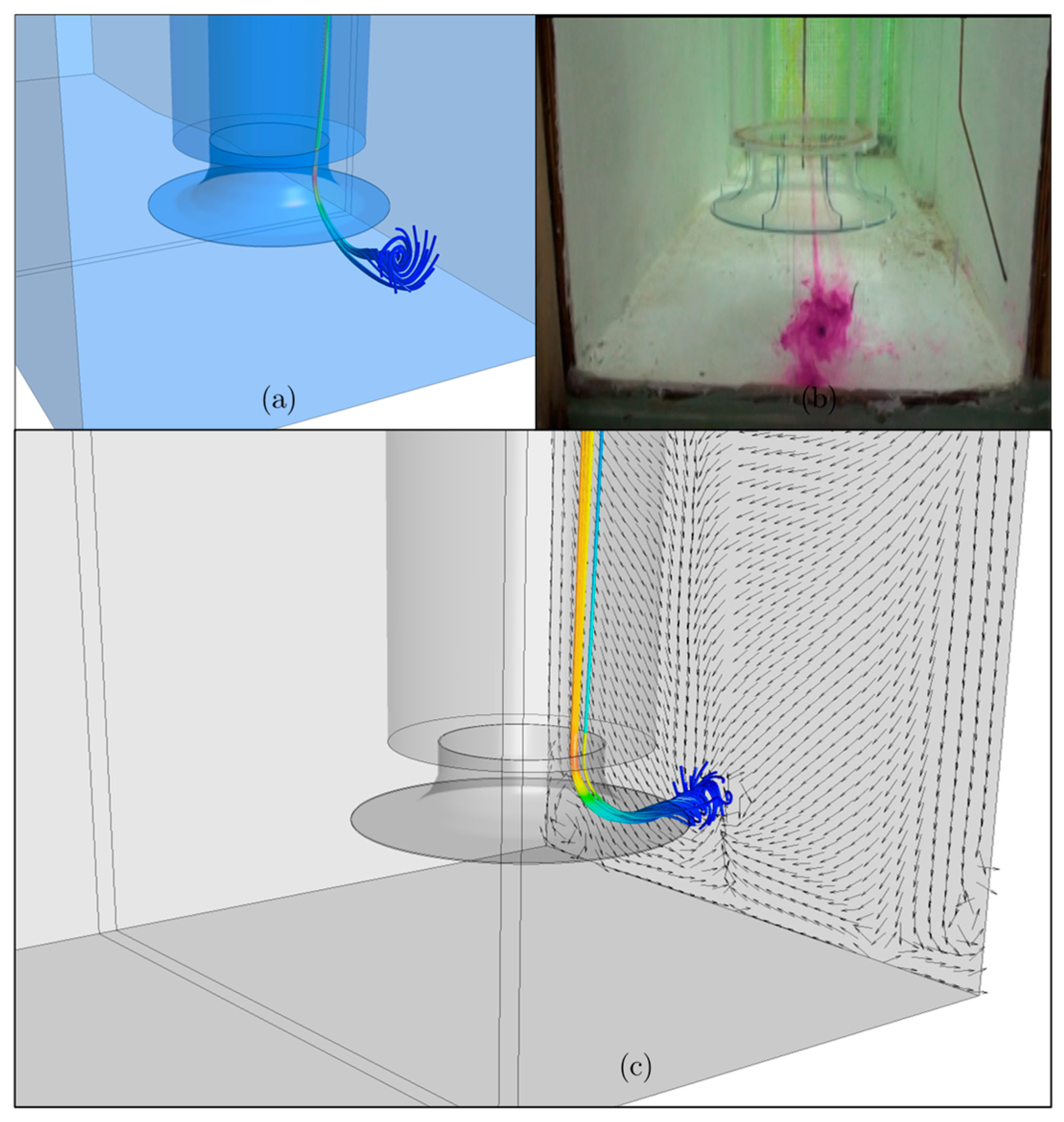
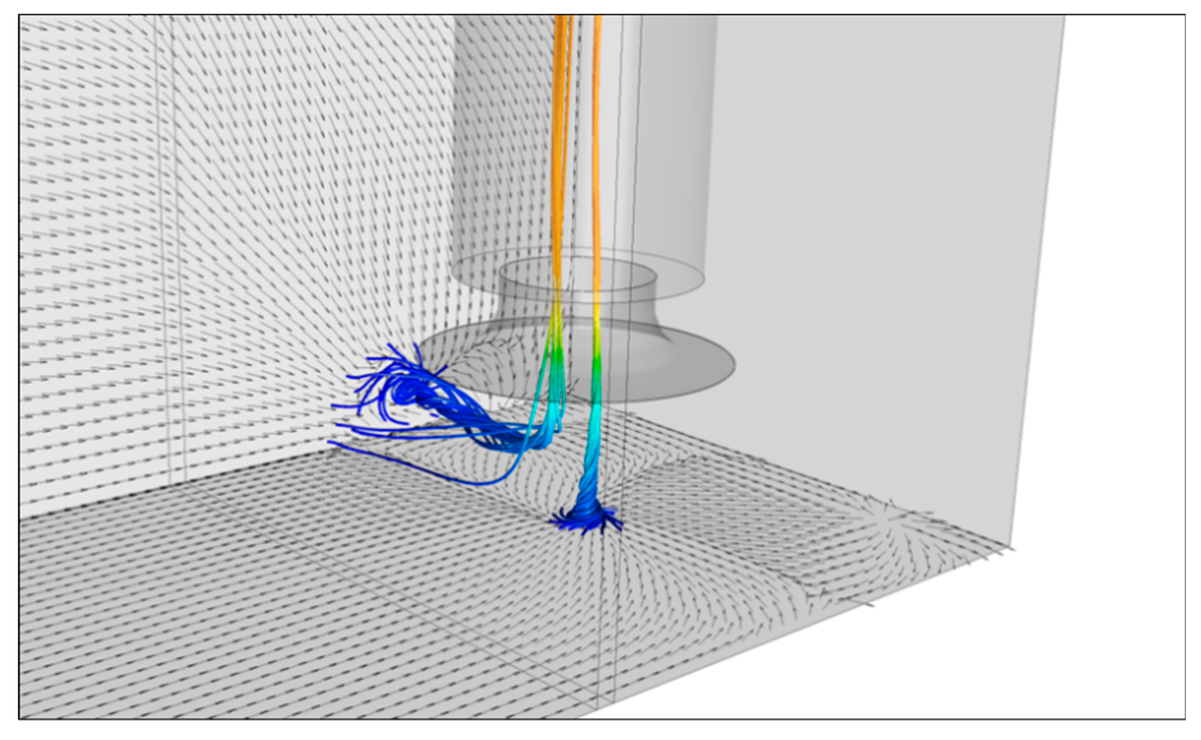
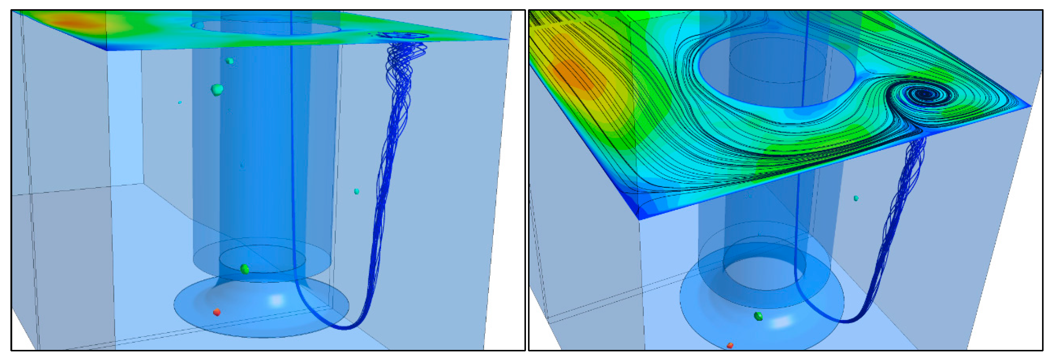
The numerical model was able to accurately predict the formation, size and location of the type 3 surface vortex that was observed in the physical experiment. Similar to the experiment, the predicted surface vortex was intermittent and was not able to draw in any air to the suction bell mouth.
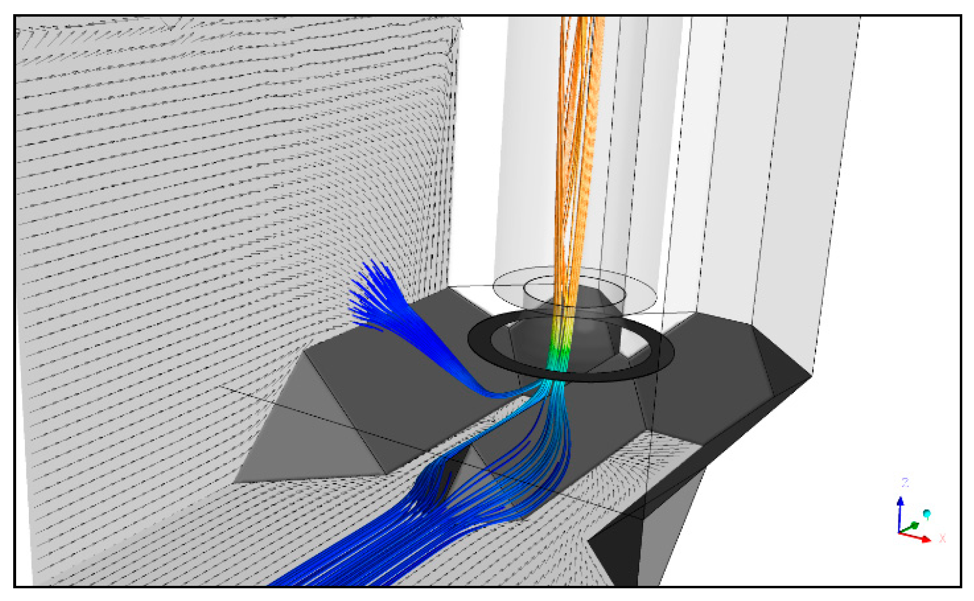
The strong backwall and floor vortices observed in the physical model test were also replicated in the numerical results. Numerical results showed that the flow separation along the side walls of the sump as well as high turbulence at the back of the pump to be the primary cause of this submerged vortices.
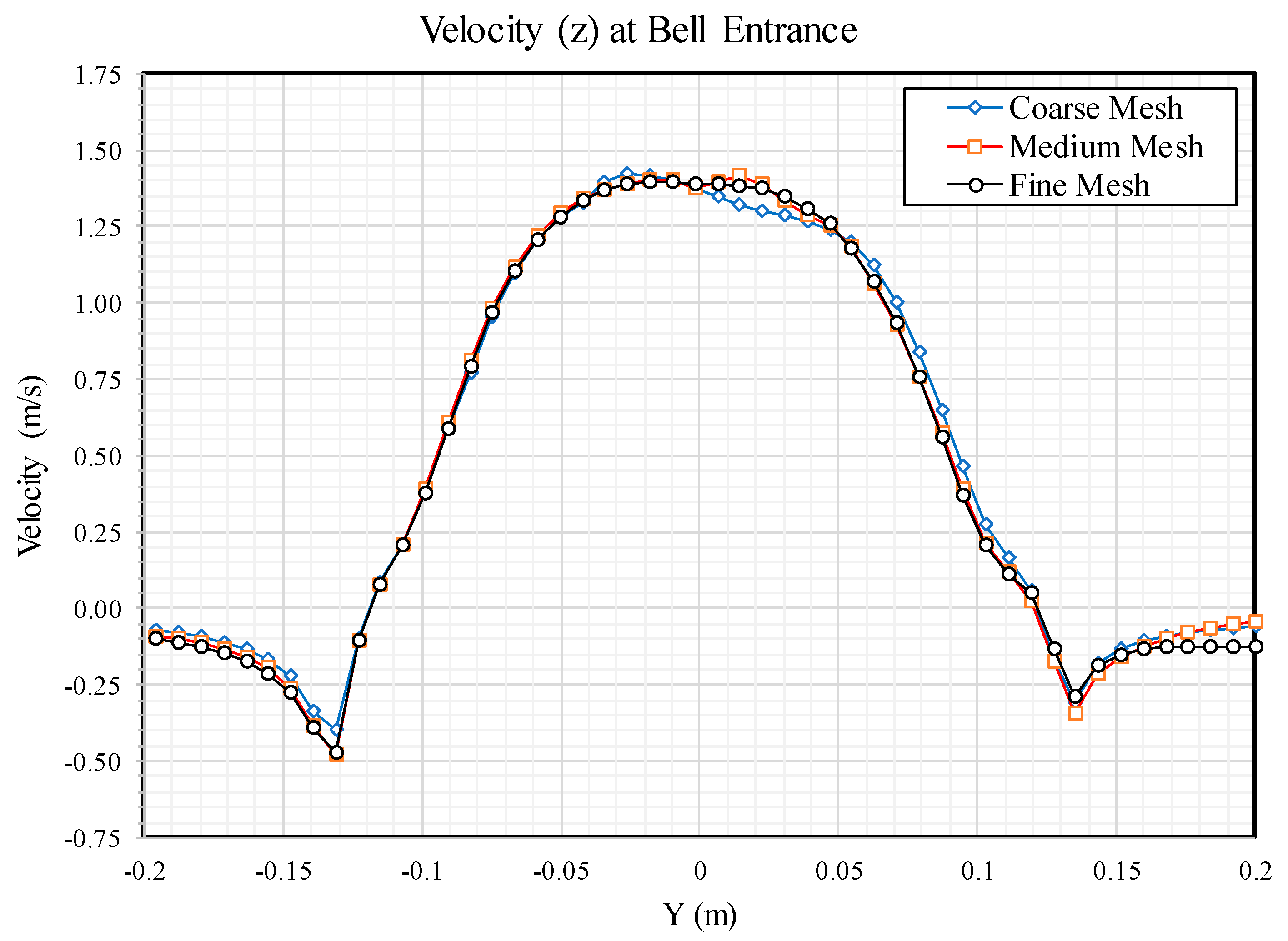
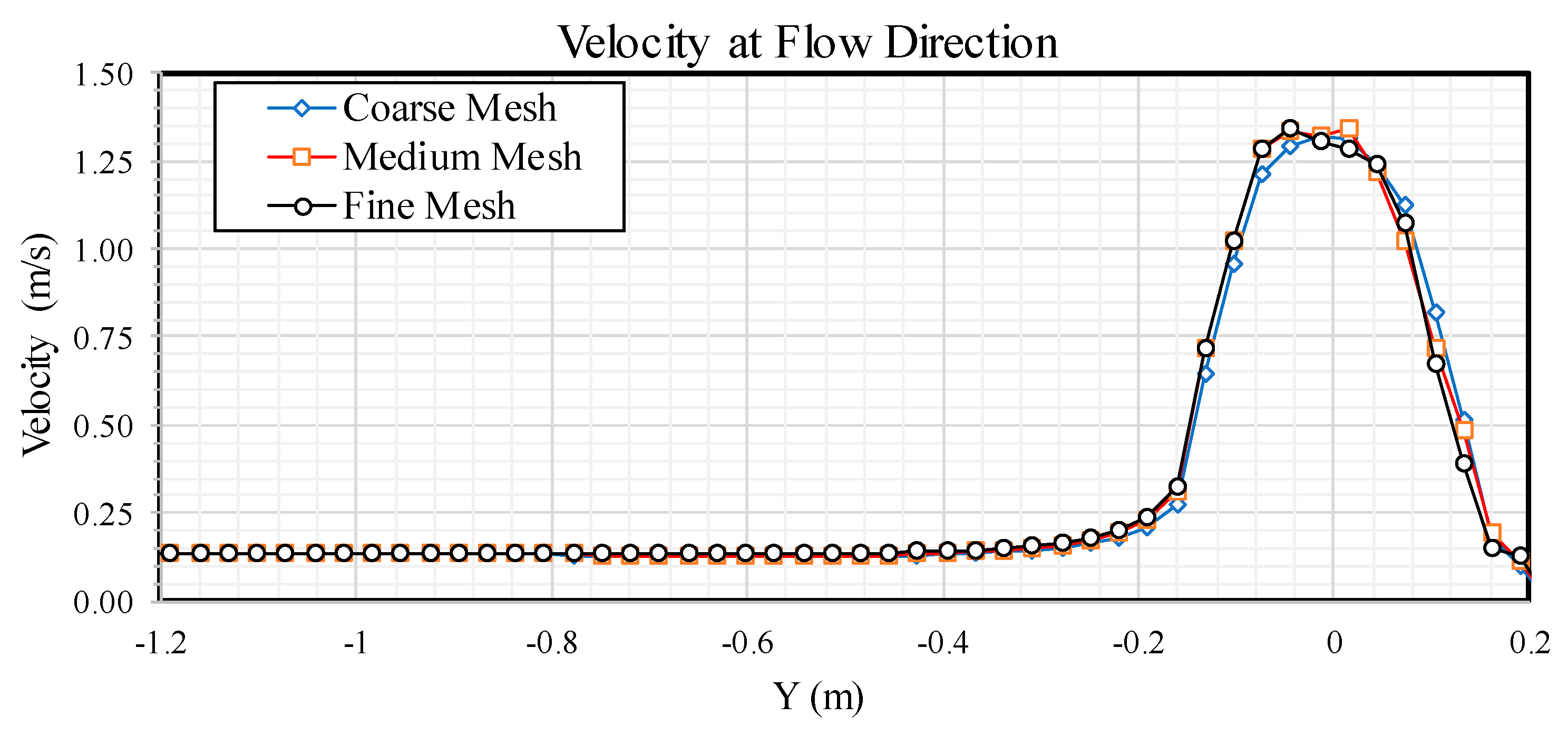
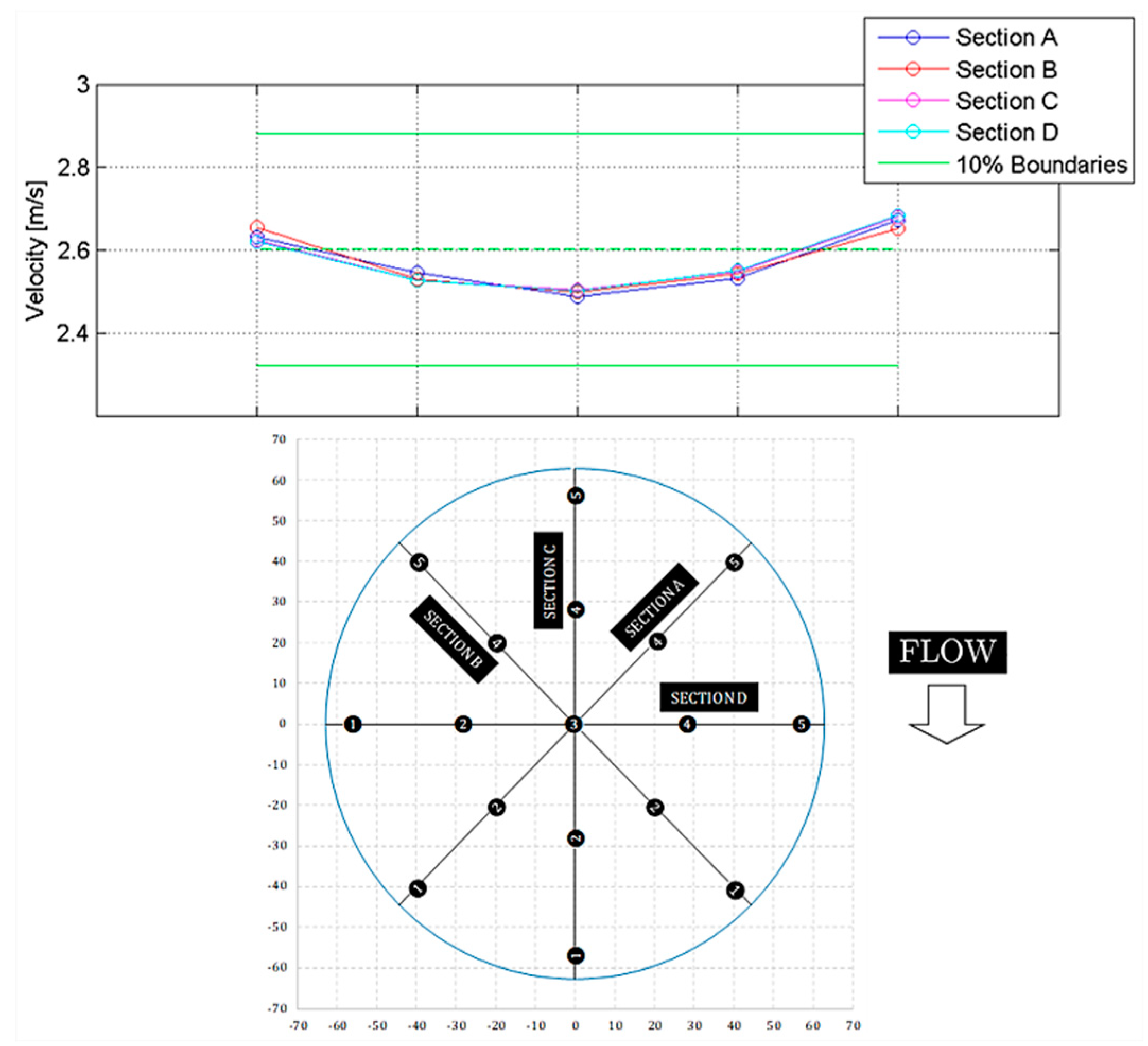
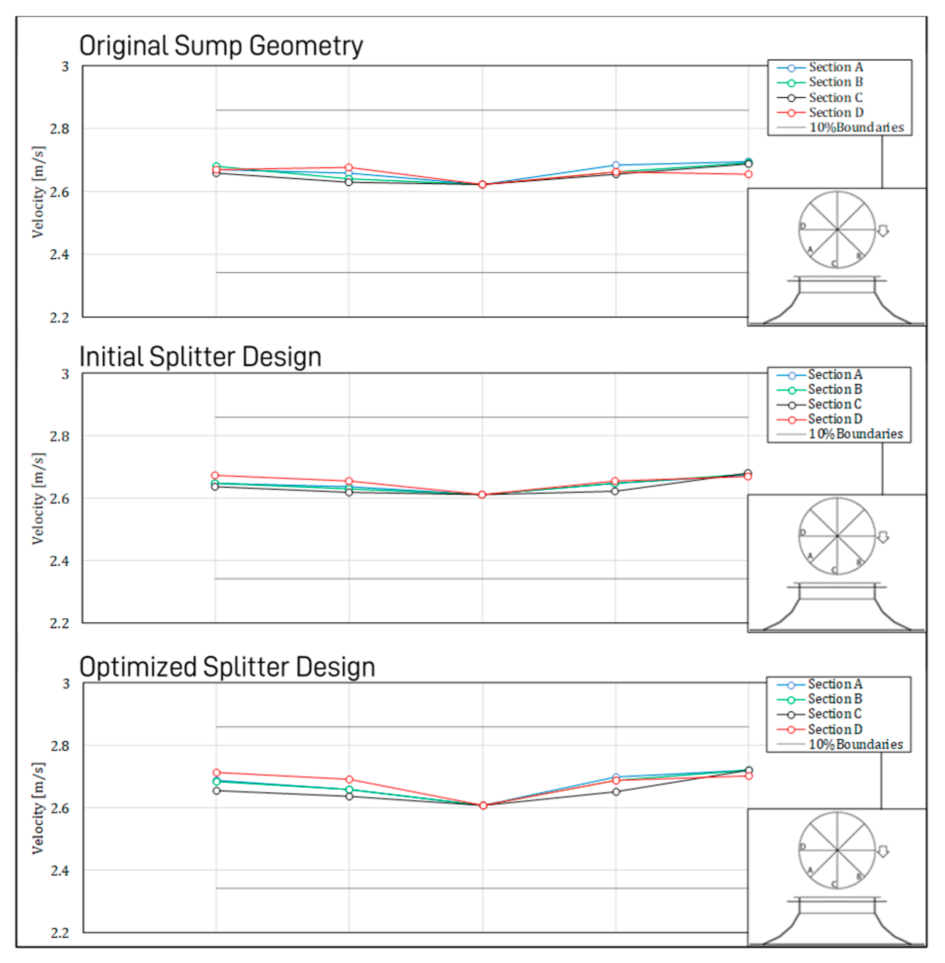
Point velocity data from the numerical analysis showed a good agreement with those measured at several points along the bellmouth throat during the physical model test. Both numerical data and experimental data displayed acceptable similarity in terms of magnitude and trend.
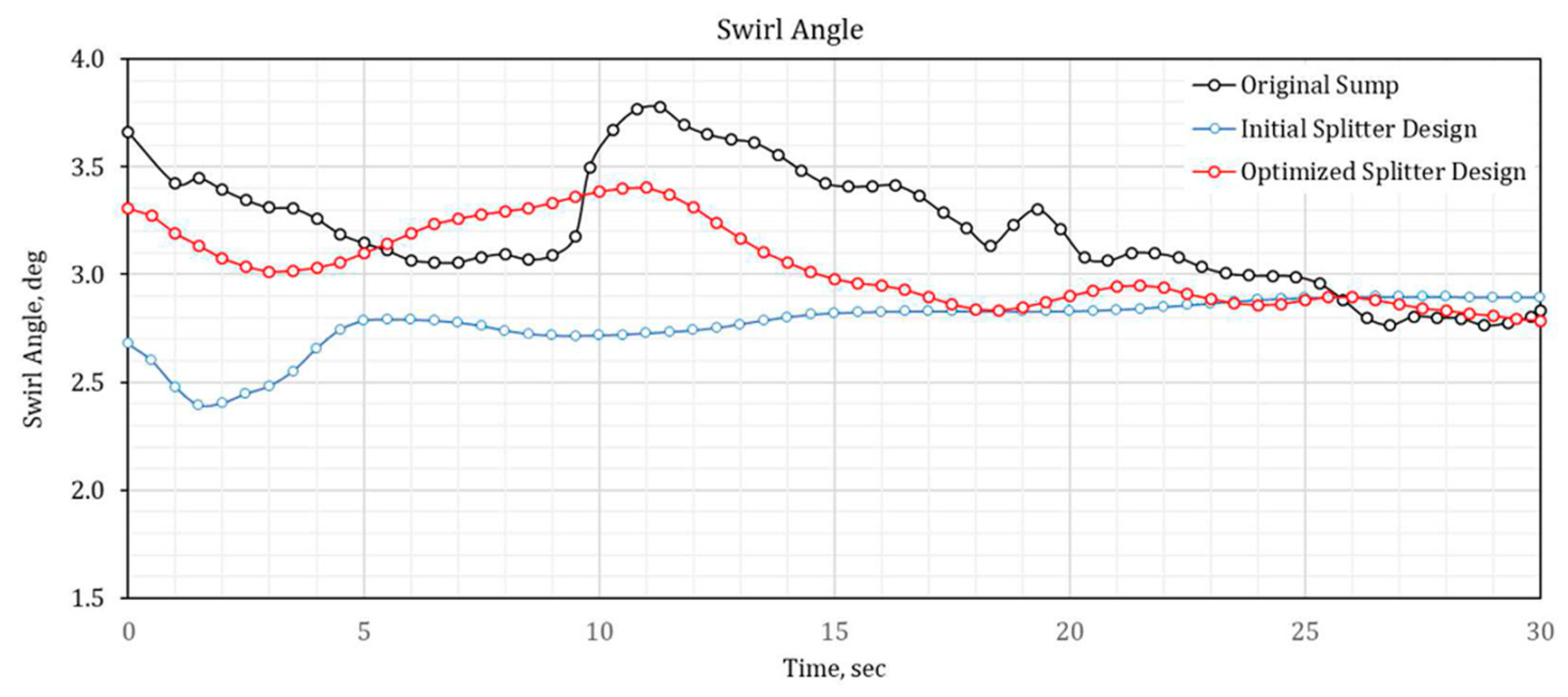
On the other hand, numerical results showed a 30-s maximum short-term swirl angle of 3.75° at a location where the pump impeller was supposed to be. This value is lower than the maximum short-term swirl of 7.5° obtained from the physical model test. The discrepancy between the numerical and the experimental results may be attributed to the difference in the measurement method used. The physical model test measures swirl angle using a rotameter which can change rotation direction depending on the flow. In general, any change in direction of rotation introduces errors or uncertainties. On the contrary, assuming correct tangential and axial velocities, CFD results provides exact conditions.
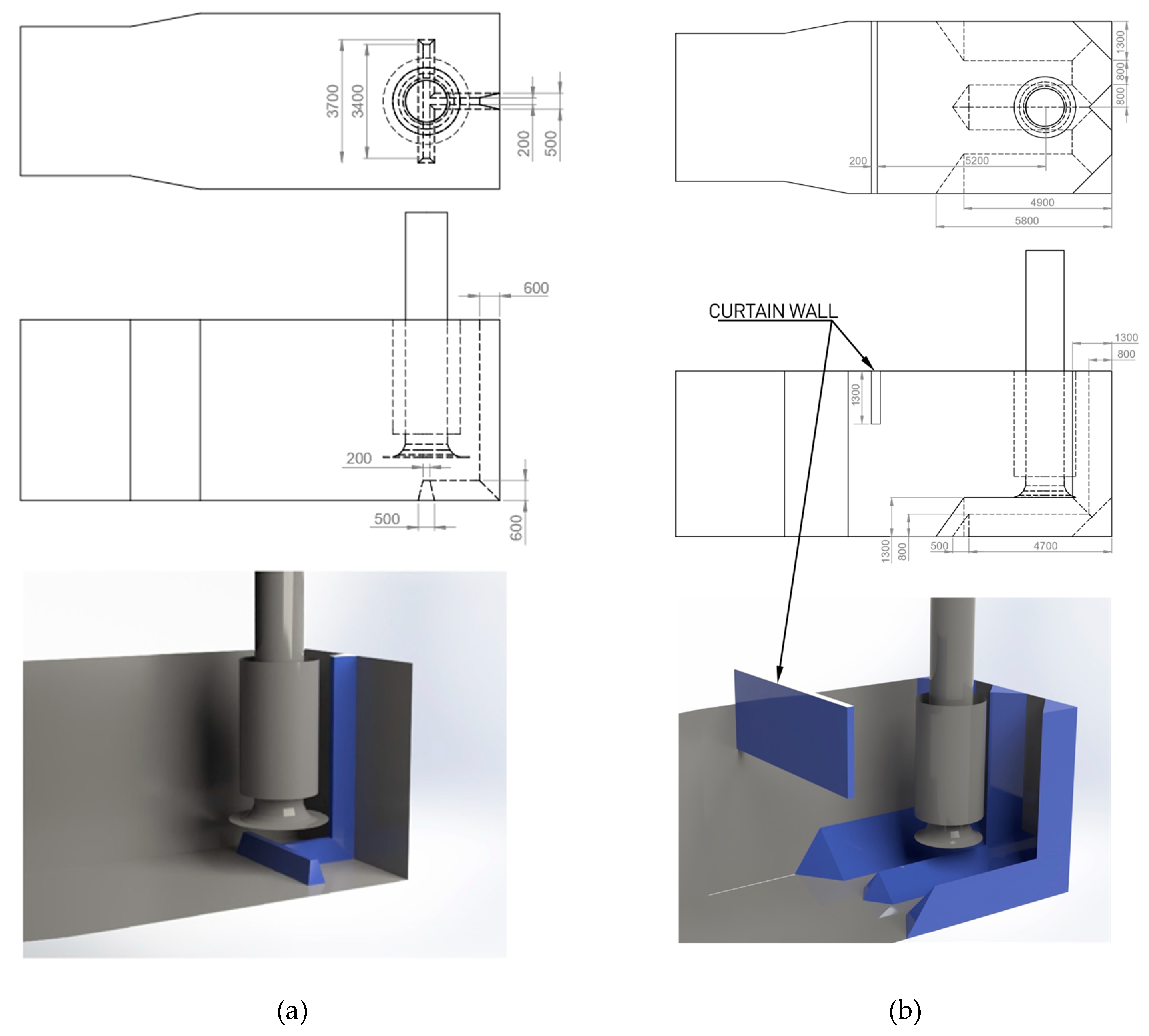
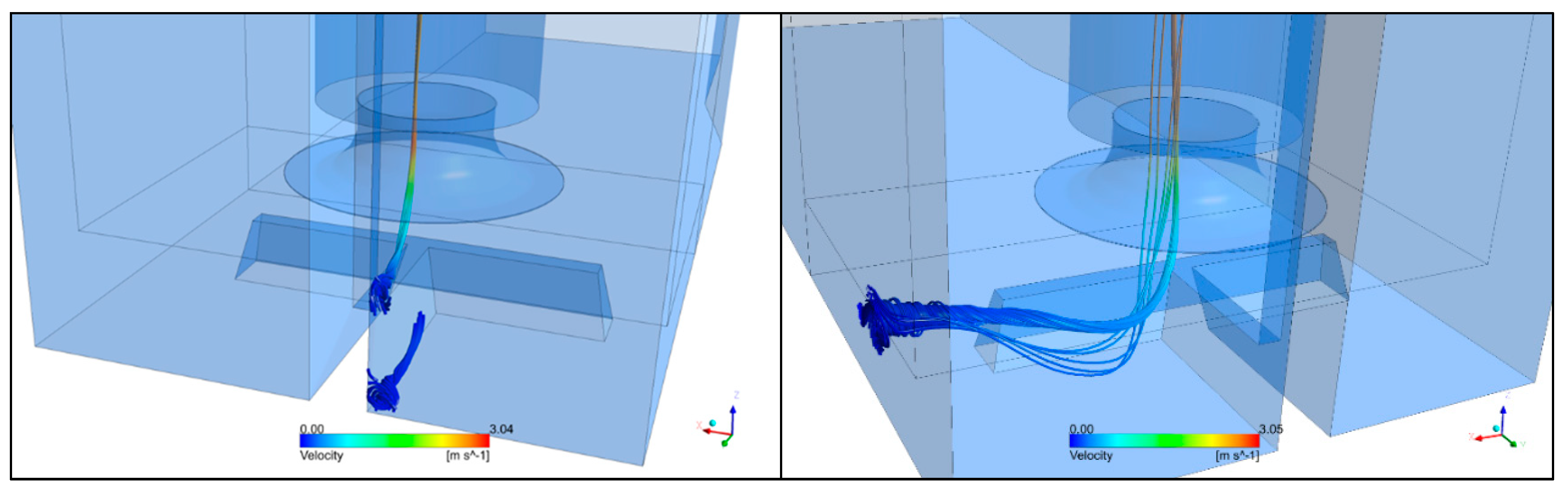
For the model used for the baseline test, the strength of the submerged side wall and floor vortices observed both in the physical model test and CFD simulation rendered the initial design unacceptable as per established performance criteria. However, additional CFD simulation showed that the strong vortices can be successfully suppressed by the installation of a trident-shaped triangular floor baffle and 45° corner fillets.
Based on the comparison of these results, it can be concluded that CFD simulation can serve as a viable means of evaluating sump performance. CFD could provide the necessary insight in the flow performance within pump sump thereby possibly reducing the need for extensive physical experiments.
Lastly, it was observed that CFD could provide results within a shorter period of time with a lower financial impact but the speed at which design revision can be made in CFD compared with the physical model is debatable. CFD design revision often requires new geometries and meshes and various pre-processing steps which are considered as the most time-consuming process. While the physical model test merely requires the installation of dummy geometries (e.g., fillet, splitters, AVDs) during each test iteration. Nevertheless, even at least from a financial perspective, CFD may still be a viable option in developing optimum intake designs.

Author Contributions

Conceptualization, V.M.A.; methodology, V.M.A. and L.A.M.D.; software, V.M.A., B.E.A. and L.A.M.D.; validation, V.M.A. and L.A.M.D.; formal analysis, V.M.A. and L.A.M.D.; investigation, V.M.A.; resources, V.M.A.; data curation, B.E.A., P.L.R., and J.G.T.R.; writing—original draft preparation, V.M.A. and L.A.M.D.; writing—review and editing, B.E.A., P.L.R., and J.G.T.R.; visualization, V.M.A. and L.A.M.D.; supervision, B.E.A., P.L.R., and J.G.T.R., L.A.M.D.; funding acquisition, L.A.M.D. All authors have read and agreed to the published version of the manuscript.

Funding

This research was funded by the Department of Science and Technology (DOST) through the Engineering Research and Development for Technology (ERDT) Program—Local Graduate Scholarships. The APC was funded by DOST-ERDT Faculty Research Dissemination Grant.

Acknowledgments

The authors would like to thank Hitachi Plant Technologies, Ltd. Philippine Branch Office for granting permission to use the pump physical model test data presented as well as the meshing software used in this paper.

Conflicts of Interest

The authors declare no conflict of interest.

References

  1. Knauss, J. Swirling Flow Problems at Intakes; Balkema, A.A., Ed.; International Association for Hydraulic Research: Rotterdam, The Netherlands, 1987. [Google Scholar]
  2. Chang, E. Experimental Data on the Hydraulic Design of Intakes and Pump Sumps; Report RR1518; British Hydromechanics Reseach Association: Bedfordshire, UK, 1979. [Google Scholar]
  3. American National Standard. Pump Intake Design; ANSI/HI 9.8-1998; Hydraulic Institute: Parsippany, NJ, USA, 2012. [Google Scholar]
  4. Pascoa, J.; Mendes, A.; Gato, L. A fast iterative inverse method for turbomachinery blade design. Mech. Res. Commun. 2009, 36, 630–637. [Google Scholar] [CrossRef]
  5. Keck, H.; Weiss, T.; Michler, W.; Sick, M. Recent developments in the dynamic analysis of water turbines. In Proceedings of the 2nd IAHR International Meeting of the Workgroup on Cavitation and Dynamic Problems in Hydraulic Machinery and Systems, Timisoara, Romania, 24–26 October 2007; pp. 9–20. [Google Scholar]
  6. Keck, H.; Sick, M. Thirty years of numerical flow simulation in hydraulic turbomachines. Acta Mech. 2008, 201, 211. [Google Scholar] [CrossRef]
  7. Constantinescu, G.S.; Patel, V.C. Numerical Model for Simulation of Pump-Intake Flow and Vortices. J. Hydraul. Eng. 1998, 124, 123–134. [Google Scholar] [CrossRef]
  8. Rajendran, V.P.; Constantinescu, G.; Patel, V.C. Experimental Validation of Numerical Model of Flow in Pump-Intake Bays. J. Hydraul. Eng. 1999, 125, 1119–1125. [Google Scholar] [CrossRef]
  9. Li, S.; Silva, J.M.; Lai, Y.; Weber, L.J.; Patel, V.C. Three-dimensional simulation of flows in practical water-pump intakes. J. Hydroinformatics 2006, 8, 111–124. [Google Scholar] [CrossRef]
  10. Lai, Y.G.; Weber, L.J.; Patel, V.C. A non-hydrostatic three-dimensional numerical model for hydraulic flow simulation—Part II: Validation and application. J. Hydraul. Eng. 2003, 129, 206–214. [Google Scholar] [CrossRef]
  11. Okamura, T.; Kamemoto, K.; Matsui, J. CFD Prediction and model Experiment on Suction Vortices in pump sump. In Proceedings of the 9th Asian Conference on Fluid Machinery, Jeju, Korea, 16–19 October 2007. [Google Scholar]
  12. Wicklein, E.; Sweeney, C.; Senon, C.; Hattersley, D.; Schultz, B.; Naef, R. Computation Fluid Dynamic Modeling of a Proposed Influent Pump Station. Proc. Water Environ. Fed. 2006, 2006, 7094–7114. [Google Scholar] [CrossRef] [Green Version]
  13. Shukla, S.N.; Kshirsagar, J. Numerical prediction of cavitation in model pump. In Proceedings of the ASME 2008 International Mechanical Engineering Congress and Exposition, Boston, MA, USA, 31 October–6 November 2008. [Google Scholar]
  14. Nagahara, T.; Sato, T.; Kawabata, S.; Okamura, T. Effect of submerged vortex cavitation in pump suction intakes on mixed flow pump impeller. Turbomach. Soc. Jpn. 2002, 30, 70–75. [Google Scholar]
  15. Tang, X.; Wang, F.J.; Li, Y.; Cong, G.H.; Shi, X.Y.; Wu, Y.L.; Qi, L.Y. Numerical investigations of vortex flows and vortex suppression schemes in a large pumping-station sump. Proc. Inst. Mech. Eng. Part C: J. Mech. Eng. Sci. 2011, 225, 1459–1480. [Google Scholar] [CrossRef]
  16. Kanemori, Y.; Pan, Y. Surface vortex prediction and preventing technique in pump intake sump. Turbomachinery 2015, 43, 90–98. (In Japanese) [Google Scholar]
  17. Yamade, Y.; Kato, C.; Nagahara, T.; Matsui, J. Numerical investigations of submerged vortices in a model pump sump by using Large Eddy Simulation. IOP Conf. Series: Earth Environ. Sci. 2016, 49, 32003. [Google Scholar] [CrossRef] [Green Version]
  18. Ohyama, S.; Tsukamoto, H.; Oshikawa, T.; Miyazaki, K.; Ohishi, M. Visualization and numerical analysis of unsteady flow in pump sump. Turbomachinery 2008, 36, 746–755. (In Japanese) [Google Scholar]
  19. Qian, Z.; Wu, P.; Guo, Z.; Huai, W.-X. Numerical simulation of air entrainment and suppression in pump sump. Sci. China Technol. Sci. 2016, 59, 1847–1855. [Google Scholar] [CrossRef]
  20. Ahn, S.-H.; Xiao, Y.; Wang, Z.; Zhou, X.; Luo, Y. Numerical prediction on the effect of free surface vortex on intake flow characteristics for tidal power station. Renew. Energy 2017, 101, 617–628. [Google Scholar] [CrossRef]
  21. Menter, F. Review of the shear-stress transport turbulence model experience from an industrial perspective. Int. J. Comput. Fluid Dyn. 2009, 23, 305–316. [Google Scholar] [CrossRef]
  22. ANSYS, Inc. ANSYS Fluent Theory Guide; ANSYS, Inc.: Canonsburg, PA, USA, 2018. [Google Scholar]
Figure 1. 3D rendering of the 1:10 undistorted scale hydraulic model test.
Energies 13 06136 g001
Figure 2. Pump sump model for numerical analysis.
Energies 13 06136 g002
Figure 3. Overview of the boundary conditions and fluid domains for the numerical analysis.
Energies 13 06136 g003
Figure 4. Cutaway view of the meshed model showing 4 regions with varying mesh densities to reduce calculation time.
Energies 13 06136 g004
Figure 5. CFD Mesh for Grid Independence Study. (a) Coarse Mesh, (b) Medium Mesh, (c) Fine Mesh.
Energies 13 06136 g005
Figure 6. Axial Velocity at Bell Inlet.
Energies 13 06136 g006
Figure 7. Velocity at line parallel to flow.
Energies 13 06136 g007
Figure 8. Injecting dye across the width of the pump bay shows a uniform and stable approach flow.
Energies 13 06136 g008
Figure 9. Flow streamline near the bottom of the sump indicating steady and uniform approach flow towards the pumps.
Energies 13 06136 g009
Figure 10. Strong type 2 floor vortex activity even with a maximum floor clearance of 0.5D (130 mm).
Energies 13 06136 g010
Figure 11. Intermittent side wall vortex. Type 1 to occasional type 3. Combined with the floor vortex increases the swirl along the pump column.
Energies 13 06136 g011
Figure 12. Backwall submerged vortex type 2 to type 3 as evidenced by the solid dye core.
Energies 13 06136 g012
Figure 13. Flow instability and drifting behind the pump.
Energies 13 06136 g013
Figure 14. Image shows a free-surface vortex developing from a type 1 surface dimple (left) to a type 3 full dye core (right) vortex.
Energies 13 06136 g014
Figure 15. (a) strong sub-surface vortex attached to the backwall of the sump. (b) floor vortex as photographed during the physical model test. (c) vector plot showing flow direction near the backwall.
Energies 13 06136 g015
Figure 16. Floor vortex and sidewall vortex.
Energies 13 06136 g016
Figure 17. CFD results showing streamline indicating the presence of a surface vortex.
Energies 13 06136 g017
Figure 18. Proposed fillet-splitter design to reduce vortex formation: (a) trapezoidal-shaped cross floor baffle with vertical backwall splitter; (b) trident-shaped triangular floor baffle and 45° corner fillets.
Energies 13 06136 g018
Figure 19. Sidewall and backwall vortices observed on numerical results.
Energies 13 06136 g019
Figure 20. Vector plot showing uniform flow pattern on the sidewalls and sump floor.
Energies 13 06136 g020
Figure 21. Flow remains attached to the wall and the surface of the splitters. No flow separation observed.
Energies 13 06136 g021
Figure 22. CFD results of swirl angle measurements.
Energies 13 06136 g022
Figure 23. Point velocity profile for the physical model test.
Energies 13 06136 g023
Figure 24. Point velocity taken on points on a plane across the impeller eye (CFD).
Energies 13 06136 g024
Table 1. Calculated Reynolds number and Weber number at the suction bell.
CriteriaValueMinimumAcceptable
R e 1.44 × 10 5 6 × 10 4 ok
W e 1.37 × 10 3 240 ok
Table 2. Flow parameters for the physical model.
ParameterValue
Flow rate (m3/h)116
Suction Bell Diameter (mm)260
Bellmouth Throat Diameter (mm)125.7
Bellmouth Submergence (mm)418.4
Floor Clearance (mm)130
Table 3. Maximum short-term and average long-term swirl angles for the physical model test.
Rotation DirectionClockwiseCounterclockwise
Max. short-term pre-rotation (rounds per 30 s)206
Short term swirl angle7.5°
  • % time swirl is above 5°
86.7%
  • % time swirl is above 7°
68.4%
Ave long-term pre-rotation (per 900 s)94
Long term swirl angle1.88°
Model Flow = 116.07 m3/h, D i = 0.1257 m.
Publisher’s Note: MDPI stays neutral with regard to jurisdictional claims in published maps and institutional affiliations.

