An Optimal Phase Arrangement of Distribution Transformers under Risk Assessment


Abstract
:1. Introduction
2. Problem Description
2.1. Power Balance
2.2. Voltage Constraints
2.3. The Unbalance Factor Constraints
3. Solution Algorithm
3.1. Generation VAR of WTs/PVs
3.2. Feasible Particle Swarm Optimization (FPSO)
3.3. Implementation of Searching Procedure
- (a)
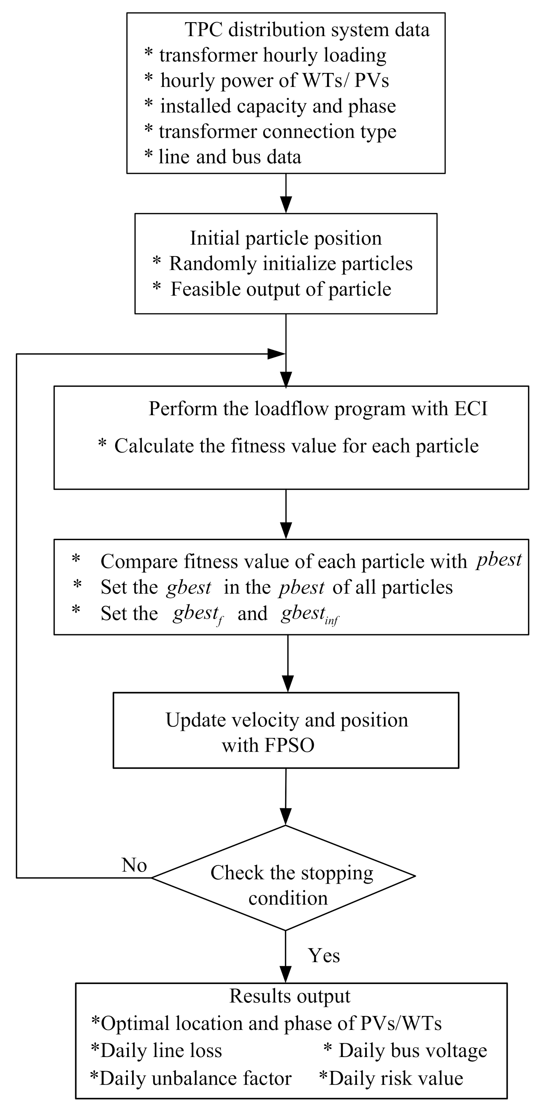
- Calculate the transformer hourly loading in a TPC distribution feeder.
- (b)
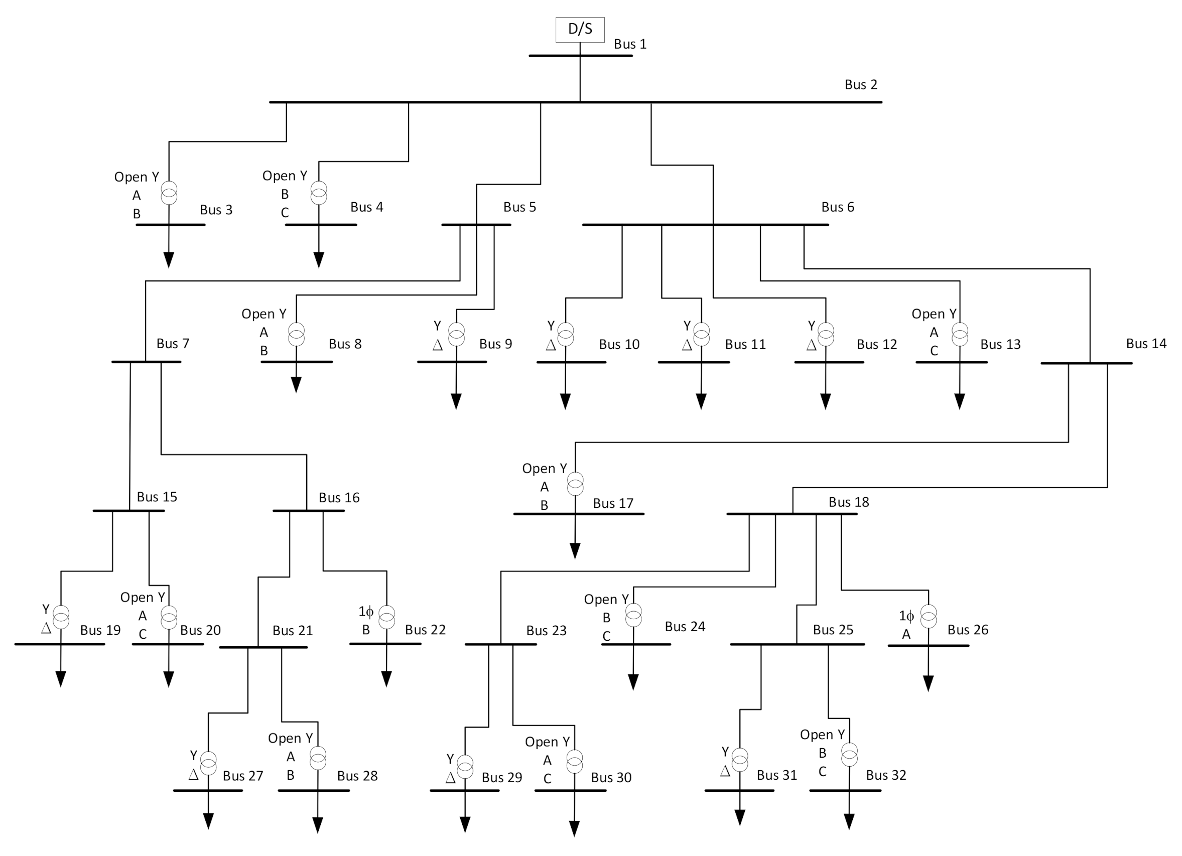
- Input the line data and bus data of the TPC distribution feeder. The bus data has the loads, types and phase of the distribution transformers, the number of WTs/PVs, and the generation VAR of the WTs/PVs.
- (c)
- Randomly initialize 30 particles with feasible connection of distribution transformers, and the phase and location of WTs/PVs.
- (d)
- Perform the load flow program with ECI and calculate the fitness values of each particle in the 24-hour interval. The fitness function is defined in Equation (13).
- (e)
- Compare each particle’s fitness value with the . If the objective value is smaller than the , set the value as the current .
- (f)
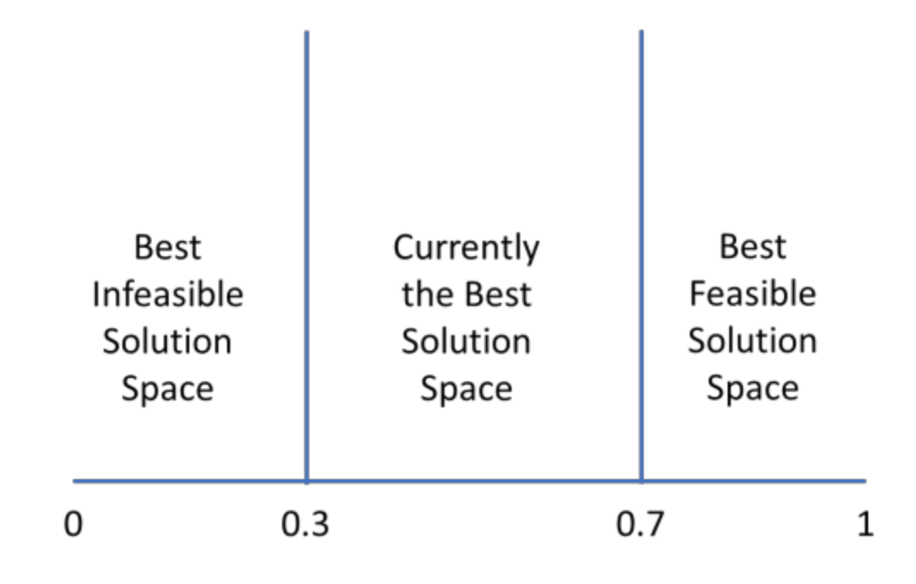
- If the penalty factor is equal to 0 (), the best particle associated with the minimal of all particles is set to the value of this as the current .
- (g)
- If the penalty factor is more than 0 (), the best particle is set to .
- (h)
- Perform the FPSO according to Equation (22) for each particle and update velocity and position vectors.
- (i)
- The stopping condition is 100 generations. If the preset stopping condition is not yet reached, then go back to Step (d).
4. Case Study
4.1. The Optimal Location of WTs and PVs
4.2. The Optimal Phase Connection of the Transformers
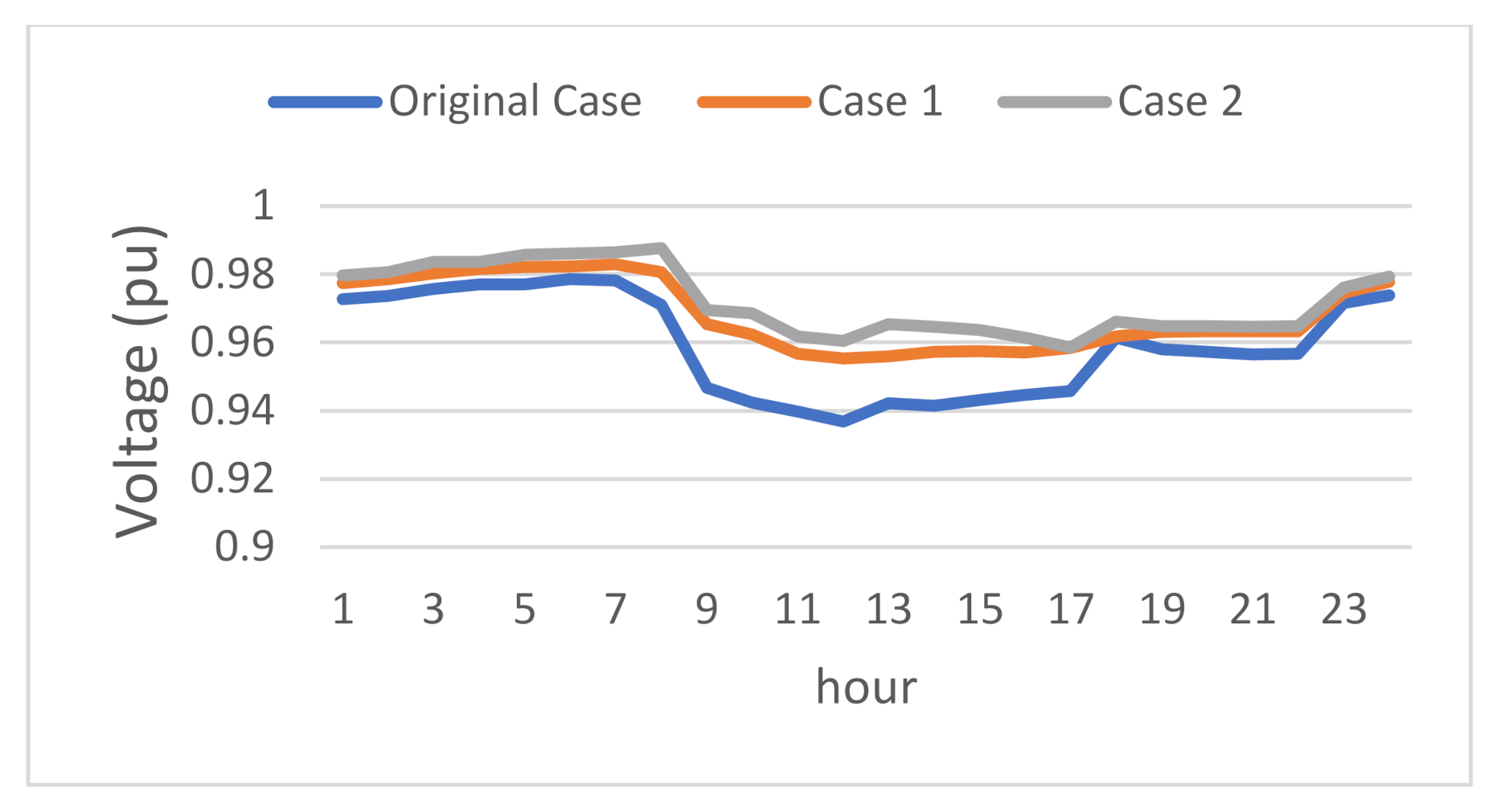
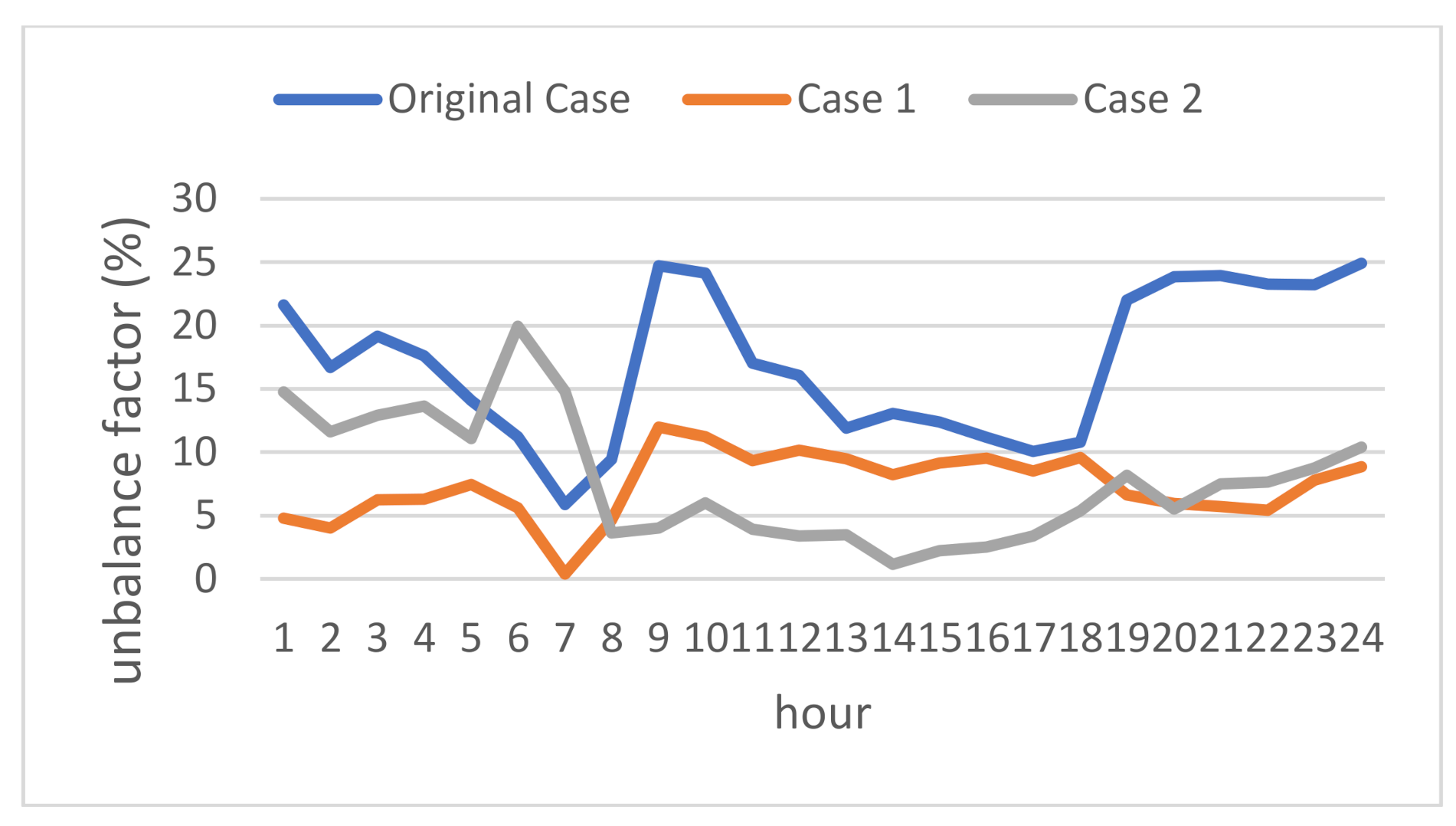
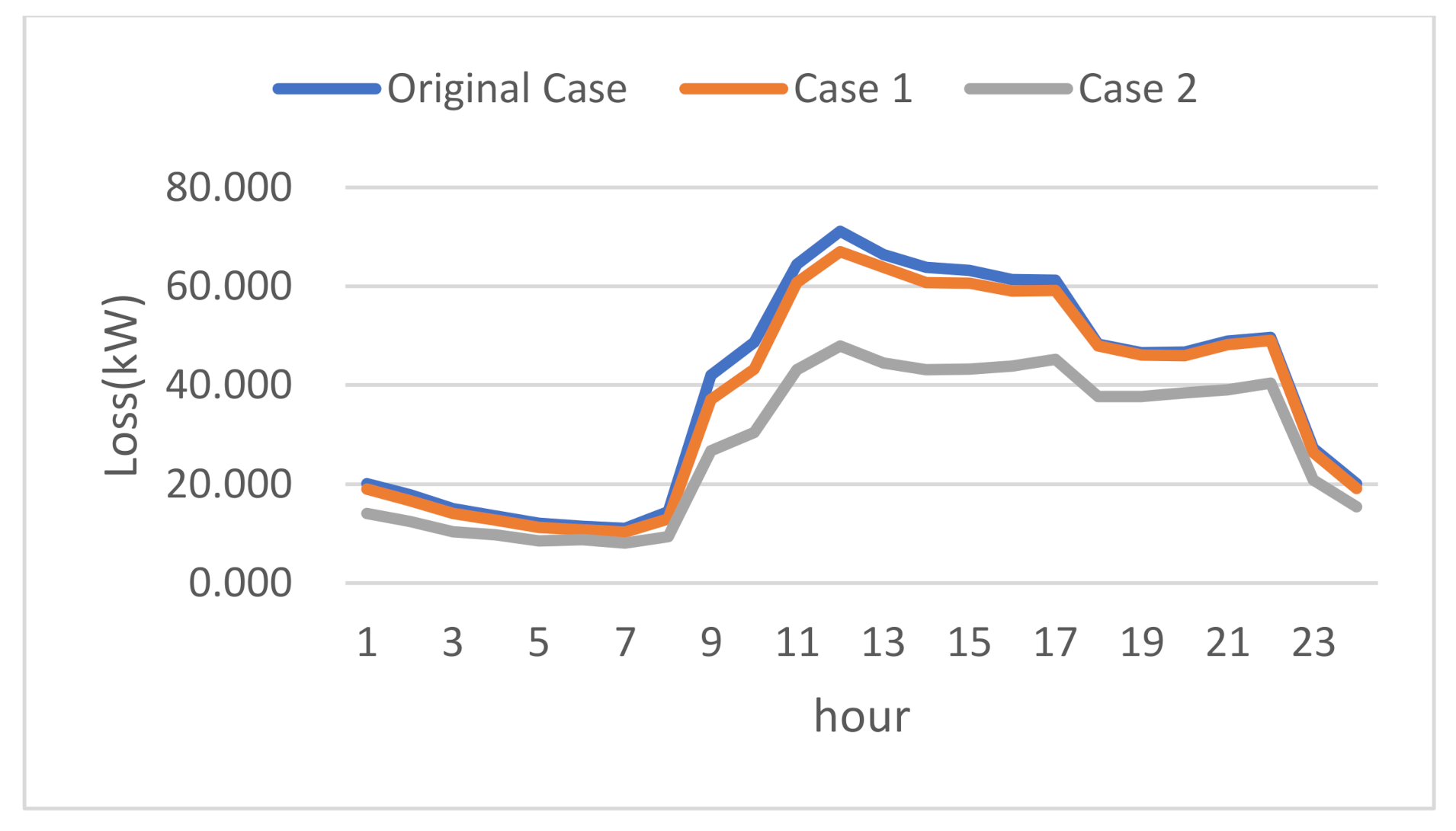
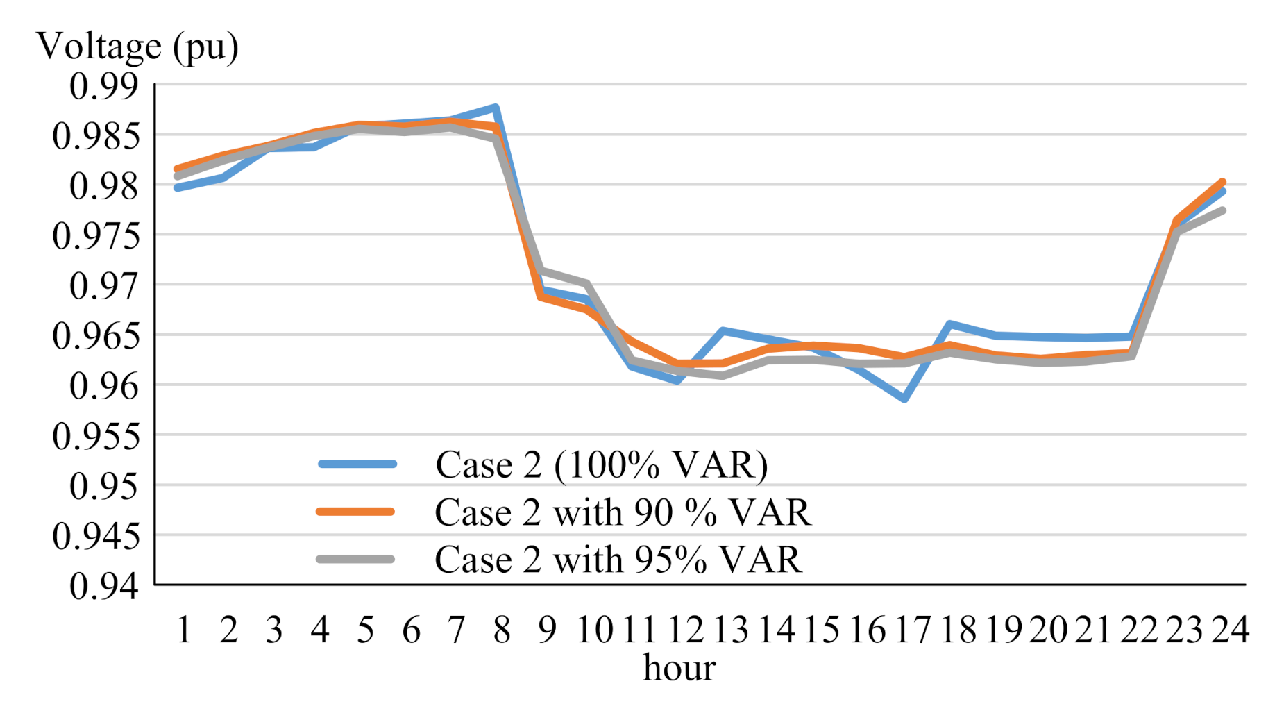
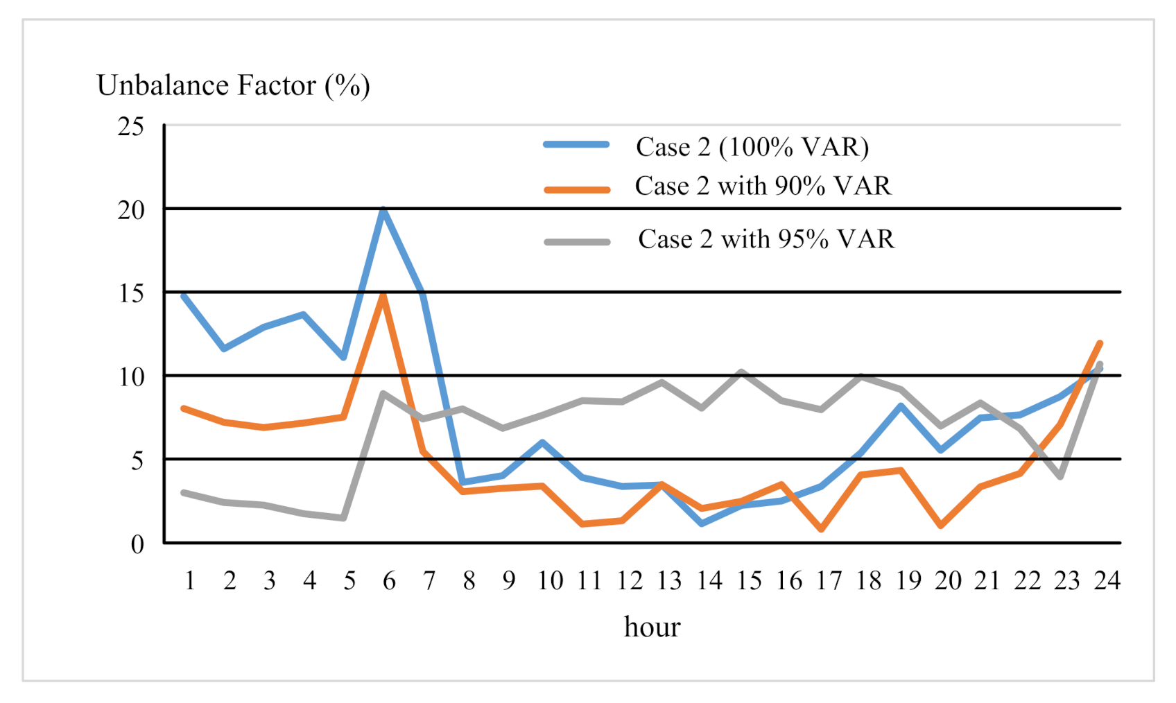
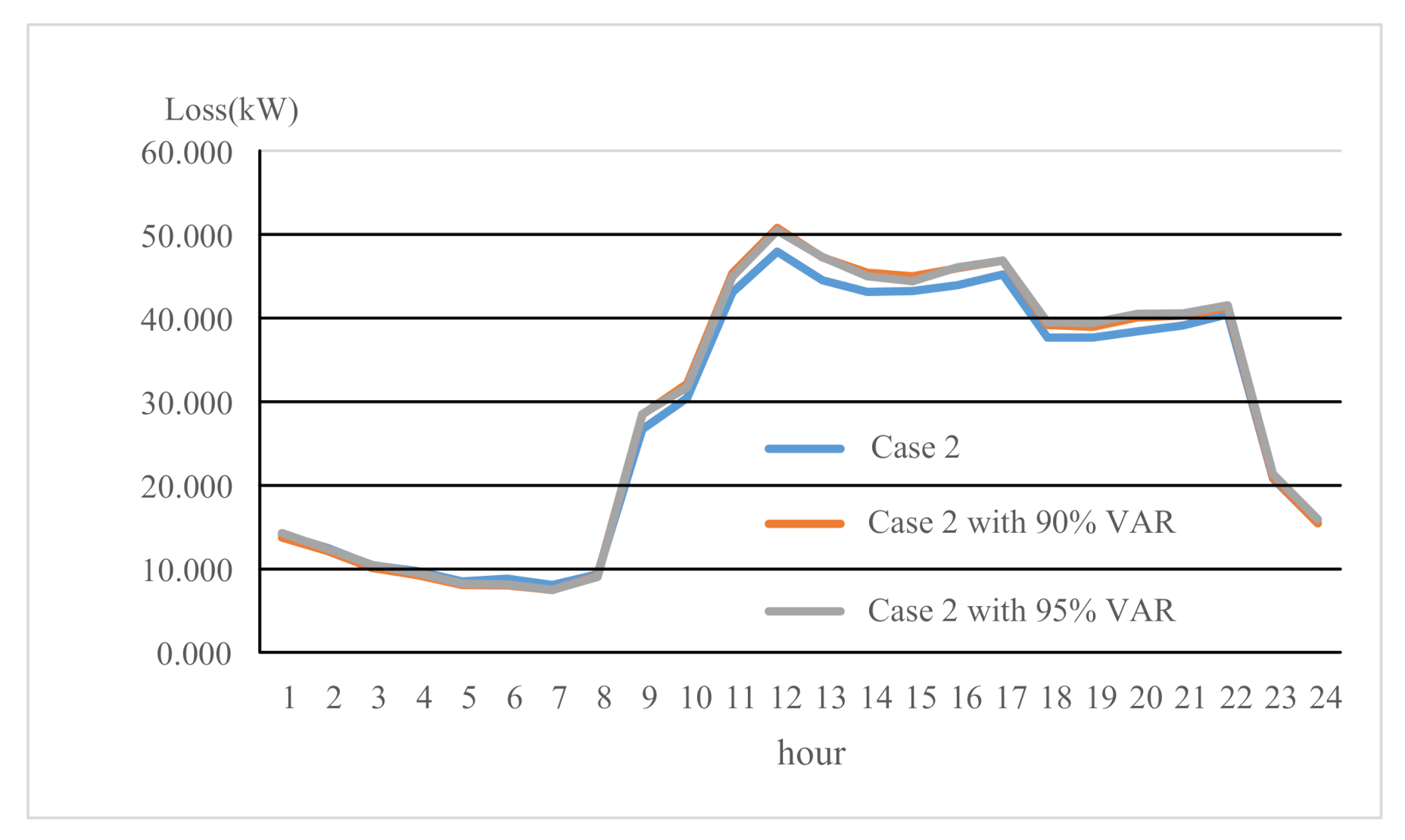
4.3. The Optimal Phase Connection of the Transformers Considering the Generation of WTs/PVs
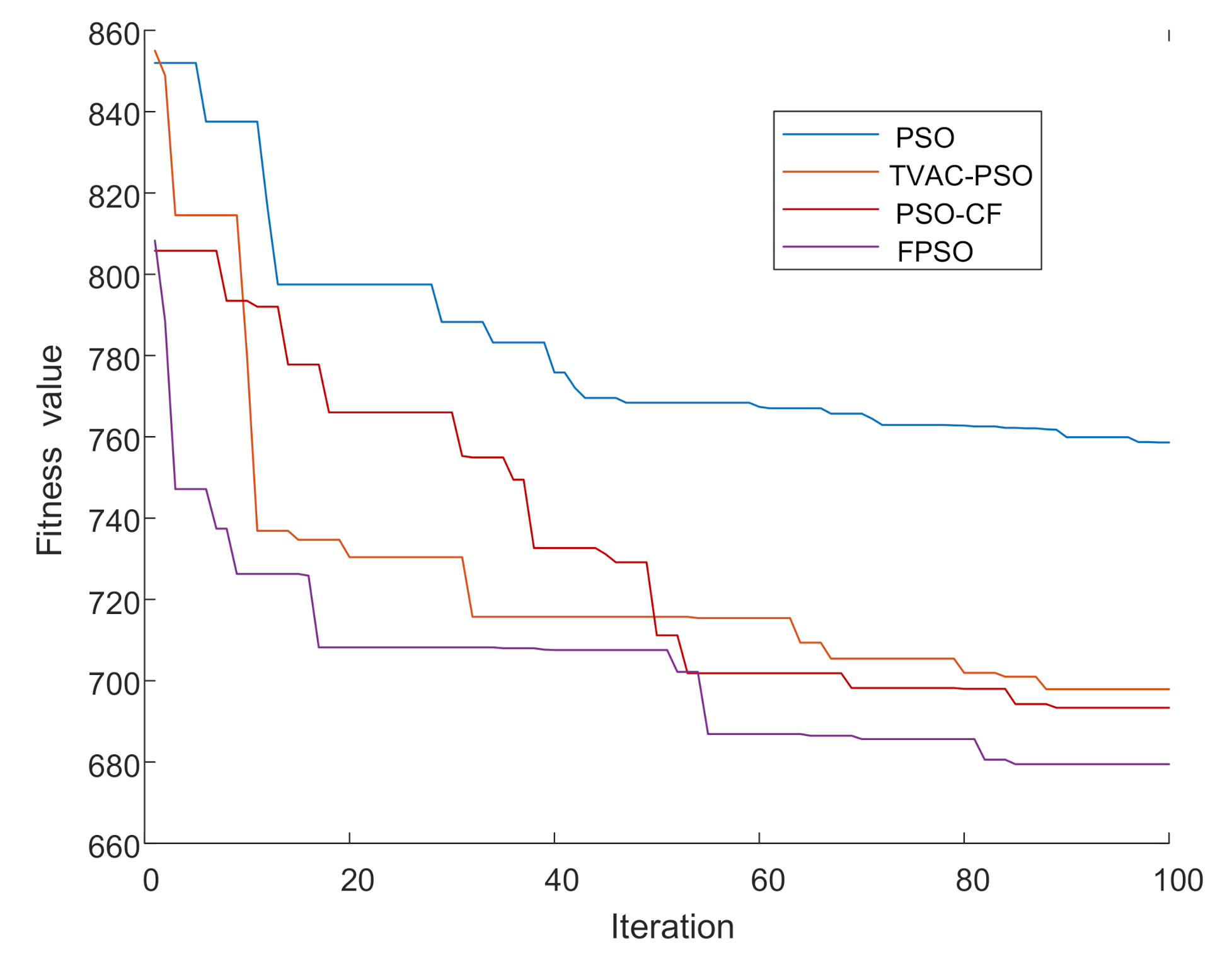
4.4. Convergence Test
5. Conclusions
Author Contributions
Funding
Acknowledgments
Conflicts of Interest
Abbreviations
| Symbols | Abbreviations |
| air density () | |
| the rotor area ( | |
| the speed of WT ( at time | |
| the VAR of wind speed ( at time | |
| the ratio of tip speed | |
| the pitch angle of rotor blades (deg.) | |
| the global radiation () at time | |
| the PV array area () | |
| the operating efficiency of PV | |
| the VAR of global radiation ()at time | |
| acceleration constant | |
| uniformly distributed random variables between 0 and 1 | |
| the position of particle at iteration | |
| the velocity of particle at iteration | |
| the own best position of particle at iteration | |
| the best particle in the swarm at iteration | |
| the inertia weight at iteration . and |
References
- Chang, C.Y.; Yu, J.S.; Chen, C.S. Effects of open-wye/open-delta transformers on the operation of distribution systems. Electr. Power Syst. Res. 1986, 10, 1671–1674. [Google Scholar] [CrossRef]
- Huang, S.J.; Tai, T.Y.; Liu, X.Z.; Su, W.F.; Gu, P.H. Application of bird-mating optimization to phase adjustment of open-wye/open-delta transformers in a power grid. In Proceedings of the IEEE International Conference on Industrial Technology (ICIT), Seville, Spain, 17–19 March 2015; Volume 1, pp. 12279–12751. [Google Scholar]
- Chin, H.C.; Chung, R.J.; Yu, J.S.; Sun, H.H. Application of the ant colony system for open wye-open delta transformer’s phase sequence adjustment. In Proceedings of the IEEE Region 10 TENCON 2004 Conference, Chiang Mai, Thailand, 21–24 November 2004; pp. 432–435. [Google Scholar]
- Adefarati, T.; Bansal, R.C. Integration of renewable distributed generators into the distribution system: A review. IET Renew. Power Gener. 2016, 10, 8738–8784. [Google Scholar] [CrossRef]
- Mahmud, K.; Khan, B.; Ravishankar, J.; Ahmadi, A.; Siano, P. An internet of energy framework with distributed energy resources, prosumers and small-scale virtual power plants: An overview. Renew. Sustain. Energy Rev. 2020, 127, 109840. [Google Scholar] [CrossRef]
- Yuen, R.; Stoev, S.; Cooley, D. Distributionally robust inference for extreme Value-at-Risk. Insur. Math. Econ. 2020, 92, 708–709. [Google Scholar] [CrossRef] [Green Version]
- Pérez, O.R.; Watts, D.; Flores, Y. Planning in a changing environment: Applications of portfolio optimisation to deal with risk in the electricity sector. Renew. Sustain. Energy Rev. 2018, 82, 38083–38823. [Google Scholar] [CrossRef]
- Chen, T.H.; Cherng, J.T. Optimal phase arrangement of distribution transformers connected to a primary feeder for system unbalance improvement and loss reduction using a Genetic algorithm. IEEE Trans. Power Syst. 2000, 15, 9941. [Google Scholar]
- Su, Y.S.; Lin, W.M.; Chang, S.C.; Tsay, M.T. Application of the normalized weighting method for the connections between distribution transformers and a primary feeder. In Proceedings of the 2004 IEEE Region 10 Conference TENCON, Chiang Mai, Thailand, 24–24 November 2004; pp. 4451–4484. [Google Scholar]
- Abril, I.P. NSGA-II phase balancing of primary distribution circuits by the reconnection of their circuit laterals and distribution transformers. Electr. Power Syst. Res. 2014, 109, 1–7. [Google Scholar] [CrossRef]
- Abril, I.P. Genetic algorithm for the load balance on primary distribution circuit. IEEE Lat. Trans. 2010, 8, 5231–5265. [Google Scholar] [CrossRef]
- Singh, D.; Misra, R.K.; Mishra, S. Distribution system feeder re-phasing considering voltage-dependency of loads. Int. J. Electr. Power Energy Syst. 2016, 76, 1071–1109. [Google Scholar] [CrossRef]
- Ali, B.; Siddique, I. Distribution system loss reduction by automatic transformer load balancing. In Proceedings of the International Multi-topic Conference (INMIC), Lahore, Pakistan, 24–26 November 2017; Volume 1, pp. 1–5. [Google Scholar]
- Kuo, C.C. Application of the normalized weighting method for the connections between distribution transformers and a primary feeder. In Proceedings of the 39th International Universities Power Engineering Conference, Bristol, UK, 6–8 September 2004; Volume 1, pp. 343–348. [Google Scholar]
- Tsay, M.T.; Chan, S.Y. The optimal loss reduction of distribution feeder based on transformer rearrangement. Int. J. Electr. Power Energy Syst. 2001, 23, 3433–3448. [Google Scholar] [CrossRef]
- Tsay, M.T.; Chan, S.Y. Improvement in system unbalance and loss reduction of distribution feeders using transformer phase rearrangement and load diversity. Int. J. Electr. Energy Energy Syst. 2003, 25, 3901–3954. [Google Scholar] [CrossRef]
- Maria, T.C.C.; Daniel, D.A.; Elisa, T.B. Locational impact and network costs of energy transition: Introducing geographical price signals for new renewable capacity. Energy Policy 2020, 141, 111469. [Google Scholar] [CrossRef]
- Chang, C.T. Multi-choice goal programming model for the optimal location of renewable energy facilities Renewable and Sustainable. Energy Rev. 2015, 41, 3789–3793. [Google Scholar]
- Reyes, A.; Sucar, L.E.; Lbargüengoytia, P.H.; Morales, E.F. Planning under uncertainty applications in power plants using factored markov decision processes. Energies 2020, 13, 2302. [Google Scholar] [CrossRef]
- Acebrón, J.A.; Herrero, J.R.; Monteiro, J. A highly parallel algorithm for computing the action of a matrix exponential on a vector based on a multilevel Monte Carlo method. Comput. Math. Appl. 2020, 79, 34515–34953. [Google Scholar] [CrossRef] [Green Version]
- Lin, W.M.; Teng, J.H. Three-phase distribution network fast-decoupled power flow solutions. Int. J. Electr. Power Energy Syst. 2000, 22, 3753–3780. [Google Scholar] [CrossRef]
- Alexander, C. Risk Management and Analysis—Volume 1 Measuring and Modelling Financial Risk; John Wiley & Sons Ltd.: Hoboken, NJ, USA, 2000. [Google Scholar]
- Marrison, C. Fundamentals of Risk Measurement; McGraw-Hill Companies, Inc.: New York, NY, USA, 2002. [Google Scholar]
- Mastsumoto, M.; Ohori, R.; Yoshiki, T. Approximation of Quasi-Monte Carlo worst case error in weighted spaces of infinitely times smooth functions. J. Comput. Appl. Math. 2018, 33, 1551–1564. [Google Scholar]
- Kennedy, J.; Eberhart, R.C. Particle Swarm Optimization. In Proceedings of the IEEE International Conference on Neural Networks, Perth, Australia, 27 November–1 December 1995; Volume 4, pp. 19421–19948. [Google Scholar]
- Chaturvedi, K.T.; Pandit, M.; Srivastava, I. Self-organizing hierarchical particle swarm optimization for nonvex economic dispatch. IEEE Trans. Power Syst. 2008, 23, 10798–107987. [Google Scholar] [CrossRef]
- Chang, S.C. Transformer Load Connection and Loss Reduction for Distribution Feeder Circuits. Master’s Thesis, National Sun Yat-Sen University, Kaohsiung City, Taiwan, 1997. [Google Scholar]
- Rituraj, S.P.; Nitin, N.; Harish, G. A novel TVAC-PSO based mutation strategies algorithm for generation scheduling pumped storage hydrothermal system incorporating solar units. Energy 2018, 142, 8228–8237. [Google Scholar]
- Shi, Y.; Eberhart, R.C. A Modified Particle Swarm Optimizer. In Proceedings of the IEEE International Conference on Evolutionary Computation, Anchorage, AK, USA, 4–9 May 1998; pp. 693–697. [Google Scholar]
- Central Weather Bureau Observation Taiwan. 2020. Available online: https://www.cwb.gov.tw/V7/observe/ (accessed on 1 March 2020).


| Type | Transformer | Open-Wye/Open-Delta Transformer | Single-Phase Transformer | ||||||
|---|---|---|---|---|---|---|---|---|---|
| 1 | A | B | C | A | B | x | A | x | x |
| 2 | A | C | B | A | x | C | x | B | x |
| 3 | B | A | C | x | B | C | x | x | C |
| 4 | B | C | A | - | - | - | - | - | - |
| 5 | C | A | B | - | - | - | - | - | - |
| 6 | C | B | A | - | - | - | - | - | - |
| Load | Load | Load | Load | ||||||||
|---|---|---|---|---|---|---|---|---|---|---|---|
| 1 | − | − | 9 | Y−Δ | A, B, C | 17 | Open Y | A, B | 25 | − | − |
| 2 | − | − | 10 | Y−Δ | A, B, C | 18 | − | − | 26 | 1 | A |
| 3 | Open Y | A, B | 11 | Y−Δ | A, B, C | 19 | Y−Δ | A, B, C | 27 | Y−Δ | A, B, C |
| 4 | Open Y | B, C | 12 | Y−Δ | A, B, C | 20 | Open Y | A, C | 28 | Open Y | A, B |
| 5 | − | − | 13 | Open Y | A, C | 21 | − | − | 29 | Y−Δ | A, B, C |
| 6 | − | − | 14 | − | − | 22 | 1 | B | 30 | Open Y | A, C |
| 7 | − | − | 15 | − | − | 23 | − | − | 31 | Y−Δ | A, B, C |
| 8 | Open Y | A, B | 16 | − | − | 24 | Open Y | B, C | 32 | Open Y | B, C |
| Optimal Location | Location 90% VAR | Location 95%VAR | ||||
|---|---|---|---|---|---|---|
| WT1 | 19 | 1 | 19 | 1 | 18 | 3 |
| WT2 | 20 | 3 | 20 | 3 | 20 | 1 |
| PV1 | 17 | 3 | 17 | 3 | 18 | 1 |
| PV2 | 20 | 3 | 20 | 3 | 19 | 1 |
| Bus No. | Transformer Type | Original Connected | Phase Rearrangement | Phase Rearrangement with 90% VAR | Phase Rearrangement with 95%VAR |
|---|---|---|---|---|---|
| 3 | A, B | A, B | A, B | A to C, B | |
| 4 | B, C | B, C | B, C | B, C | |
| 8 | A, B | A to C, B | A to C, B | A to C, B | |
| 9 | A, B, C | A to C, B, C to A | A to C, B, C to A | A to C, B, C to A | |
| 10 | A, B, C | A, B, C | A, B, C | A, B, C | |
| 11 | A, B, C | A to C, B, C to A | A to C, B, C to A | A to C, B, C to A | |
| 12 | A, B, C | A, B, C | A, B, C | A, B, C | |
| 13 | A, C | A to C, C to A | A to C, C to A | A to C, C to A | |
| 17 | A, B | A, B | A, B | A, B | |
| 19 | A, B, C | A to C, B, C to A | A to C, B, C to A | A to C, B, C to A | |
| 20 | A, C | A to C, C to A | A to C, C to A | A to C, C to A | |
| 22 | B | B | B | B | |
| 24 | B, C | B, C to A | B, C to A | B, C to A | |
| 26 | A | A to C | A to C | A to C | |
| 27 | A, B, C | A to C, B to A, C to B | A to C, B to A, C to B | A to C, B, C to A | |
| 28 | A, B | A, B to C, | A, B to C | A to B, B to C | |
| 29 | A, B, C | A to B, B to C, C to A | A to B, B to C | A, B, C | |
| 30 | A, C | A, C | A, C | A, C | |
| 31 | A, B, C | A to C, B, C to A | A to C, B, C to A | A to C, B, C to A | |
| 32 | B, C | B, C | B, C | B, C to A |
| PSO | TVAC-PSO | PSO-CF | FPSO | |
|---|---|---|---|---|
| Max. Convergent Fitness Value | 959.098 | 927.018 | 897.813 | 861.843 |
| Min. Convergent Fitness Value | 758.617 | 697.927 | 693.345 | 679.459 |
| Average Convergent Fitness Value | 826.085 | 781.681 | 768.916 | 744.558 |
| CPU Time (sec) | 48.67 | 56.184 | 83.731 | 60.821 |
Publisher’s Note: MDPI stays neutral with regard to jurisdictional claims in published maps and institutional affiliations. |
© 2020 by the authors. Licensee MDPI, Basel, Switzerland. This article is an open access article distributed under the terms and conditions of the Creative Commons Attribution (CC BY) license (http://creativecommons.org/licenses/by/4.0/).
Share and Cite
Tu, C.-S.; Yang, C.-Y.; Tsai, M.-T. An Optimal Phase Arrangement of Distribution Transformers under Risk Assessment. Energies 2020, 13, 5852. https://doi.org/10.3390/en13215852
Tu C-S, Yang C-Y, Tsai M-T. An Optimal Phase Arrangement of Distribution Transformers under Risk Assessment. Energies. 2020; 13(21):5852. https://doi.org/10.3390/en13215852
Chicago/Turabian StyleTu, Chia-Sheng, Chung-Yuen Yang, and Ming-Tang Tsai. 2020. "An Optimal Phase Arrangement of Distribution Transformers under Risk Assessment" Energies 13, no. 21: 5852. https://doi.org/10.3390/en13215852