Catchment Based Aerodynamic Performance Analysis of Small Wind Turbine Using a Single Blade Concept for a Low Cost of Energy

Abstract

For low and medium wind conditions, there is a possibility to harness maximum wind potential reducing the cost of energy by employing catchment-based wind turbine designs. This paper aims to study catchment-based small wind turbine aerodynamic performance for improved efficiency and reduced cost of energy. Hence, design parameters are considered based on specific conditions within a catchment area. The bins and statistical methods implemented with Weibull distribution of wind data for selected sites to characterize the wind conditions and a weighted average method proposed to create representative wind conditions implementing a single blade concept. The blade element method was applied using Matlab code (version R2017a, MathWorks Inc., Natick, MA, US) for aerodynamic design and analysis, and computational fluid dynamics employed using ANSYS—Fluent (version 18.1, ANSYS Inc., Canonsburg, PA, USA) for validation. The performance of the designed blade is evaluated based on annual energy production, capacity factor and power coefficient. Then, for site-specific wind conditions, yearly energy production, and relative cost of energy are examined against rated power. Appropriate rated power for a low cost of energy identified and performance measures evaluated for each site. As a result, a maximum power coefficient of around 51.8% achieved at a design wind speed of 10 m/s, and higher capacity factors of 28% and 50.9% respectively attained for the low and high wind conditions at the proposed rated powers. Therefore, for different wind condition sites, enhanced performance at a low cost of energy could be achieved using a single blade concept at properly selected rated powers employing suitable design conditions and procedures.

1. Introduction

With a growing installation of high wind speed turbines globally, low and medium wind speed turbines are getting more attention [1]. For low and medium wind speed conditions, specific wind turbines shall be designed to utilize the maximum possible wind potential of the site, to reduce loading and costs of energy [2]. Fuglsang et al. showed the potential for a site-specific design that design loads and annual energy production depend on-site with considerably large maximum variations comparing two typical wind turbines at representative wind conditions. The study showed that site-specific turbines generated a smaller cost of energy than a fixed design turbine in every wind climate and appeared to offer great benefits for low-wind-speed sites. In addition to this, the study indicated that the redesign of only blades and towers results in significant reductions in the cost of energy and recommends designing particular wind turbines for low wind speed situations [2]. Regardless of these, it is unmanageable to retain the standard rated-power of any wind turbine at its standard rated value at nonstandard air densities. Hence, to be used for nonstandard sites, it will require adapting to change the standard generator or using extenders with limitations [3]. The cost of energy could also be minimized for onshore and offshore conditions, using a site-specific single wind turbine concept [4].

On top of these, considering the cost of energy, site-specific wind turbine selection was also developed assuming the cost of energy model in terms of the radius of the rotor, hub height, and rated power as variables [5]. For a fixed radius and hub height, the cost of energy increases with rated-power. On the other hand, a variation of lifetime cost could be estimated, in terms of changes in power rating with the assumption of an element of the cost fraction data that vary with changes of rated power [6].

Numerical analysis methods for performance prediction shall be employed to design site-specific wind turbine blades. Computational fluid dynamics (CFD) and the blade element method (BEM) are commonly used numerical analysis tools for wind turbines. BEM is the most frequently used and computationally cheaper tool for designing and investigating the performance of wind turbine blades [7,8,9]. CFD can be used to simulate the aerodynamic characteristics of wind turbine blades and examine the fluid-flows based on the Navier–Stokes equations [9]. In solving the flow fields, Reynolds-averaged Navier–Stokes (RANS) equation is investigated mostly with two-equation turbulence models of the k-ε and k-ω series and four-equation transition k-ω SST (shear stress transport) turbulence model. The k-ε turbulence model is suitable for far-field flow simulations, while the k-ω turbulence model is appropriate in modeling the boundary layers. The transition k-ω SST turbulence model implements the k-ε model for far-field flows and k-ω model for boundary layers. It has mainly been used for the aerodynamic investigation of 3D wind turbine blades and confirmed with experimental results [9,10,11].

Then, it is important to consider the performance measures to evaluate the aerodynamics of the blade. Among the different performance measures of wind turbines, power coefficient (CP), capacity factor (CF), and annual energy production (AEP) are the most common parameters. A review of the performance of small and large turbines shows that a power coefficient of approximately 25% and 45% respectively are depicted [12]. Moreover, typical capacity factors are 20–40% with the values at the higher end of the range in mainly high wind sites [13]. Capacity factors of 35–45% and 20–35% respectively of large and small wind turbines are also depicted [14]. Several parameters affect the capacity factor of wind turbines, which include the generator size and inconsistency of the wind at the site. An inexpensive smaller generator would attain a higher capacity factor and produce a smaller amount of power in high wind speeds. On the contrary, a costly, big generator, which might stall out at low wind speed, would generate slight additional power [15]. The simplified control mechanism and power characteristics of the turbine are also the main reasons for the low capacity factors of small wind turbines [14].

On the other hand, as per the Danish wind industry association, having technically higher efficiency should not be an aim in itself for a wind turbine [16]. With no need to save the free wind, what should matter is the cost of power production out of the winds during the lifetime of the turbine. Therefore, a turbine with the highest yearly energy production is not essentially an optimal one. Capturing a littlepower at higher wind speeds, a combination of a small generator with a large wind turbine could be harnessing power during several hours of the year. On the other hand, demanding a higher starting wind speed, higher efficiency at high wind speeds could be achieved [16].

Therefore, attention should be given to the power density of the wind and wind speed distribution to fix the perfect arrangement of the size of the generator and turbine at various wind sites [16]. Firstly, wind data of the sites should be reviewed in the design processes. Most of the potential methods of reviewing wind data of a particular site use direct or statistical techniques to assess the potential of the wind resource. Among these, the bins method, statistical analysis, development of velocity and power curves from data, and the direct use of averaged data are the most commonly used ones [8].

On the other hand, controllers that can track maximum power are commonly used to ensure maximum energy yield and safety of the wind turbine. A review of the available maximum power point tracking algorithms shows that there are different options to consider depending on the parameters to control. These are tip speed ratio, optimal torque, power signal feedback, and perturbation and observation controls [17]. Along with, for monitoring and maintenance purposes, the state of the wind turbine can be predicted using sensor measurements with repeat-accumulate coded communication methods remotely [18]. A method of a particle filter, which is a nonlinear state estimator, can also be used to estimate the wind turbine parameters like rotor speed, tower top velocity, and tower top displacement [19] to enhance the reliability of the wind turbines.

Even though a lot is done, on the aerodynamic design and analysis of small wind turbines, focusing on the power performance, site-specific conditions, the cost of energy, and related issues do not get due attention. Hence, considering these issues in the design and analysis process are expected to enhance the performance and reduce associated costs. Besides, for off-grid application with one or few installed turbines per site, designing and producing different wind turbine blades is costly for the reason that design and mold making costs are highly expensive when utilizing different blades than a single blade. On the other hand, for sites with various wind conditions, using a single blade at the design rated power might result in a higher cost of energy and low capacity factor than better possible ones.

Thus, the paper considers a single blade concept for use in all the sites in the catchment area. The bins and statistical methods are employed to the wind data of selected sites to characterize the wind condition.A proposed weighted average method is applied to create representative wind characteristics for designing the aerodynamics of the blade using a single blade concept. Catchment-based horizontal-axis wind turbine aerodynamics is analyzed implementing BEM using Matlab code validating it with CFD using Ansys-Fluent. The performance of the designed blade is evaluated based on the annual energy production, capacity factor, and power coefficient applying a maximum power point tracking mechanism. In the end, it examines the relationships between yearly energy production and rated power in terms of the site-specific wind conditions. It also assesses the performance of the blade at each site with the single blade concept and recommending rated-powers for a low cost of energy.

2. Materials and Methods

2.1. Study Area and Wind Data Sites

A study on wind energy resource potential shows that Ethiopia has total wind energy reserves of 3030 GW with exploitable potential of 1599 GW and installable potential of 1350 GW [20,21]. The sites considered in this paper are in the northern part of Ethiopia called Geba catchment located in the surrounding of the city of Mekelle, found at a latitude of 13.48° N, 39.49° E, and around 2208 m elevation. Wind data has been recorded at four wind measurement sites around Mekelle for at least two years. The summary of the selected study sites in the Geba catchment is as shown in

Table 1. Summary of wind measurement sites in Geba catchment.

Wind Measuring Sites	Wind Mast Location Latitude Longitude		Altitude (m)	Height (a.g.l; m)	Available Data Records
					From	To
Dera	13.99° N	39.79° E	2870	30, 10	01/01/2011	31/12/2012
Hagereselam	13.66° N	39.19° E	2628	30, 10	01/01/2011	31/12/2012
Mayderhu	13.29° N	39.40° E	2512	30, 10	01/01/2011	31/12/2012
Mekelle	13.48° N	39.49° E	2208	10, 25	01/01/2011 13/05/2019	31/12/2012 31/05/2020

.

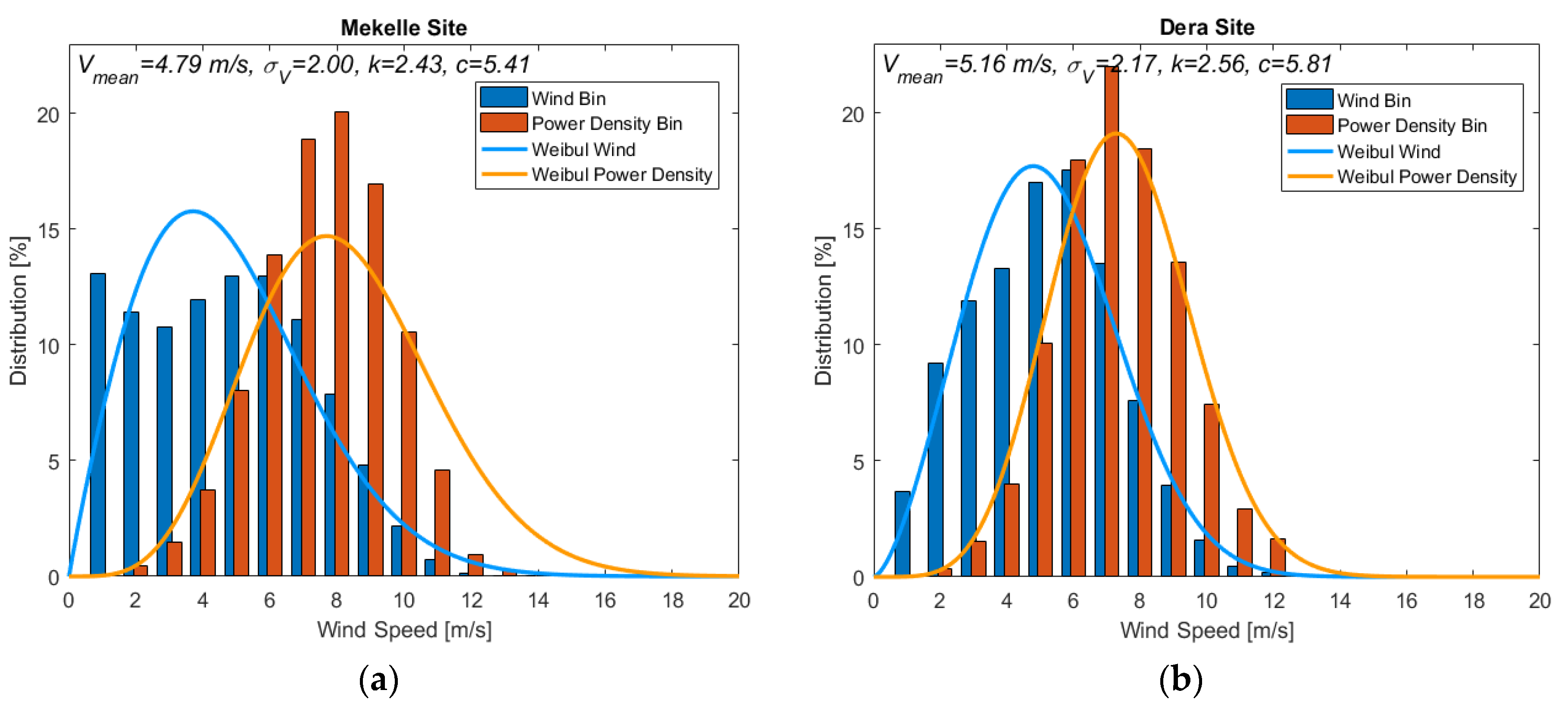
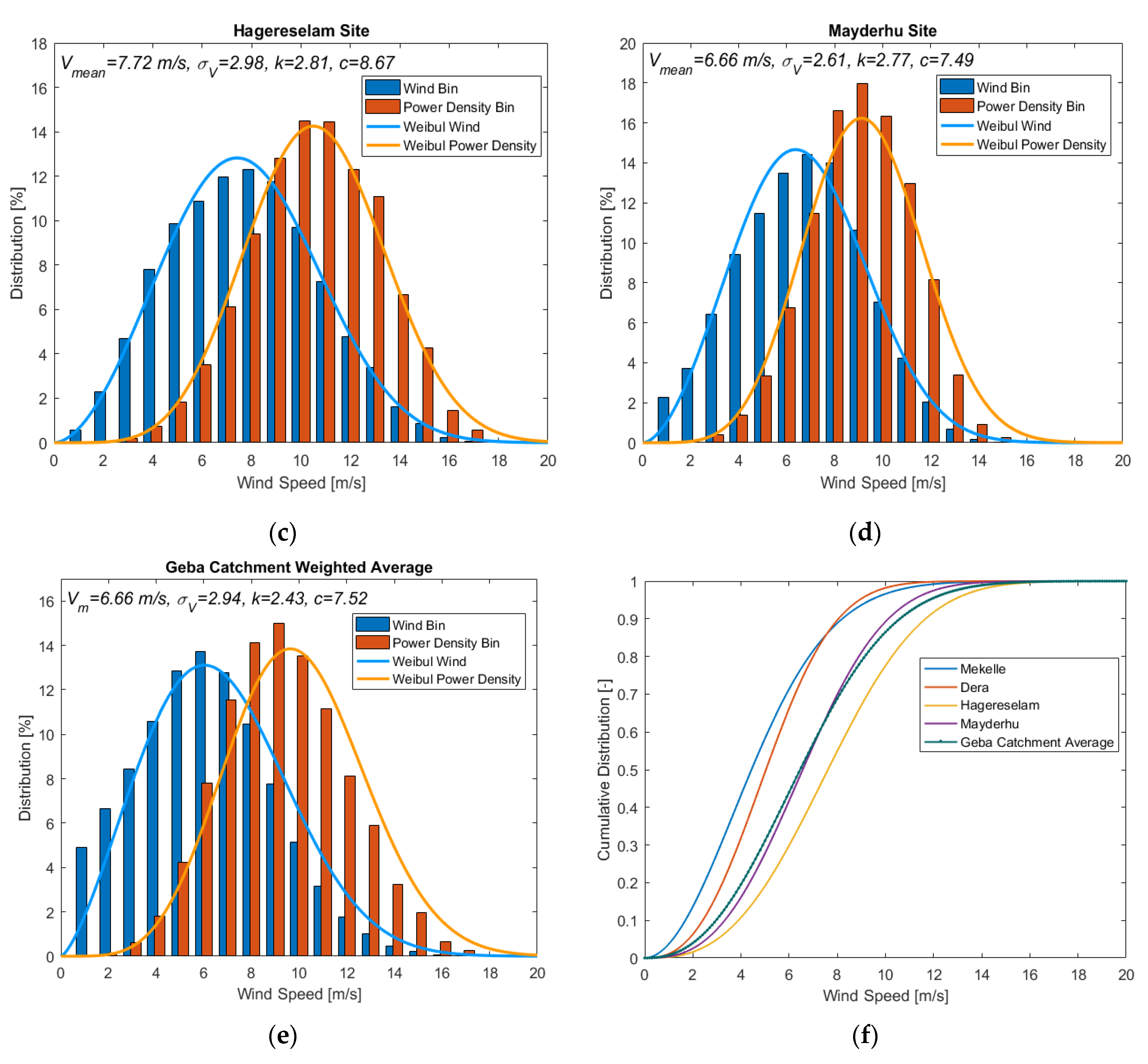
2.2. Wind Resource Characteristics

The bins method will be implemented based on the available records and best practice to summarize wind data. In addition to this, statistical methods are considered as per Manwell [8] to define the wind energy potential of the sites and evaluated the expected turbine productivity of the designed wind turbine. Considering the wind data categorized into N_b bins of width $w_i$, with midpoint wind speeds of $v_i,$ and frequency of occurrence $f_i$, in each bin, the total number of data $N$ is defined as:

$$N={\displaystyle \sum }_i^{N_b}{f}_i$$

(1)

Then the average speed $\overline{V}$ and standard deviation ${\sigma }_V$ of the wind are defined as:

$$\overline{V}=\frac{1}{N}{\displaystyle \sum }_{i=1}^{N_b}{v}_i{f}_i$$

(2)

$${\sigma }_V=\sqrt{\frac{1}{N-1}\left\{{{\displaystyle \sum }}_{i=1}^{N_b}{v}_i^2{f}_i-N{\overline{V}}^2\right\}}$$

(3)

The average power density $\overline{P}/A,$ is expressed as:

$$\overline{P}/A=\frac{1}{2}\rho \frac{1}{N}{\displaystyle \sum }_{i=1}^{N_b}{v}_i^3{f}_i$$

(4)

where $A$ is the swept area of the rotor, and $\rho$ is the density of air.

The average machine power ${\overline{P}}_w,$ and the annual energy production by the rotor are then:

$${\overline{P}}_w=\frac{1}{N}{\displaystyle \sum }_{i=1}^{N_b}{P}_w\left(v_i\right)f_i$$

(5)

$$AEP=E_w={\displaystyle \sum }_{i=1}^{N_b}{P}_w\left(v_i\right)f_i∆t$$

(6)

where $P_w\left(v_i\right)$ is the power produced defined by the power curve of the rotor, and $∆t$ is the time of operation in a year.

In the statistical analysis, the probability distribution is used to describe the likelihood of the occurrence of certain wind speeds. The probability density function defines the probability of occurrence of wind speed between $V_i$ and $V_{i+1}$. There are a few probability distributions in the literature to represent wind behavior. Among these, the Rayleigh and the Weibull are the most often used ones [8]. The Weibull distribution, which needs information of two factors, a shape parameter $k,$ and shape factor $c$, better represents the wind behavior as it incorporates both the exponential and Rayleigh distributions [8,22].

The Weibull probability density function $f\left(V\right)$ and the cumulative distribution function $F\left(V\right)$ are defined as:

$$f\left(V\right)=\left(\frac{k}{c}\right){\left(\frac{V}{c}\right)}^{k-1}exp\left[-{\left(\frac{V}{c}\right)}^k\right], F\left(V\right)=1-exp\left[-{\left(\frac{V}{c}\right)}^k\right]$$

(7)

where the shape parameter $k$, for $1\le k<10$, and the shape factor $c$, are defined as:

$$k={\left(\frac{{\sigma }_V}{\overline{V}}\right)}^{-1.086}, c=\frac{\overline{V}}{\mathsf{\Gamma }\left(1+\raisebox{1ex}{$1$}\!\left/ \!\raisebox{-1ex}{$k$}\right.\right)}$$

(8)

where $\mathsf{\Gamma }\left(1+\raisebox{1ex}{$1$}\!\left/ \!\raisebox{-1ex}{$k$}\right.\right)$ is gamma function defined: $\mathsf{\Gamma }\left(1+\raisebox{1ex}{$1$}\!\left/ \!\raisebox{-1ex}{$k$}\right.\right)={{\displaystyle \int }}_0^{\infty }{e}^{-t}{t}^{\left(1+\raisebox{1ex}{$1$}\!\left/ \!\raisebox{-1ex}{$k$}\right.\right)-1}dt$.

Then, using the statistical methods, an equivalent value of the average machine power Pw in Equation (5), is evaluated as:

$${\overline{P}}_w={\displaystyle \sum }_{i=1}^{N_b}\left\{exp\left[-{\left(\frac{V_{i-1}}{c}\right)}^k\right]-exp\left[-{\left(\frac{V_i}{c}\right)}^k\right]\right\}{P}_w\left(\frac{V_{i-1}+V_i}{2}\right)$$

(9)

which, in turn, is used to calculate capacity factor $CF$ that is a performance parameter of the wind turbine at a specific site, defined as the ratio of the average machine power to the rated power $P_r$ over a given time. Thus:

$$CF=\raisebox{1ex}{${\overline{P}}_w$}\!\left/ \!\raisebox{-1ex}{$P_r$}\right.$$

(10)

2.3. Evaluating Representative Wind Parameters

Design and production of wind turbine blades are expensive for each different nearby sites with different wind resources or wind power production potentials within the same catchment area. Therefore, it is important to design a single blade based on a weighted average parameter of the wind potential of the sites. The weighted average parameter proposed in this paper wasthe wind power density per unit area of the selected sites within the catchment area. Therefore, the proposed weighting factor is:

$$W_j=\raisebox{1ex}{${\left(\overline{P}/A\right)}_j$}\!\left/ \!\raisebox{-1ex}{${{\displaystyle \sum }}_{j=1}^k{\left(\overline{P}/A\right)}_j$}\right.$$

(11)

where $W_j$ is the weighting factor for site $j=1, 2, 3\dots n$, and $n$ is the number of sites within the catchment area with available data.

Then, the representative parameters are the sum of the weighted parameters of each site. For instance, consider the midpoint wind speed of $v_i$, for the bins, the weighted average midpoint wind speeds $v_{ia}$, is:

$$v_{ia}={\displaystyle \sum }_{j=1}^{k_i}{W}_j{v}_i$$

(12)

Based on these, weighted average values of the parameter wind bins, Weibull probability density function, and cumulative distributive function parameters will be available to design and analyze the representative small wind turbine blade.

2.4. Cost of Energy

The cost of energy (CoE) is one of the key parameters required in the design and study of wind turbines, defined as the production cost of unit energy of the rotor [8,20]. Thus:

$$CoE=\raisebox{1ex}{$\left(C_{ce}\times FCR+C_{O\&M}\right)$}\!\left/ \!\raisebox{-1ex}{$AEP$}\right.$$

(13)

where $C_{ce}$ is the capital cost of the wind turbine, $FCR$ is a fixed charge rate, and $C_{O\&M}$ is the operational cost.

In this paper, a variation of lifetime cost is estimated in terms of changes in power rating to evaluate relative-CoE assuming elements of the cost fraction that vary with changes of rated power. Considering this assumption is reasonable for limited scopes related to cost effects. Hence, it is assumed that cost of power electronics varies proportional to the rated power. Blade cost also increases with power rating levels due to more cyclic loads around the rated-power and is likely to vary as to the square root of power [6]. The gearbox is not considered in the scaling analysis as direct-drive small wind turbines are assumed. The costs applied are assuming the component level CoE contribution reported by National Renewable Energy Laboratory (NREL) [23]. Thus, relative-CoE is defined evaluating Equation (13) accordingly as a ratio of nominal CoE value of the respective sites. The rated power corresponding to a relative-CoE of one offers the operation of the blade with minimum CoE at the respective site.

2.5. Selection of Design Parameters

The paper aimed to design a 5 kW small wind turbine with appropriate parameters that suit the selected site conditions. Hence, the use of the best design parameters is very important to maximize the performance of the rotor. Among these, the tip-speed ratio and the number of blades are the most common ones that need careful selection. Hau and Barton et al. illustrates the variances in the efficiencies for rotors of different configurations qualitatively [24,25]. Accordingly, a three-bladed horizontal axis wind turbine at a tip-speed ratio of seven demonstrates maximum efficiency in comparison to the others. Therefore, a three-bladed wind turbine at a tip speed ratio of seven is the selected most efficient combination.

The design wind speed is another parameter that requires careful determination. There are different methods to select the design wind speed. For design considerations based on the wind classes, the International Electro-technical Commission (IEC) standard provides the average wind speeds for each wind class, and the design wind speed recommended is 40% more than the average wind speed [26]. On the other hand, with available wind data for a specific site, the recommended practice is selecting the wind speed at around the highest power density. The practice based on the power density distribution allows us to design the blade at around wind speed corresponding to the highest wind power distribution. It will enable the wind turbine to harness the power at the wind speed with the highest power density at the optimized design. Usually, the mean wind speed of a specific site is slightly higher than the most repeated one. Thus, the design wind speed should be slightly higher than the one that corresponds to the densest wind power. This method of selecting design wind speed is a common practice in the wind-turbine design process [27].

In addition to these density and the kinematic viscosity of air affects the design of wind turbines. For the selected catchment area, these values are taken based on the elevation, annual average temperature, and atmospheric pressure. Therefore, considering the data for environmental conditions of the Geba catchment, an average temperature of 23 °C and an atmospheric pressure of 760 hPa are considered. Accordingly, using the ideal gas law, an average air density of 0.92 kg/m³ and kinematic viscosity of 1.84 × 10⁻⁵ were found.

Airfoils are the major parts of the section requirements of the rotor blade design. These days it is easier to find and use existing airfoils for small wind turbine applications. National Renewable Energy Laboratory NREL (wind.nrel.gov/airfoils) and other similar institutions have been developing some groups of airfoils for wind rotors. The airfoils with decent performance features for small rotors are listed in the literature [15,28,29]. Hence, a set of airfoils of NREL, namely S823 and S822, developed for small wind turbines (2–20 kW) at various conditions, were found appropriate to the sites considered. A rectangular section is selected as the third airfoil to connect the rotor blades with the hub plate at the root part. Lift coefficient C_l, and drag coefficient C_d, at a specific angle of attack α that corresponds to around the maximum lift to drag ratio was taken for the NREL airfoils while the recommended force coefficient by the IEC 61400-2 2006 [26] was considered for the rectangular section.

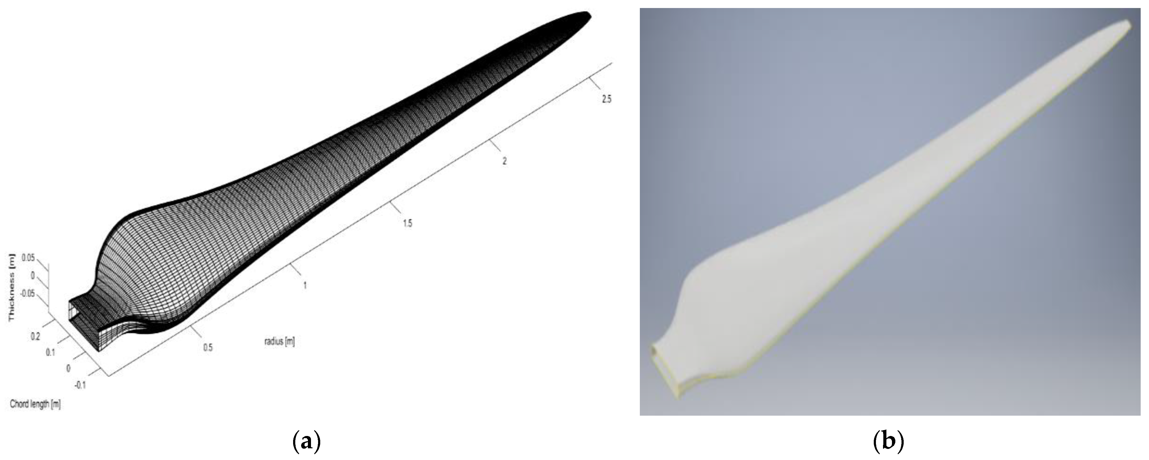
2.6. Blade Element Method and Iterative Process

The BEM is the most typically used method for the aerodynamic and aero-elastic study. Different modifications and improvements have been made, in the design of rotor blades, for better evaluation of forces and velocities. Madson and Dossing explained the BEM [30,31] that is also commonly available in the literature [7,8]. Therefore the modified BEM outlined by Madson and Dossing will be implemented [30,31], in combination with the tip loss factor modified by Shen [32], which is a modification of the Glauert’s tip loss factor that gives an improvement in predicting the aerodynamic forces.

An iterative optimization process has been undertaken in two steps using Matlab code. The first step was the optimization process in the BEM. Here the tangential and axial induction factors have been the constraints required to converge to an ideal value within an acceptable tolerance level. The flow angle or the angle of attack, force coefficients, and element forces were variables to be determined and the tip speed ratio was considered as constant when designing for selected values. Taking the results of the first step as input, the second step considered the design power as the constraint. In the second step, the number of blades, wind velocity, density, and viscosity were the constants while the radius, angular velocity, and chord length were considered as variables.

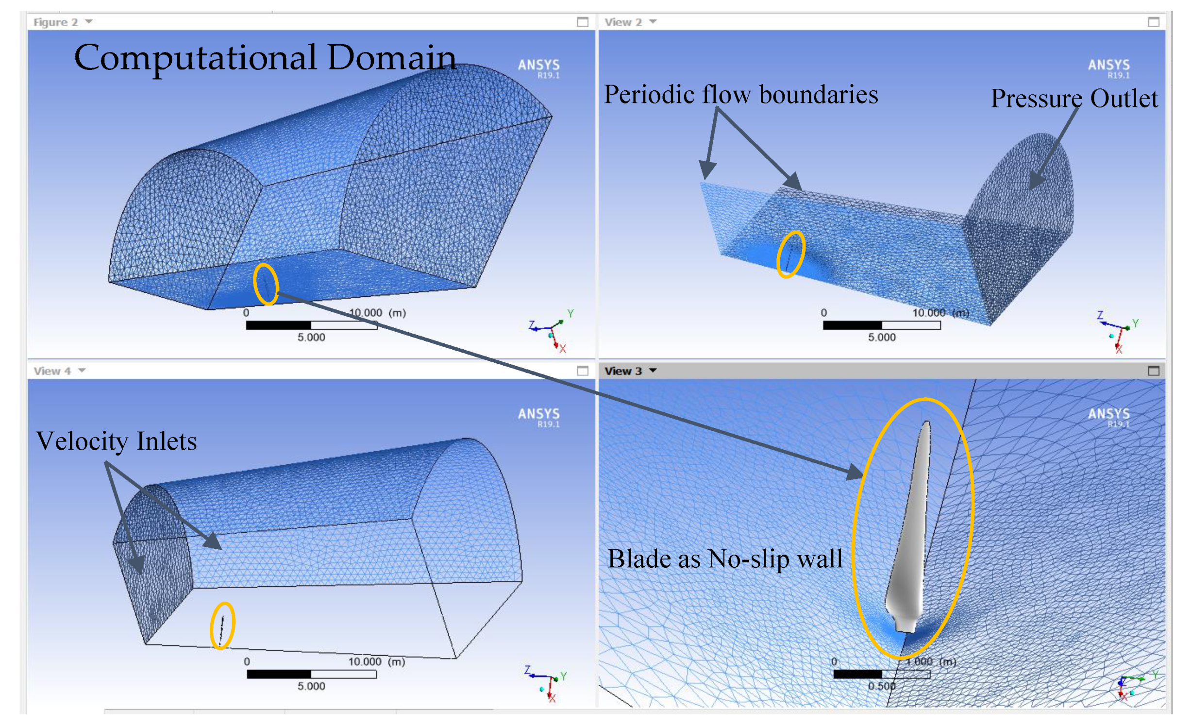
2.7. CFD Modeling and Simulation

Ansys-Fluent, a widely used CFD modeling software, is used for the CFD simulation of the rotor. The CFD modeling considers one-third of a sector of the full cylindrical domain using one blade only with periodic boundary conditions to reduce computation time considerably. Figure 1 shows the boundary conditions and computational-domain of the simulation. The cylindrical computational-domain at the upstream inlet waslocated in front of the blade at three times the blade radius (3R), and its diameter wasfive times the diameter of the blade (5D). On the downstream side, it waslocated at 10R behind the rotor blade with a computational domain cylinder diameter of 7D. These dimensions of the computational domain wereexpected to allow wake expansion and avoid unfavorable boundary dependency effects [33,34]. The rotational frame wasconsidered in the computational-domain to account for the rotor speed, with the blade taken as a non-slip wall boundary condition. Inflation layers of the prismatic type wereused forthe rotor face together with unstructured meshes for the computational-domain to get an improved resolution of the flow in boundary layers to get the wall distance y+ to be less than one [34]. The wall distance y+ is a non-dimensional distance from the wall to the first mesh node used to describe the height of the first grid element next to a wall in a CFD simulation.

In CFD simulations of wind turbine blades, the fluid-flow was analyzed based on the Navier–Stokes equations. RANS equation is investigated usually with either two-equation turbulence models of the k-ε and k-ω series or four-equation shear stress transport k-ω SST turbulence model. The k-ε turbulence model could not depict flows at the boundary layers accurately. It is, therefore, suitable for far-field flow simulations. On the other hand, the k-ω turbulence model could not represent far field flows precisely. Hence, it is appropriate for modeling the boundary layers. The transition k-ω SST turbulence uses the k-ε model and k-ω model alternatively depending on the flow condition. It has the capability of flow separation forecasting on the rotor and reflects the effect of free-stream pressure gradients and turbulence [33,35,36]. Therefore, a four-equation shear stress transport, k-ω SST turbulence model, was employed in the CFD analysis. As per the assessment and investigations of different researchers, the k-ω SST turbulence model was reliable for flow analysis with good agreement with experimental results. However, at large angles of attack, it was confirmed that the CFD simulation results tend to slightly underpredict the power and overpredict the thrust [37,38,39,40,41]. An incompressible analysis was employed, as most of the wind turbine operation is in the subsonic region, with a constant local air density and viscosity. A coupled algorithm for pressure, which considerably increases the convergence rate, was considered in solving the incompressible Reynold-averaged Navier–Stokes (RANS) model [33,42].

Residuals and net mass imbalance were engaged to limit the running time of the solver and ensure convergence. Residuals of the specific dissipation ω, the kinetic energy turbulence k, velocities, and continuity were limited to less than 10⁻⁴ during the solution process. In addition to these, the net imbalance was also checked to be below 0.1% [33,37,43], and an integral static pressure surface monitor to remain constant for a considerable amount of iterations after convergence.

Furthermore, ASHES (simis.io) was employed as an off-design performance evaluation tool. It is a time-domain wind-turbine aerodynamics module, which uses AeroDyne of FAST with a rich user interface. Parameters like a chord, twist angle, pitch axis, airfoil type, and shapefiles of the airfoils at their corresponding radial positions from Matlabwere exported to ASHES as input in the table format. It internally implements xfoil to determine the lift and drag constants for the shapefiles to get the necessary parameters in the evaluation process.

3. Results and Discussion

3.1. Wind Distribution Characteristics and Design Parameters

The wind characteristics of the four sites in the Geba catchment area as bins of power density distribution and wind speed distribution are shown in Figure 2a–d. The figures show also graphs of the Weibull probability wind distribution and power density distribution. Figure 2e shows weighted average distribution over the catchment based on the data from the four sites. Figure 2f shows the corresponding cumulative distribution graphs of the sites the weighted average over the catchment. The results in Figure 2e,f show that the weighted average is close to the wind conditions of the Mayderhu site.

Based on the wind distribution and equations in Section 2.1 and Section 2.2, the parameters for the design of the representative blade were amean wind speed of 6.66 m/s, a standard deviation of 2.94 m/s, a shape factor $k$, of 2.43, and scale factor $c,$ of 7.52 m/s. As can be seen from the plots in Figure 2e, the maximum power density was at a wind speed of around 9.5 m/s, while the most frequent wind was at 6 m/s. Hence, wind speed of 10 m/s was selected as a design wind speed. The range between cut-in wind speed of 2 m/s and cut-out wind speed of 18 m/s was considered as the usable operating range based on the power density distribution. A summary of the design parameters considered is shown in

Table 2. Summary of design parameters.

Design Parameters	Value	Design Parameters	Value
Power (kW)	5	Cut-out wind speed, ${\mathrm{V}}_{\mathrm{co}}$ (m/s)	18
Tip speed ratio, TSR or λ (-)	7	The density of air ρ (kg/m3)	0.92
Number of blades, NBl (-)	3	Kinematic viscosity (m2/s)	1.84 × 10−5
Design wind speed, ${\mathrm{V}}_{\mathrm{d}},$ (m/s)	10	Temperature (°C)	23
Cut-in wind speed, ${\mathrm{V}}_{\mathrm{ci}}$ (m/s)	2	Atmospheric pressure (hPa)	760

.

The output of the blade design analyzed using Matlab code shown in Figure 3a in a 3D plot. Figure 3b shows the same rotor blade after exporting to Inventor as a step file and processed to get the blade surface for further use in the CFD analysis.

3.2. CFD Analysis and Validation

The results of the CFD analysis of the blade sections are shown in Figure 4 at different radial positions from root to the tip. Figure 4 presents velocity streamlines in the left and pressure contours in the right for each section. The flow was fully attached at most of the radial positions except at around the root section. The root part started at r/R = 0.042 and the hub region assumed was up to around 0.115. Along the trailing edge, flow separated at around these radial positions. It was due to the modification of the twist angle out of the optimized values to create a smooth connection to the hub plate. The figure also clearly shows that the angle of attack was close to zero at the tip region and increases towards the root region being maximum at around r/R = 0.115 as a result of the optimum twist angle employed. An almost perpendicular angle of attack was used at the root because of positioning the blade root for proper connection with the hub plate.

Furthermore, the surface pressure contour of the turbine blade shows that pressure distribution was found highest on the pressure side from the tip to around two-thirds of the span along the leading edge. Besides, a lowest pressure was observed on the suction side along the leading edge at similar radial positions. Hence, these differences in surface pressure between the pressure and suction surfaces of the blade created the driving torque with the highest values at around the tip region and decreased while moving towards the root part resulting in smaller pressure differences. It also shows that flow velocity was high on the low-pressure sides and low on the high-pressure sides.

Figure 5 illustrates the limiting streamlines on the pressure and suction sides of the blade at the design conditions. On the pressure side, almost all flows were smooth, and on the suction side, most of the streamlines remained attached to the blade surface except at around the root part. Separation started at the root end and reattached back around r/R = 0.115, which was the point where the optimized twist modification starts creating a connection to the hub plate. Then, the flow will be smooth again along the reattachment line near the trailing edge, as shown in the suction side of the blade. It indicates that the advantage of using twisted small wind turbines to ensure smooth flow.

As a validation process, Figure 6 shows the power coefficient for the variable speed characteristics of the wind turbine applied between the cut-in and cut-out wind speeds of 2–18 m/s, respectively. The corresponding rotational speeds werearound 6.5 rad/s and 32.5 rad/s, respectively. The figure presents the C_P plotof CFD and BEM results at the rated power of 5 kW and rated wind speed of 10 m/s. Accordingly, the CFD results werein good agreement to the BEM results at most of the wind speeds with a slight decrease at high wind speeds. This small deviation of the power coefficient in CFD was due to an increased angle of attack at higher wind speeds, and is an expected kind of variation as discussed in Section 2.7, which was verified by different researchers using experiments. Thus a maximum power coefficient of around 51.8% was achieved at the design/rated wind speed as shown in the figure.

3.3. Performance Evaluation

It is essential to look into different indicator plots to assess the main features of the performance of the designed blade for a range of rotor speeds at different wind speed values. Therefore, Figure 7 and Figure 8 show computed power and torque versus rotor speeds and power coefficient for varying wind speeds.

Figure 7a represents power versus rotational speed for a range of wind speeds. It includes a power curve following the maximum power coefficient C_p-max points until it reached a rated value at the rated wind speed of 10 m/s and the corresponding rotor speed of 307.2 rpm. Beyond the rated wind speed, the power remained at a constant value, which wasthe rated power, moving horizontally to the left, which lowered the rotor speed considering the variable speed operated wind turbine throughout its range. It also shows the maximum power-tracking graph applicable for variable speed generators.

Similarly, Figure 7b shows torque versus rotor speed for the range of wind speeds and operating points of power. Likewise, the operation coincided with the C_P-max locus until it grasped the rated wind speed. All along this curve, rotor speed roseto the rated value. Above the rated wind speed, the operating point moved together with the rated power locus to the stall region. Based on these, it waspossible to generate the power, power coefficient, and rotor speed curves of the turbine to evaluate the performance in terms of AEP and CF of the designed blade.

As a result, Figure 8 shows the variable-speed characteristics of the rotor using the power, power coefficient, and rotor speed against the assumed usable range of wind speeds. In this figure, two different regimes are shown, a maximum-C_p and power regulated regions. The maximum-C_p section spanned from the cut-in wind speed to the rated wind speed of 10 m/s, with maximum turbine C_p at each wind speed. Hence, the C_p was 41.4% at the wind speed of 2 m/s and reached around 51.8% at the rated wind speed. Likewise, the power controlled section ranged from the rated to the cutout wind speed with a constant rated generator power of 5 kW realized by decreasing the rotational speed to a regulated constant value. In this region, the C_p decreased in a parabolic curve to about 8.9% at a wind speed of 18 m/s.

The performance parameters weredetermined by implementing the equations discussed in Section 2.2 (Equations (5), (6), and (10)) to the power curve of the designed blade in Figure 8 and the weighted average wind distribution Figure 2e. The calculated parameters werefound to be the average machine power, ${\overline{P}}_w$ of 1956.1 W, annual energy production, AEP of 17.14 MWh, and power factor, $CF$ of 38.17% considering mechanical efficiency of the blade only, which is C_p. As direct-drive generators wereused in most cases for small wind turbines, assuming a generator efficiency of 97%, for instance, the AEP and $CF$ became 16.63 MWh and 37.03%, respectively.

Consequently, the selected design conditions and processes had led to increased performance of the rotor. Such high performance of small wind rotors, in terms of power coefficient and capacity factor, could be achieved by implementing maximum power tracking control mechanisms together with variable speed generators applying variable speed fixed-pitch operation with assisted stall regulation control strategy.

3.4. Selection of Rated Power for Low Cost of Energy

Now consider the use of the designed blade for the four sites at the designed rated power of 5 kW, and rated wind speed of 10 m/s. The AEP and CF for the sites weredetermined based on the power curve of Figure 8 and the respective wind characteristics of the sites in Figure 2a–d. The results of calculation show AEP of around 8.43, 9.16, 22.55, and 17.01 in MWh with corresponding $CF$ of 18.8%, 20.4%, 50.2%, and 37.9% respectively, for Mekelle, Dera, Hagereselam, and Mayderhu. Then, examining the relationship between AEP, CF, and CoE against rated power for each wind-site, parameters for the optimal use of the blade were assessed. Thus, plots of AEP and CF against rated-power werefound as shown in Figure 9. Generally, the Hagereselam site performed the highest in both parameters; the Mayderhu site delivered moderate performance while Dera and Mekelle delivered low performance.

As a general pattern, the AEP increased with increased rated power while the CF decreased. It is crucial to select appropriate rated-power that can give an advantage to the sites in minimizing the CoE. The optimal power for the respective sites was determined based on the AEP for various rated powers and the relative-CoE considering the suggested cost scaling of the power electronics and blade discussed in Section 2.4. As a result, Figure 10 shows relative-CoE against rated power. Using the turbine at the rated power of 5 kW and rated wind speed of 10 m/s at each site, the relative-CoE increase in comparison to the nominal site value was 3%, 7%, and 1% for Mekelle, Dera, and Hagereselam sites, respectively, and with no change for the Mayderhu site. Therefore, to find the rated power that would give minimum CoE, relative–CoE very close to one was identified for the sites.

Accordingly, using Figure 10, the recommended range of rated power with corresponding rated wind speeds, AEP, and CF of the four sites are shown in

Table 3. Proposed rated power and corresponding parameters of the four sites.

Site	Rated Power (kW)	Rated Wind Speed (m/s)	AEP (MWh)	CF (%)
Mekelle	3–4	8.4–9.3	7.34–7.8	28–22.8
Dera	2.5–3.5	8–8.8	7.94–8.66	36.2–28.2
Mayderhu	3.7–5.3	9–10	15.15–17.2	46.75–37
Hagereselam	5–7	10–11	22.3–25.5	50.9–41.6

. Still the Hagereselam site performed at the top in terms of all the performance parameters, and the Mekelle site wasthe lowest in terms of annual energy production and capacity factor. The Mayderhu site remained at around the design values. On top of the advantage of selecting the rated power that can give low CoE, the use of a single blade design concept had an advantage in minimizing the cost of design and production. If specific blades were considered, for the four sites, four different designs and molds would be leading to at least four times the single blade design and mold cost. Hence, the application of the single blade concept together with selection of appropriate rated power for the respective site minimizes the cost of energy.

In future work, the structural analysis based on the wind conditions considered should be studied, especially for the low wind sites, focusing on determining efficient structure to minimize material and production costs, besides the safety requirements.

4. Conclusions

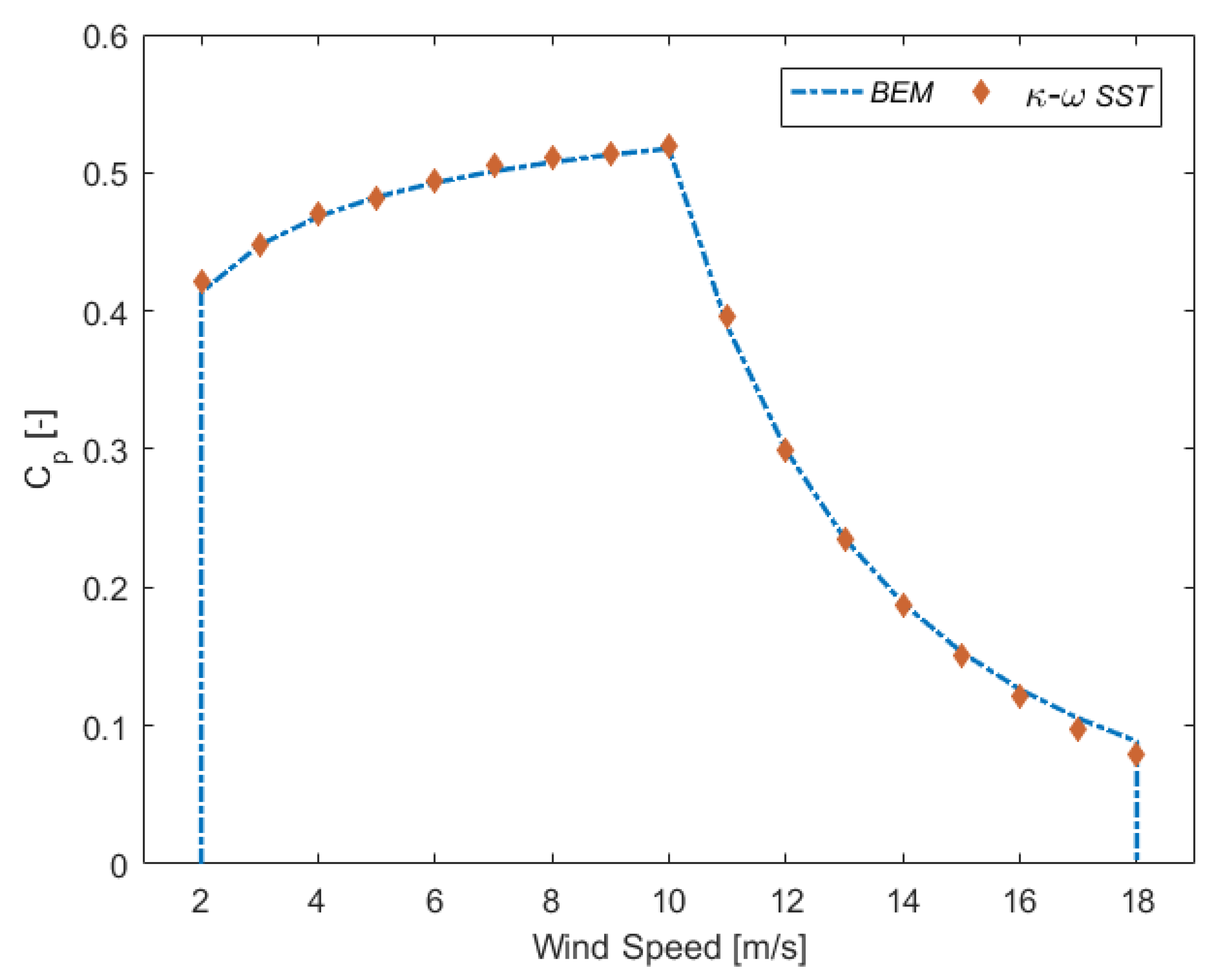
Catchment based aerodynamically optimized small wind turbine was designed using representative wind conditions. The proposed weighting average was based on the wind power density of the wind sites within the catchment area. The blade design was applying the single blade concept and low cost of energy. In designing, BEM was implemented using Matlab code to optimize the local chords, twist angles, radius, and rotational speed of the turbine and exported to Ansys for CFD analysis. Ansys-Fluent was applied to validate the results of BEM, and good agreement found for the power coefficient for a different combination of wind speeds.

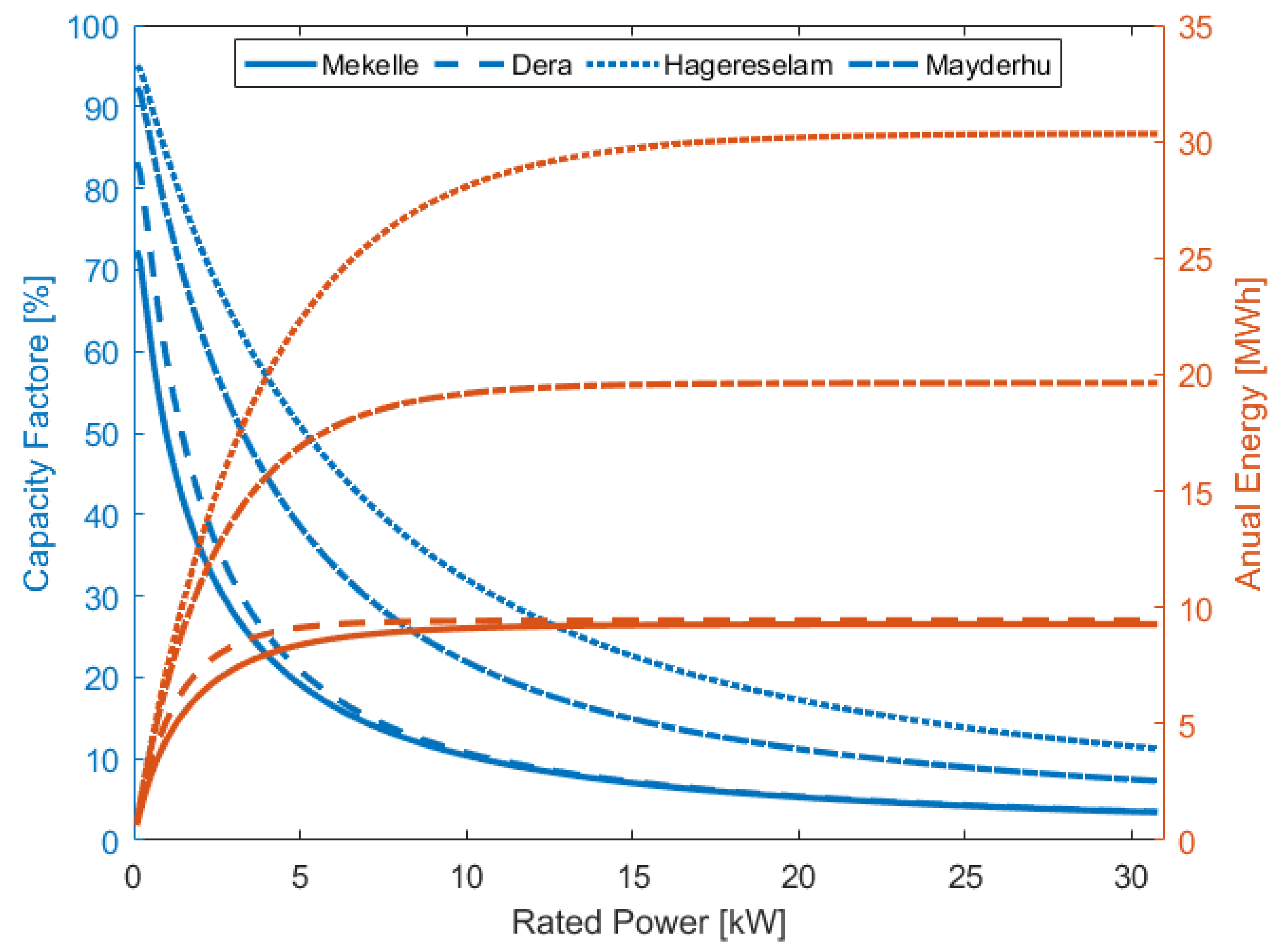
Accordingly, the maximum power coefficient achieved was around 51.8% at a design wind speed of 10 m/s. Considering the single blade concept for all the sites within the catchment area, the performance of the blade at a rated power of 5 kW resulted in capacity factors ranging from 18.8% to 50.2%. Therefore, analyzing the relationship between rated power against annual energy production, capacity factor, and relative cost of energy, a range of appropriate rated power that would give a low cost of energy at higher performances recommended for each site. It can be concluded that for Mekelle and Dera sites, which are low wind sites, rated-powers of 3.5 kW and 3 kW are appropriate at rated wind speeds of 8.8 m/s and 8.4 m/s, performing at capacity factors around 25.1% and 31.8% and corresponding annual energy production around 7.3 and 8.4 in MWh, respectively. While optimum rated-power of 5 kW would be proper for the Mayderhu site at 10 m/s rated wind speed, executing with a capacity factor around 38.6% and annual energy production around 16.9 MWh. On the other hand, as the Hagereselam site is a relatively high wind site, rated power of 6 kW would be proper at 10.5 m/s rated wind speed that would achieve a capacity factor of 45.9% and annual energy production of 24.1 MWh.

Even though the performance of the blade at the Mekelle site was low relative to other wind sites in the catchment, it was moderate to high compared to the most commonly reported wind turbines. On the other hand, the performance at the Hagereselam site was the highest in the catchment area considered and high compared to the existing wind rotors. As the Mayderhu wind condition is very close to the representative weighted average of all sites used for designing the blade, the performance was found very close to the results at design conditions.

In conclusion, it is possible to achieve high performance at a low cost of energy using a single blade concept at appropriate rated power, implementing proper design conditions and procedures for different sites with different wind conditions.

References

1. Barnes, R.H.; Morozov, E.V.; Shankar, K. Improved methodology for design of low wind speed specific wind turbine blades. Compos. Struct. 2015, 119, 677–684. [Google Scholar] [CrossRef]
2. Fuglsang, P.; Bak, C.; Schepers, J.G.; Bulder, B.; Cockerill, T.T.; Claiden, P.; Olesen, A.; Van Rossen, R. Site-specific Design Optimization of Wind Turbines. Wind Energy 2002, 5, 261–279. [Google Scholar] [CrossRef]
3. Soraperra, G. Design of wind turbines for nonstandard air density. Wind Eng. 2005, 29, 115–128. [Google Scholar] [CrossRef]
4. Fuglsang, P.; Thomsen, K. Site Specific Design Optimization of 1.5–2.0 MW Wind Turbines. J. Sol. Energy Eng. 2001, 123, 296–303. [Google Scholar] [CrossRef]
5. Perkin, S.; Garrett, D.; Jensson, P. Optimal Wind turbine Selection Methodology: A Case-Study for Burfell, Iceland. Renew. Energy 2015, 75, 165–172. [Google Scholar] [CrossRef]
6. Jamieson, P.; Hassan, G. Innovation in Wind Turbine Design; John Wiley & Sons Ltd.: Chichester, UK, 2011. [Google Scholar]
7. Hansen, M.O. Aerodynamics of Wind Turbines; Earthscan: London, UK, 2008. [Google Scholar]
8. Manwell, J.F.; McGowan, J.G.; Rogers, A.L. Wind Energy Explained: Theory, Design, and Application; John Wiley & Sons Ltd.: Chichester, UK, 2002. [Google Scholar]
9. Bai, C.J.; Wang, W.C. Review of computational and experimental approaches to analysis of aerodynamic performance in horizontal-axis wind turbines (HAWTs). Renew. Sustain. Energy Rev. 2016, 63, 506–519. [Google Scholar] [CrossRef]
10. Moshfeghi, M.; Song, Y.J.; Xie, Y.H. Effects of near-wall grid spacing on SST-K–ω model using NREL Phase VI horizontal axis wind turbine. J. Wind Eng. Ind. Aerodyn. 2012, 107–108, 94–105. [Google Scholar] [CrossRef]
11. Sørensen, N.N.; Bechmann, A.; Réthoré, P.E.; Zahle, F. Near wake Reynolds-averaged Navier–Stokes predictions of the wake behind the MEXICO rotor in axial and yawed flow conditions. Wind Energy 2014, 17, 75–86. [Google Scholar] [CrossRef] [Green Version]
12. Karthikeyan, N.; Murugavel, K.K.; Kumar, S.A.; Rajakumar, S. Review of aerodynamic developments on small horizontal axis wind turbine blade. Renew. Sustain. Energy Rev. 2015, 42, 801–822. [Google Scholar] [CrossRef]
13. Wind Power as an Alternative to Coal. Available online: https://www.gem.wiki/Wind_power_as_an_alternative_to_coal (accessed on 20 October 2020).
14. Milivojevic, N.; Stamenkovic, I.; Schofield, N. Power and Energy Analysis of Commercial Small Wind Turbine System. In Proceedings of the 2010 IEEE International Conference on Industrial Technology, Vina del Mar, Chile, 14–17 March 2010; pp. 1739–1744. [Google Scholar]
15. Bhatia, S.C. Advanced Renewable Energy Systems Part I; Woodhead Publishing India Pvt Ltd.: New Delhi, India, 2014. [Google Scholar]
16. Danish Wind Industry Association. Available online: http://drømstørre.dk/ (accessed on 25 August 2020).
17. Abdullah, M.A.; Yatim, A.H.M.; Tan, C.W.; Saidur, R. A review of maximum power point tracking algorithms for wind energy systems. Renew. Sustain. Energy Rev. 2012, 16, 3220–3227. [Google Scholar] [CrossRef]
18. Khyam, M.O.; Li, X.; Pesch, D. Sensor Fusion and State estimation of IoT Enabled Wind energy Conversion System. Sensors 2019, 19, 1566. [Google Scholar]
19. Sundev, P.; Anita, J.P.; Sudheesh, P. Nonlinear state Estimation of Wind turbine. In Proceedings of the 2017 International Conference on Advances in Computing, Communications and Informatics (ICACCI), Udupi, India, 13–16 September 2017; pp. 354–358. [Google Scholar]
20. Wang, Z.F.; Tang, X.; Chen, X.S.; Wang, Z.; Wu, J.B. Resource Assessment Report for Wind and Solar Energy of Ethiopia; Chinese Academy of Sciences, Institute of Atmospheric Physics: Beijing, China, 2011. [Google Scholar]
21. Ma, J.T.; Xu, L.S.; Zhao, K. Master Plan Report of Wind and Solar Energy in the Federal Democratic Republic of Ethiopia; Hydrochina Corp: Beijing, China, 2012; Volume 236. [Google Scholar]
22. Lucas, I.A.; Oyama, D.Q.; Alex, M.A.; Augusto, A.C.; Ciro, C.R.; Eduardo, J.A.; Guilherme, J.A.; Weinio, F.A. Analysis of Weibull Parameters for Wind Power Generation. In Proceedings of the 24th ABCM International Congress of Mechanical Engineering, Curitiba, Brazil, 3–8 December 2017. [Google Scholar]
23. Tyler, S.; Beiter, P. 2018 Cost of Wind Energy Review; National Renewable Energy Laboratory: Golden, CO, USA, 2020; NREL/TP-5000-74598. [Google Scholar]
24. Hau, E. Wind Turbines: Fundamentals, Technologies, Application, Economics, 2nd ed.; Springer Science & Business Media: Berlin, Germany, 2006. [Google Scholar]
25. Burton, T.; Jenkins, N.; Sharpe, D.; Bossanyi, E. Wind Energy Hand Book; John Wiley and Sons Ltd. Publication: Chichester, UK, 2011. [Google Scholar]
26. IEC 61400-2. Wind Turbines. Part 2: Design Requirements for Small Wind Turbines; International Electro-Technical Commission: Geneva, Switzerland, 2006. [Google Scholar]
27. Bianchi, F.D.; De Battista, H.; Mantz, R.J. Wind Turbine Control Systems: Principles, Modeling, and Gain Scheduling Design; SpringerVerlag London Limited: London, UK, 2007. [Google Scholar]
28. Timmer, W.A.; Van Rooij, R.P.J.O.M. Summary of the Delft University wind turbine dedicated airfoils. J. Sol. Energy Eng. 2003, 125, 488–496. [Google Scholar] [CrossRef]
29. Giguere, P.; Selig, M.S. Low Reynolds number airfoils for small horizontal axis wind turbines. Wind Eng. 1997, 21, 367–380. [Google Scholar]
30. Madsen, H.A.; Bak, C.; Døssing, M.; Mikkelsen, R.; Øye, S. Validation and modification of the Blade Element Momentum theory based on comparisons with actuator disc simulations. Wind Energy 2010, 13, 373–389. [Google Scholar] [CrossRef]
31. Døssing, M.; Madsen, H.A.; Bak, C. Aerodynamic optimization of wind turbine rotors using a blade element momentum method with corrections for wake rotation and expansion. Wind Energy 2012, 15, 563–574. [Google Scholar] [CrossRef]
32. Shen, W.Z.; Mikkelsen, R.; Sørensen, J.N.; Bak, C. Tip Loss Corrections for Wind Turbine Computations. Wind Energy 2005, 8, 457–475. [Google Scholar] [CrossRef]
33. Wang, L.; Quant, R.; Kolios, A. Fluid0-structure interaction modeling of horizontal-axis wind turbine blades based on CFD and FEA. J. Wind Eng. Ind. Aerodyn. 2016, 158, 11–25. [Google Scholar] [CrossRef] [Green Version]
34. Hansen, M.O.L.; Sørensen, J.N.; Voutsinas, S.; Sørensen, N.; Madsen, H.A. State of the art in wind turbine aerodynamics and aeroelasticity. Prog. Aerosp. Sci. 2006, 42, 285–330. [Google Scholar] [CrossRef]
35. Sørensen, N.N.; Michelsen, J.; Schreck, S. Navier–Stokes predictions of the NREL phase VI rotor in the NASA Ames 80ftx120ft wind tunnel. Wind Energy 2002, 5, 151–169. [Google Scholar] [CrossRef]
36. Mo, J.-O.; Lee, Y.-H. CFD Investigation on the aerodynamic characteristics of a small-sized wind turbine of NREL PHASE VI operating with a stall-regulated method. J. Mech. Sci. Technol. 2012, 26, 81–92. [Google Scholar] [CrossRef]
37. Choi, N.J.; Nam, S.H.; Jeong, J.H.; Kim, K.C. Numerical study on the horizontal Axis turbines arrangement in a wind farm: Effect of separation distance on the turbine aerodynamic power output. J. Wind Eng. Ind. Aerodyn. 2013, 117, 11–17. [Google Scholar] [CrossRef]
38. Lanzafame, R.; Mauro, S.; Messina, M. Wind turbine CFD modeling using a correlation-based transitional model. Renew. Energy 2013, 52, 31–39. [Google Scholar] [CrossRef]
39. Tachos, N.S.; Filios, A.E.; Margaris, D.P.; Kaldellis, J.K. A computational aerodynamics simulation of the NREL phase II rotor. Open Mech. Eng. J. 2009, 3, 9–16. [Google Scholar] [CrossRef]
40. Hsiao, F.B.; Bai, C.J.; Chong, W.T. The performance test of three different horizontal axis wind turbine (HAWT) blade shapes using experimental and numerical methods. Energies 2013, 6, 2784–2803. [Google Scholar] [CrossRef] [Green Version]
41. Li, Y.; Paik, K.J.; Xing, T.; Carrica, P.M. Dynamic overset CFD simulations of wind turbine aerodynamics. Renew. Energy 2012, 37, 285–298. [Google Scholar] [CrossRef]
42. ANSYS, Inc. 2019 R2. Canonsburg, PA, USA. Available online: http://www.ansys.com (accessed on 25 August 2020).
43. Bourdin, P.; Wilson, J.D. Windbreak aerodynamics: Is computational fluid dynamics reliable? Bound. Layer Meteorol. 2008, 126, 181–208. [Google Scholar] [CrossRef]
Figure 1. Computational-domain and boundaries of the computational fluid dynamics simulation.
Energies 13 05838 g001
Figure 2. (ae) Wind distribution and wind power density and (f) cumulative distribution of the selected.
Energies 13 05838 g002aEnergies 13 05838 g002b
Figure 3. 3D geometry of the designed blade: (a) using Matlab and (b) using Inventor.
Energies 13 05838 g003
Figure 4. Velocity streamlines and pressure contour of the blade sections at a different radial positions from the root to the tip.
Energies 13 05838 g004aEnergies 13 05838 g004bEnergies 13 05838 g004c
Figure 5. Limiting streamlines of the blade surface at the design condition.
Energies 13 05838 g005
Figure 6. Power coefficient vs. wind speed of the designed blade for an operating range of the selected sites.
Energies 13 05838 g006
Figure 7. (a) Power vs. rotor speed including maximum power graphs for variable speed operation of the designed blade and (b) torque vs. rotor speed, including maximum power graphs for variable speed operation of the designed blade.
Energies 13 05838 g007aEnergies 13 05838 g007b
Figure 8. Power coefficient, power, and rotational speed, vs. wind speed of the designed blade for the operating range.
Energies 13 05838 g008
Figure 9. Annual energy production and capacity factor vs. rated power of the designed blade at the selected sites.
Energies 13 05838 g009
Figure 10. A relative cost of energy vs. rated power of the designed blade at a ratio of nominal rating of the respective sites.
Energies 13 05838 g010