3.1. Effect of Temperature on the Phase Angle Values
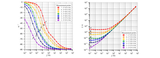
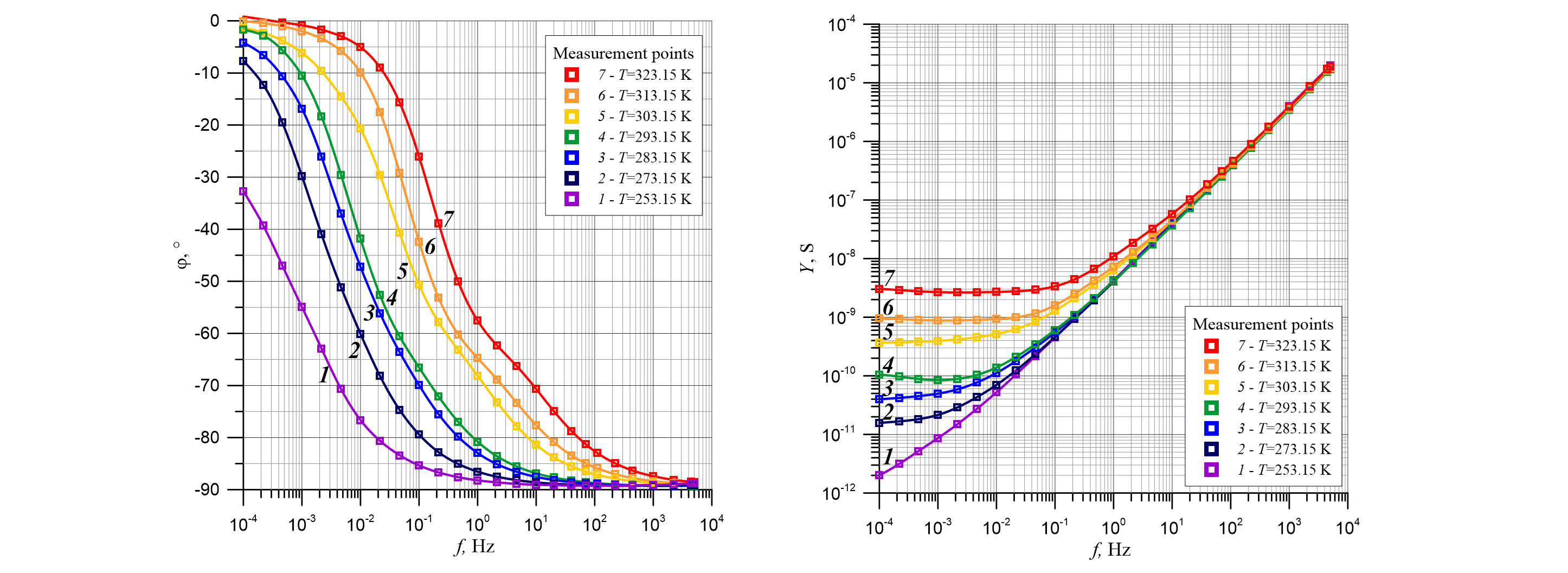
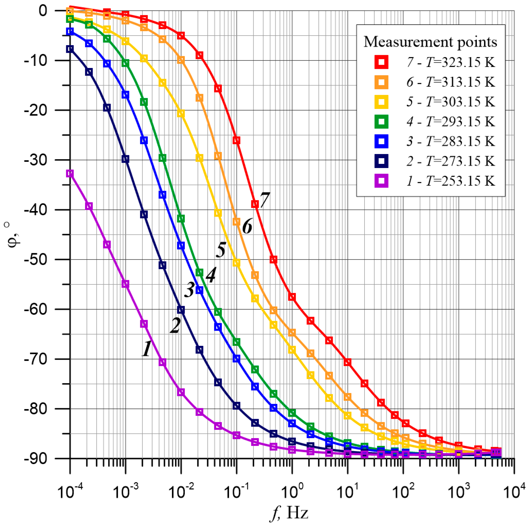
Figure 2 shows the frequency dependence of the phase shift angle of the cellulose composite, synthetic ester, and water nanoparticles measured at measurement temperatures of 253.15 K, 273.15 K, 283.15 K, 293.15 K, 303.15 K, 314.15 K, and 323.15 K.
As can be seen from the picture, measuring points were relatively rarely located, i.e., three per decade. This was because the need to perform time-consuming measurements in the ultra-low frequency area. Indeed, at a measuring frequency of 0.0001 Hz, a single alternating voltage change interval was 10,000 s, i.e., about 2.77 h. In order to perform an accurate analysis of the waveforms shown in
Figure 2, the values of the phase shift angles between measuring points were necessary. In order to obtain intermediate values between measuring points, polynomial approximation of experimental courses was performed (
Figure 2). The approximation was performed using method proposed in a previous study [
27]. The use of polynomial approximation is often associated with the appearance of oscillations between the approximation nodes at the end of an approximation range. To avoid their manifestation, the measurement data was extrapolated using a linear function below and above the range of measurement points. The use of measurement data extrapolation made it possible to shift approximation oscillations into a range of added extrapolation points. Thanks to this procedure, oscillations did not occur in the range of measurement data, thus enabling precise data analysis.
The results of the approximation are presented in
Figure 2 in the form of continuous lines. Each of these lines consists of 200 points per decade, which was obtained by approximation. The following two arguments prove the high quality of approximation. First, values of determination coefficients R
2 were presented in
Table 1. As
Table 1 shows, the values of determination coefficients R
2 for runs, obtained for all measurement temperatures, were close to unity. The lowest value, obtained for the measurement temperature
T = 303 K, was R
2 = 0.999996, proving a very high quality of polynomial approximation performed with a method proposed in a previous paper [
27].
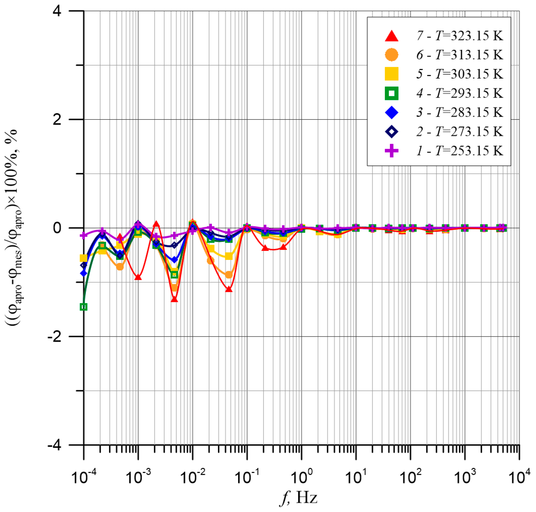
The second argument is the differences between experimental values and approximation results, expressed in percent and shown in
Figure 3. The figure shows that the biggest differences are observed in the range of lowest frequencies and highest temperatures, as well as that their values do not exceed 1.5%. This is a highly satisfactory result.
Figure 2 shows that the phase shift angle for the lowest measurement frequency 10
−4 Hz was close to zero. This means that conductivity at low frequencies for these temperatures (i.e. 283.15 K, 293.15 K, 303.15 K, 314.15 K and 323.15 K) is mostly resistive. Only when the measurement temperature was 253.15 K did the phase shift angle at 10
−4 Hz become greater than -32°. In this case, there was also the capacitive component of the complex conductivity.
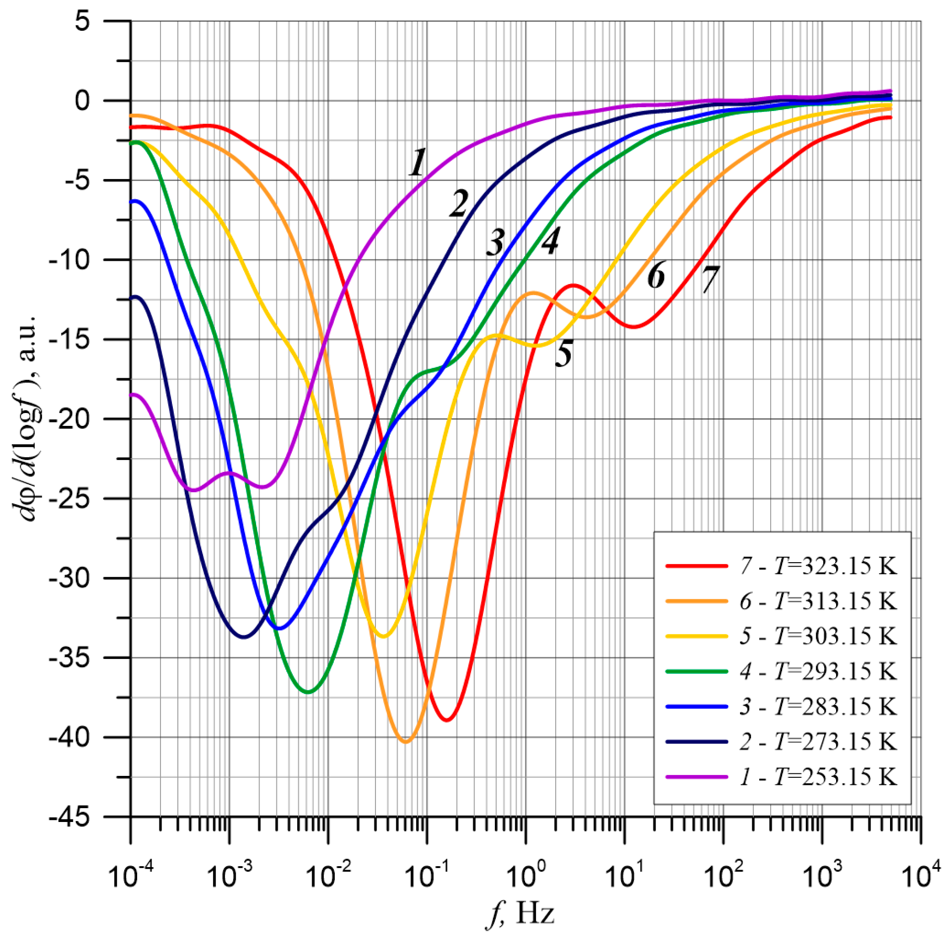
As the frequency increases, especially at temperatures of 283.15 K and above, the module value of the phase shift angle increased more rapidly. At a certain frequency, the value depends on the measuring temperature. This process can undergo certain refraction; for example, for measuring a temperature of 323.15 K at a frequency of about 0.3 Hz. At this point, the curve clearly changed its slope and slowly began moving to a value of −90°, which is characteristic of this type of capacitive conductivity. In order to show such a trend, the values of
dφ(f)/d(log
f) were calculated on the basis of approximations of
dφ(
f)/
d(log
f) derivatives, which are shown in
Figure 4.
We analyze the waveforms of the derivative
dφ(
f)/d(log
f), shown in
Figure 4, using the example of a waveform at a measurement temperature of 323.15 K. The first derivation of the function allowed us to determine the places of fastest change for the function. For the decreasing function, which was the dependence of the phase shift angle on the frequency, it was the minimum position. At this point, the rate of change of the angle of the phase shift was obtained by the maximum value. For the point with the slowest function change, there was a maximum value of the derivative.
Figure 4 shows that the frequency dependence of the phase angle of shift was based on two distinct minima at frequencies of about 0.1 Hz and 10 Hz. They were separated from each other by a clear maximum, which was about 2 Hz. Changes in the phase angle with frequency took place in two stages. The low-frequency stage was characterized by a faster phase shift angle change than the high-frequency stage 2. This was due to the fact that the depth of the first minimum was more than twice as fast than the second minimum. The waveforms obtained for the remaining measurement temperatures showed two minima and one maximum separating them, the positions of which moved into the area of lower frequencies with a temperature decrease. The lower the temperature, the less the minimum was visible at a higher frequency. As shown in the
Figure 2, at 253.15 K the downward path differs significantly from the other temperatures. On this waveform (
Figure 4, curve 1), in the low frequency region, there are two closely spaced minima of almost equal values with much smaller depths compared to the minima for temperatures of 273.15 K and above. In our opinion, at this temperature the water was solid, which changed the electrical parameters of ice compared to liquid water. During the transition from liquid to solid, the dielectric permittivity and conductivity of water decreased. This undoubtedly impacted the phase shift angle, which can be seen in the phase shift angle (
Figure 2) and its derivative of the frequency logarithm (
Figure 4). After water transitioned to liquid at 253.15 K, the phase shift angle curves and its derivative significantly differed from water in a liquid state. We did not consider the curves obtained at 253.15 K.
Slope change in the frequency range of 0.3 Hz is clearly visible in
Figure 5, where the dependence of the phase shift angle module, measured at the temperature 323.15 K, on the frequency in double logarithmic coordinates is shown. For the frequencies below 0.3 Hz, the smallest squares of the course is given by the following formula:
The factor R² = 0.9855 indicates high quality approximation. The second part, above 0.3 Hz, is described by the formula:
The R² coefficient in this case is 0.9638. Similar results were obtained for the remaining measurement temperatures.
The refraction and slowing down of φ(
f) in the higher frequency areas, as shown in
Figure 2,
Figure 4, and
Figure 5, indicate that there are two mechanisms of dielectric relaxation in cellulose composites: synthetic ester and water nanoparticles. The first is characteristic for low and ultra-low frequency areas. The second is found in higher frequency areas.
An increase in temperature causes a shift in high frequency areas (
Figure 2). This is related to a decrease in activation energy for the relaxation time of the phase shift angle [
31,
32]:
where Δ
Wφ is the activation energy for the relaxation time of the phase shift angle and
τ0 is the numerical factor.
The FDS meter does not directly measure relaxation times. On the basis of FDS testing, the value of the relaxation time can be determined with the numerical factor
τ0 by analyzing the phase shift angle after temperatures rise into higher frequency areas (
Figure 2). For this purpose, we selected a specific value of the phase shift angle and read the frequencies, at which this value occurred at different temperatures. The relaxation time value, to the nearest unspecified constant value, was identical for all temperatures (see Formula (4)) and determined by the following formula:
where
τ(T) is actual relaxation time,
φi is the selected value of the phase shift angle,
τ0 is a more or less undefined constant value equal for all temperatures, and
f(T,
φi) is the frequency at which the selected value of the phase shift angle occurs.
In order to precisely determine the activation energy for the relaxation time of the phase shift angle
φ(f), 15 values of the phase shift angle from −10° to −80° with a step of 5° were selected. Selecting such a large number of displacement angles allows for the determination of activation energy in a wide frequency range, as well as for high accuracy calculation of mean value and measurement uncertainty.
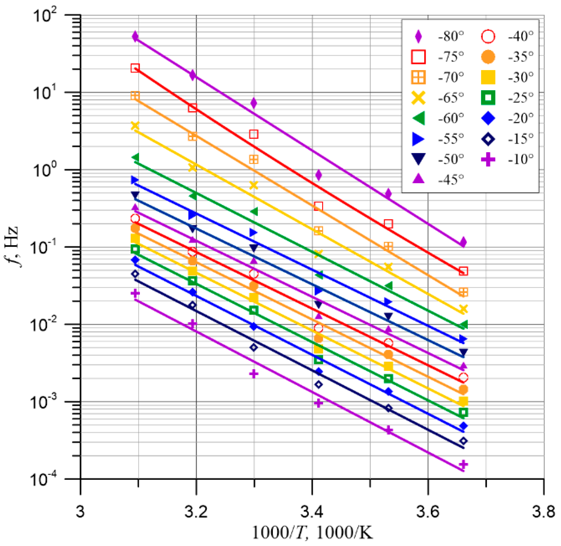
Figure 6 shows Arrhenius’ diagrams for the frequency
f(T, φi) with 15 selected values of
φi as a function of inverse 1000/
T temperature and the results of their linear approximation using the least squares method. The approximation waveforms are almost parallel for different values of phase shift angles. This means that the corresponding values of activation energy for relaxation times are close to each other. The determination coefficients R
2 obtained for the approximation waveforms are shown in
Table 2. As can be seen, the values of R
2 range from 0.9499 to 0.9794. These results are close to unity, which indicates a high quality of linear approximation. On the basis of approximation formulae, activation energy values for relaxation times were determined for all values of phase shift angles from −10° to −80°. The activation energy values for relaxation times in the phase shift angle are shown in
Table 2 and
Figure 7. The mean values of activation energy, determination factors R
2, and standard deviation were calculated from 15 residual values, as presented in
Table 2.
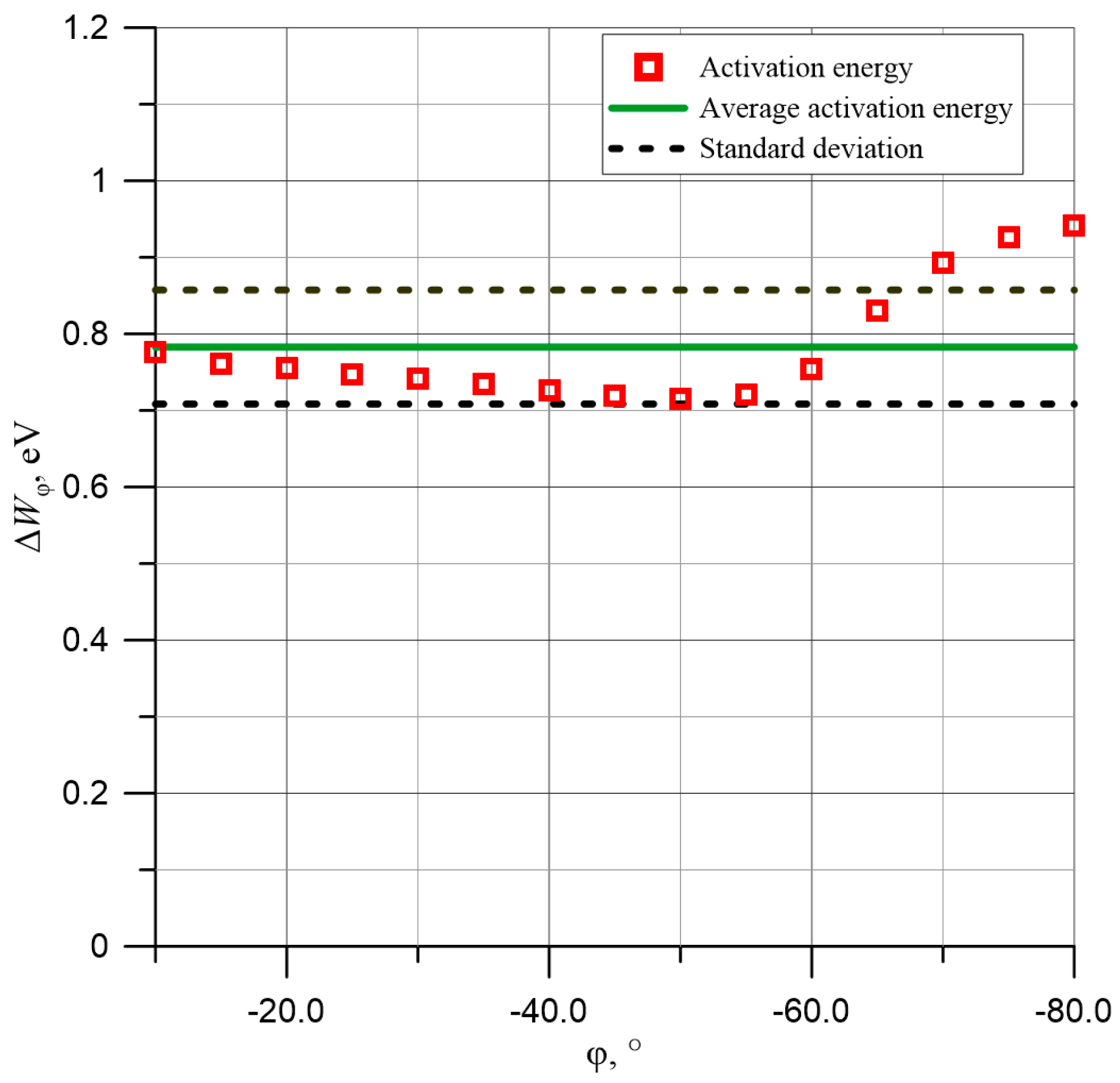
As can be seen from
Table 2, the average value of the activation energy for the relaxation time of the phase shift angle is Δ
Wφ ≈ (0.783 ± 0.0744) eV.
Figure 7 shows that only in the area of the highest values of the phase angle module the activation energy slightly exceeds the mean value plus standard deviation. This may be due to the fact that starting from the value phase shift angle of −70°, the slope of the φ(
f) curves decreases (
Figure 2). This lowers the accuracy of determining the frequency values at which the phase shift angles selected for the activation energy calculation can occur. These inaccuracies can be seen in
Figure 6 for large values of φ.
3.2. Effect of Temperature on the Admittance Value
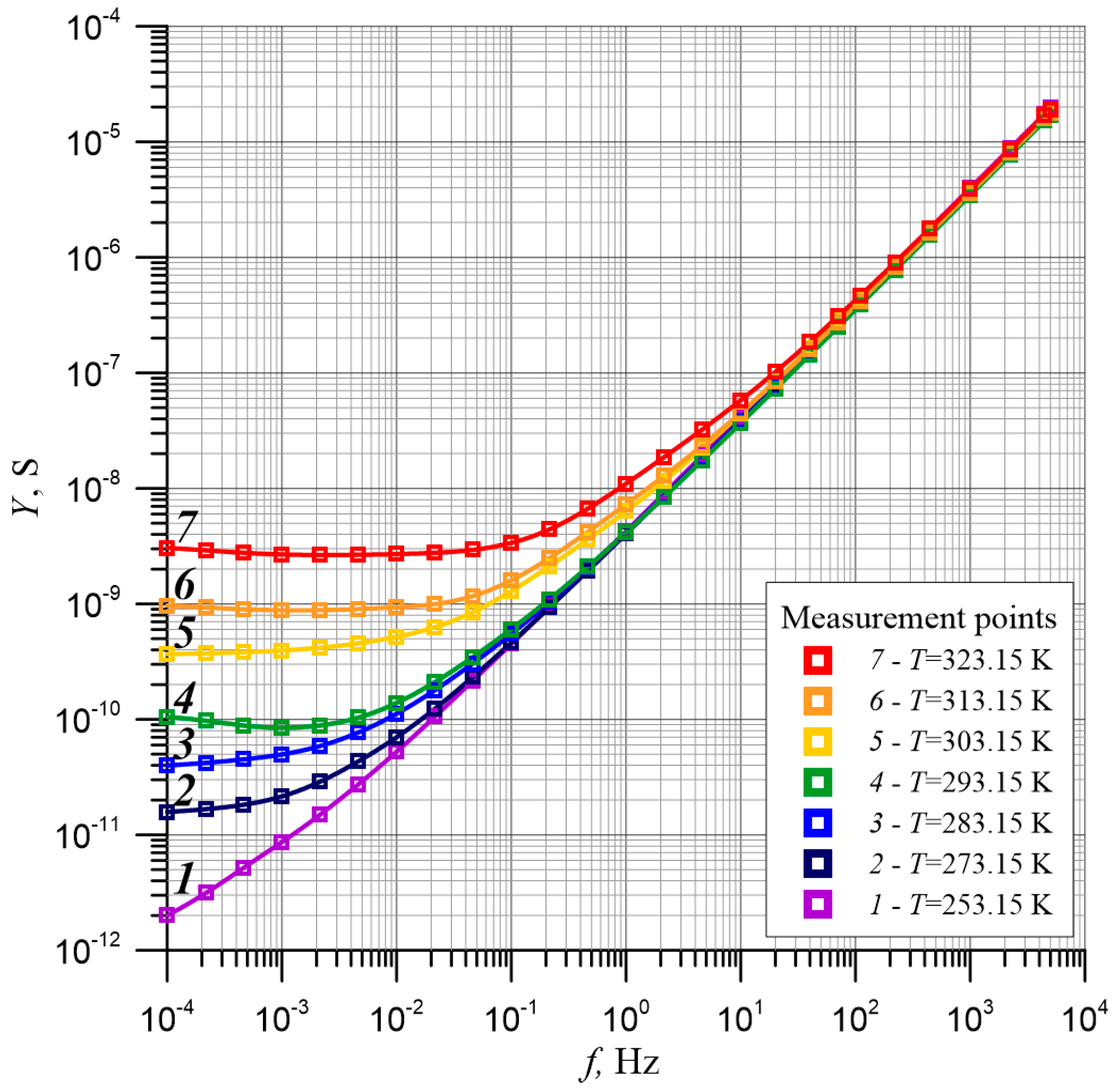
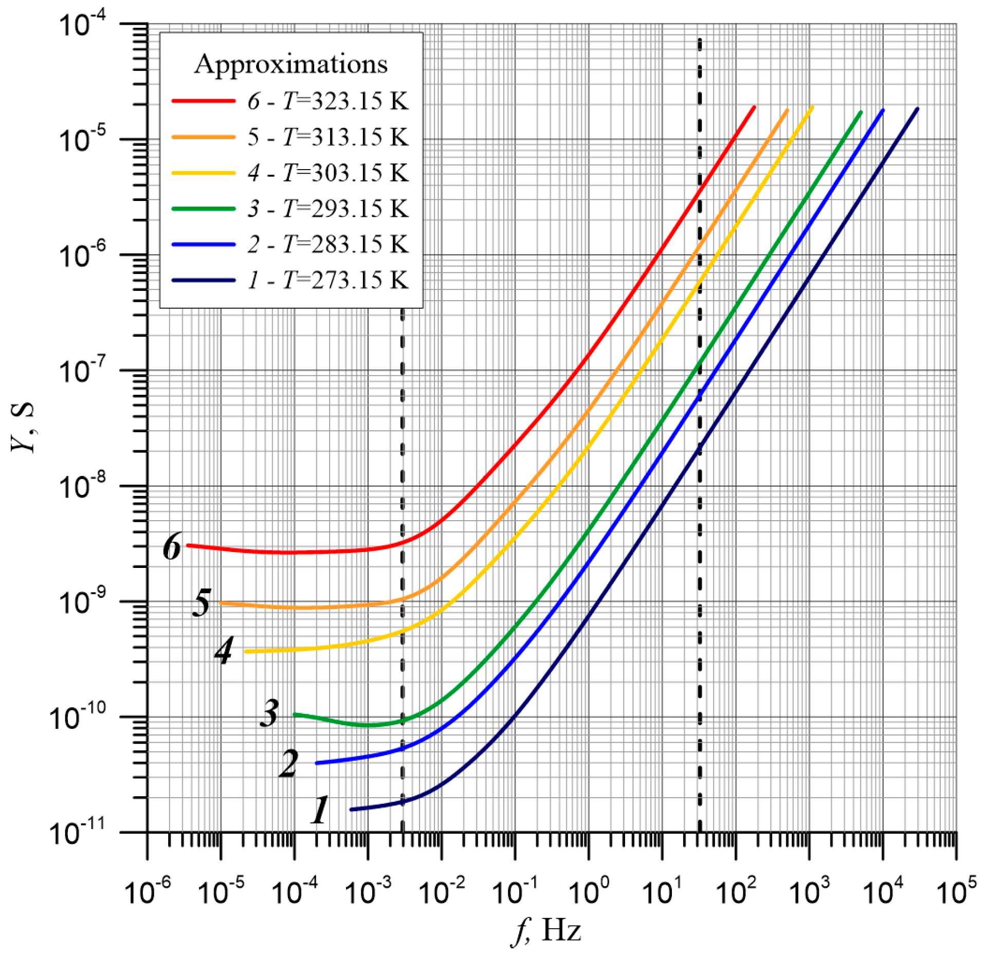
Figure 8 shows, in the form of cellulose composite admittance values, synthetic ester and water nanoparticles measured at temperatures between 253.15 K to 323.15 K. As can be seen from
Figure 8, in the ultra-low frequency area for each temperature, except 253.15 K, the admittance value did not depend on the frequency. In this frequency area, the admittance value only depended on the temperature and not relaxation time. As the frequency increased further, the admittance value increased. As the temperature increased, it moved to a higher frequency area. This was due to the change in relaxation time as temperature increased. The analysis of the experimental results shown in
Figure 8 show that the conductance value in the ultra-low frequency area depend on temperature. In the high frequency area, there was an influence of temperature on the relaxation time changes. However, the curve for 253.15 K behaved differently than the others. This may be due to the fact that 253.15 K was 20 K lower than the freezing point. Therefore, in a further analysis of the results, this curve was not considered.
Similar to the phase shift angle value, the experimental results were approximated using the polynomial method and are presented in
Figure 8 with continuous lines [
27]. The values of determination factor R
2 for the processes approximated by admittance are presented in
Table 1. As can be seen, these values are close to unity. This proves a high approximation quality.
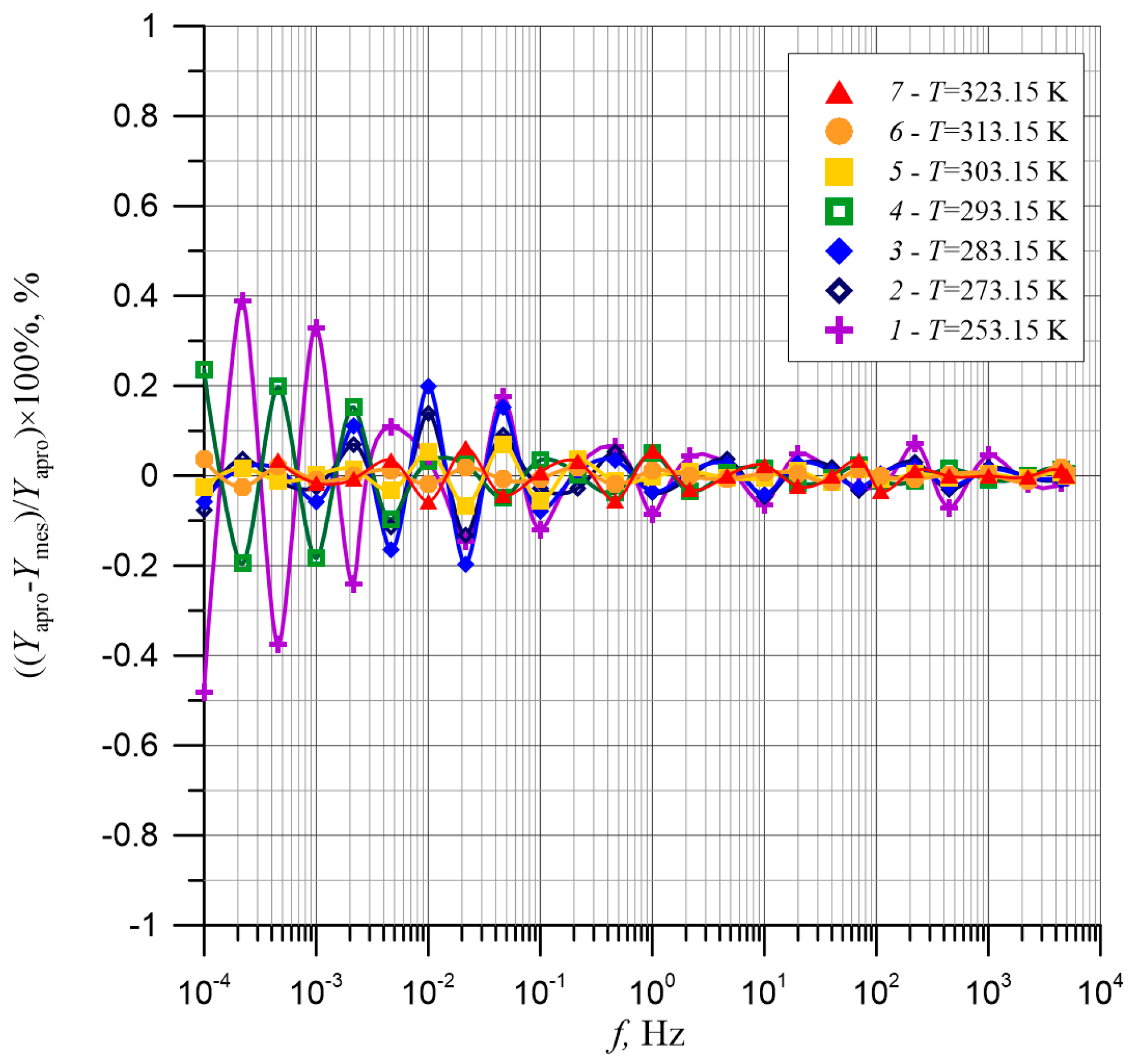
Figure 9 shows the percentage differences between the approximation and experimental results. As shown in
Figure 9, these differences in the ultra-low frequency area did not exceed 0.45% and decreased with increasing frequency. This indicates a very high quality of polynomial approximation.
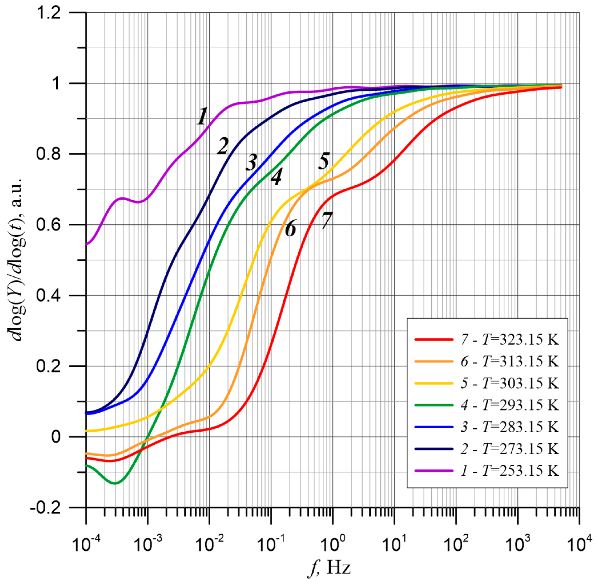
Figure 10 shows the values of
d(log
Y)/
d(log
f) derivatives, obtained after differentiating the approximation, as shown in
Figure 8.
The curve for the temperature 253.15 K differed significantly from others. There was a clear minimum around 8 × 10⁻⁴ Hz. On the remaining runs, only slowdowns were visible. Therefore, similarly to the analysis of the phase shift angle, the curve for the temperature 253.15 K was not considered when calculating the activation energy.
The position of the admittance waveforms in the double logarithmic coordinates was simultaneously influenced by the temperature dependence of the admittance value and admittance relaxation time. In the ultra-low frequency region, DC conductivity occurred. This was evidenced by
Figure 2, from which it can be seen that for temperatures of 273 K and above, the phase shift angle was close to zero degrees. It follows that in this frequency region the admittance was determined by the resistance and its values did not depend on relaxation time. Its value depended only on the temperature through DC conductivity activation energy, given by the formula [
33,
34]:
where
σ(T) is DC conductivity,
σ0 is constant value, Δ
W is DC conductivity activation energy,
k is Boltzmann constant, and
T is temperature
The influence of the temperature dependence on the admittance value is clearly visible in the lowest frequency area of
Figure 8. In this frequency range, for temperatures of 273.15 K and higher, the values of admittance did not depend on the frequency. This means that, in this frequency area, the admittance value did not depend on relaxation time. On the other hand, the increase of the admittance value with the increase in temperature was a result of the activation energy’s influence on admittance. In the ultra-low frequency area, including the frequency of 10
−4 Hz, the admittance value depends on the temperature through the activation energy of admittance value. This eliminates the influence of the activation energy on admittance over the course of the admittance. Therefore, the Y(
f) runs at 273.15–323.15 K were shifted to 293.15 K. The reference temperature in electrical engineering were 10
−4 Hz and had equal admittance values (
Figure 11). After such a shift, only the temperature dependence of the relaxation time had an effect on the waveforms shown in
Figure 11.
For admittance analysis, the quantum phenomenon of electron tunneling between water droplets was used in this study. In [
23], a relaxation time formula for electron tunneling was derived:
where
β is numerical coefficient (the value of which, according to [
35] was
β ≈ (1.75 ± 0.05)),
r is the distance between the wells of potentials produced by the nanodrops of water,
RB is the Bohr radius for the hopping electron, ∆
WY is the activation energy of admittance, and
r0 is the numerical coefficient.
The measurement results, shown in
Figure 11, were made for a sample containing 5% of moisture. This means that the average distance between the water nanoparticles was a constant value. Taking this fact into account, Formula (6) can be converted into:
where:
Formulas (7) and (8) show that in the tested sample, due to the constant concentration of potential wells—i.e., nanodrops of water—the relaxation time reduced to the known Formula (3) and depended only on temperature.
On the basis of FDS admittance measurements, we determined the relaxation time value with the accuracy of the numerical factor
τ0. For this purpose, the temperature shift of the admittance flows into a higher frequency area were analyzed. To determine the relaxation time value, we selected a specific value of admittance
Yi (
Figure 11) and then read the frequency values at which this value occurred at different temperatures. The value of the relaxation time, to the nearest unspecified constant value, were identical for all temperatures (see Formulas (7) and (8)), which were determined by the formula:
where
f(Yi) is the frequency at which the value of admittance
Yi at different temperatures occurs,
τ(
T) is the actual relaxation time, and τ
0 is an unspecified constant value equal for all temperatures.
In
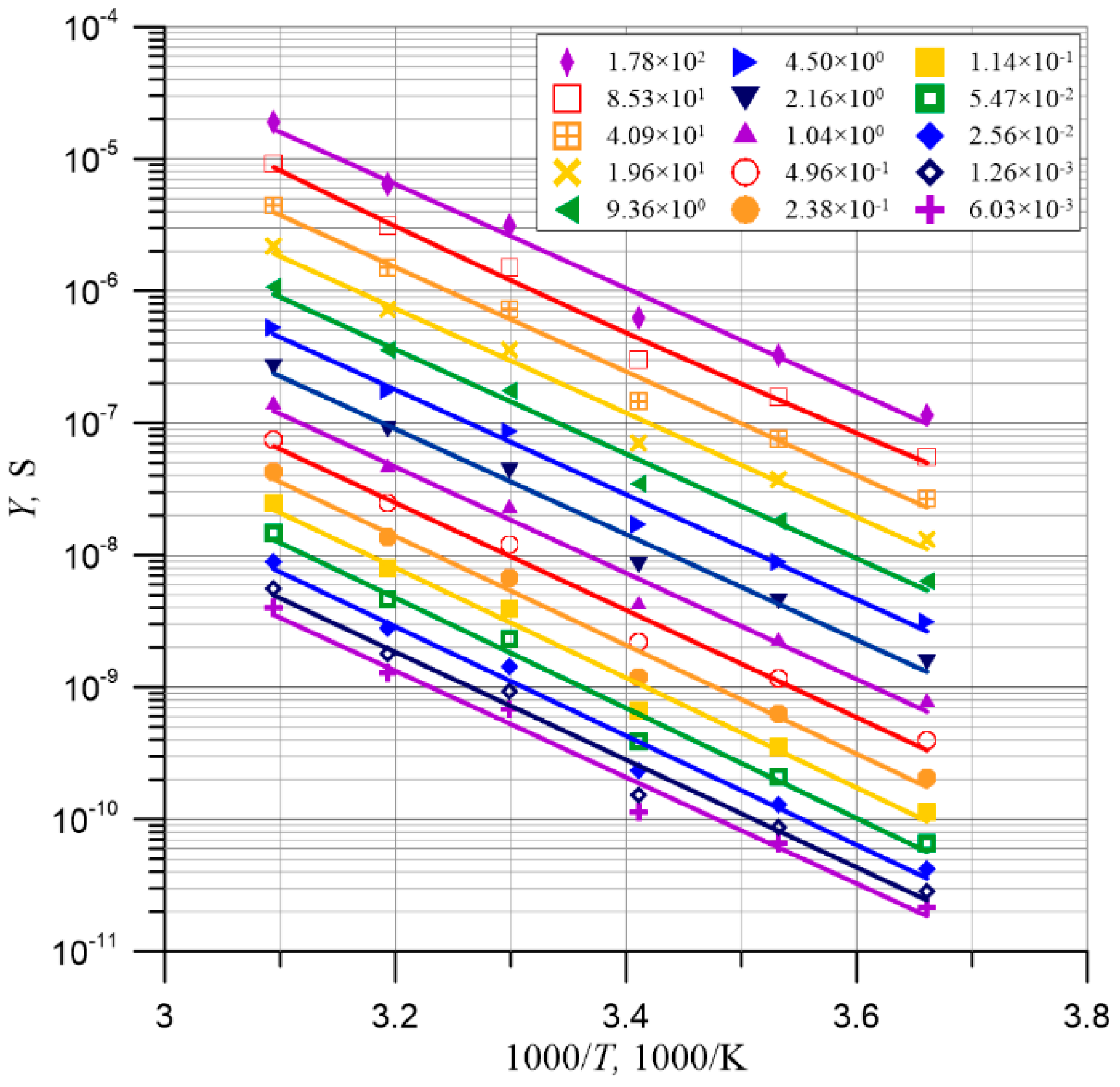
Figure 11, the area of changes in conductivity was marked with horizontal dashed lines, in which the growth segments of shifted annotations for measurement temperatures 273.15–323.15 K were located. On the basis of the results presented in
Figure 11, frequency values were determined for 15 values of annotations from 10
−9 S to 6.31 × 10
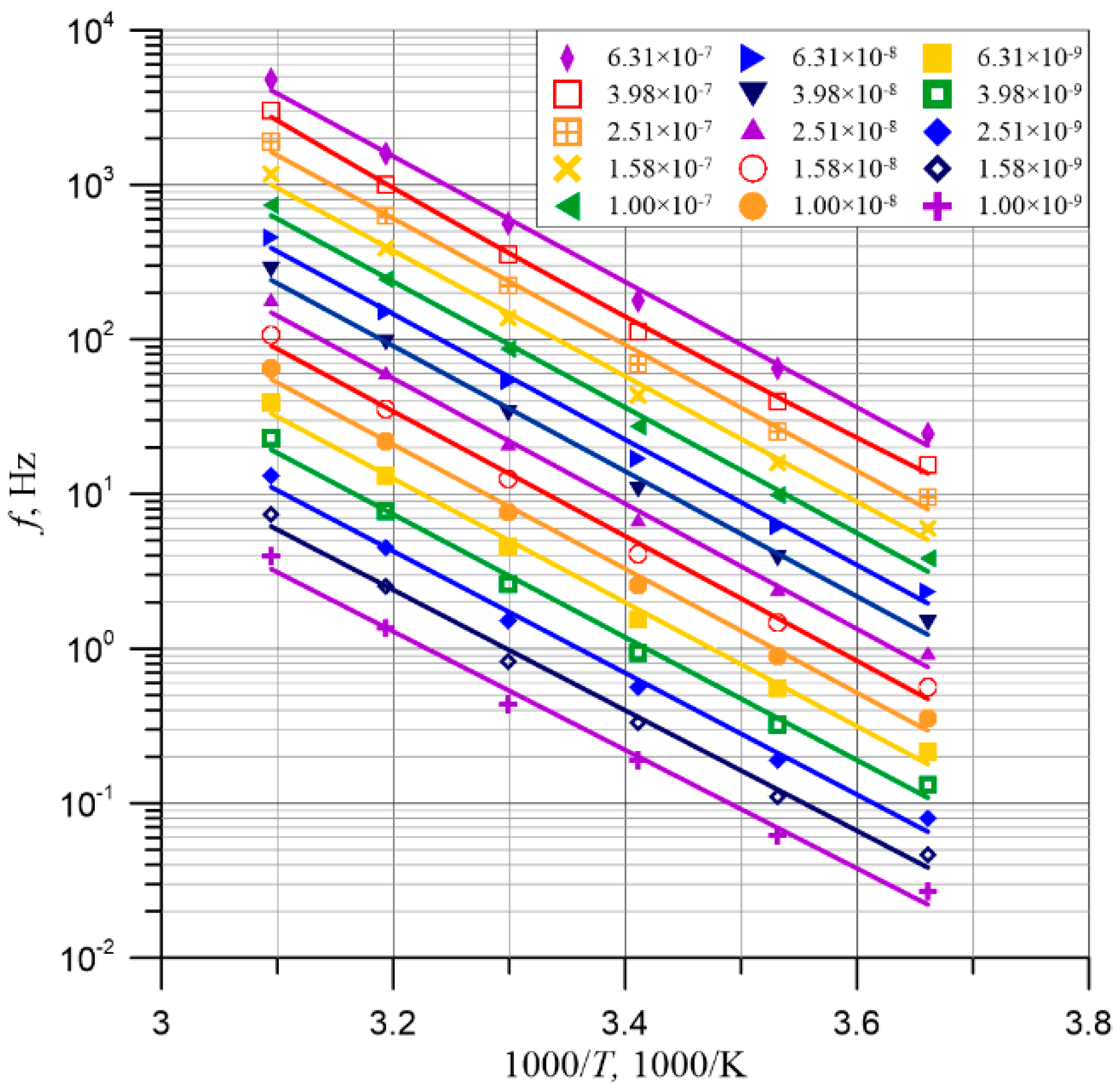
−7 S, marked with dashed horizontal lines. Similarly to the case described above, for the phase shift angle, a large number of shift angle values were selected in order to determine with high accuracy the mean activation energies for relaxation time in the admittance and the uncertainty of its measurements. The obtained frequency values were used to prepare Arrhenius’ diagrams, presented in
Figure 12. The linear approximation of Arrhenius’ diagrams, determined using the least squares method, proved their high accuracy since the determination coefficients R
2, calculated and presented in
Table 2, ranged from 0.988 and above. and their mean value was R
2 ≈ (0.990 ± 0.0009). On the basis of approximation formulas for each run in
Figure 12, the values of the activation energy for relaxation time in the admittance were determined, presented in
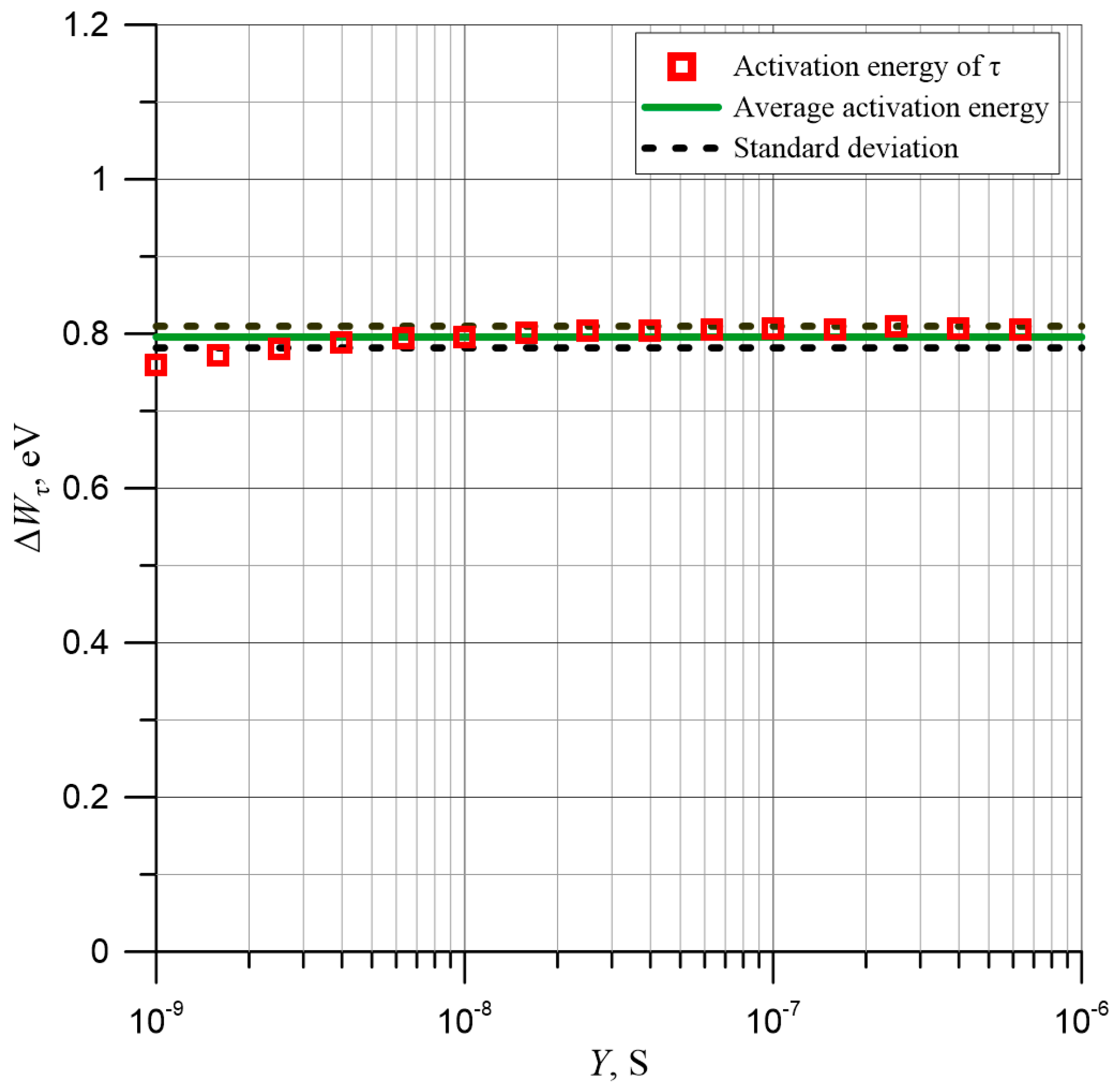
Table 2. The mean value of the activation energy for relaxation time in the admittance was Δ
Wτ ≈ (0.796 ± 0.0139) eV.
Figure 13 shows 15 values of the activation energy for relaxation time in the admittance for values between 10
−9 S and 6.31 × 10
−7 S. As can be seen, the activation energy for relaxation time in the admittance was a constant value over a wide range of admittance changes.
3.3. Determination of the Activation Energy of Admittance
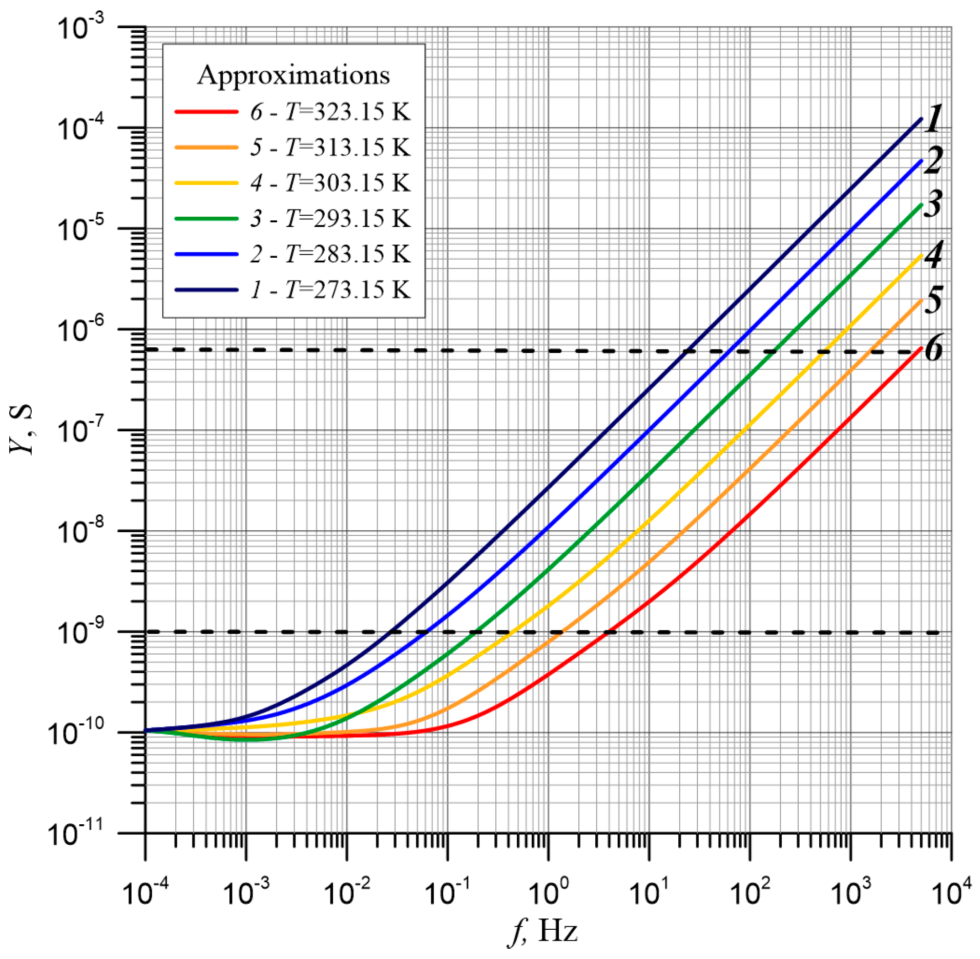
Once the activation energy for relaxation time in the admittance was obtained, its value was used to eliminate the effect of relaxation time on the frequency dependence of the admittance by shifting admittance curves along the X axis, as shown in
Figure 8. For this purpose, the waveforms for 273.15 K, 283.15 K, 303.15 K, 313.15 K, and 323.15 K have been converted to the reference temperature of 293.15 K using Δ
WY. The curves for 273.15 K and 283.15 K were shifted to a higher frequency area and for 303.15 K, 313.15 K, and 323.15 K to the lower frequency area (
Figure 14). The curves for frequencies above 5 × 10
−3 Hz were practically parallel. The values of all 6 shifted waveforms were in the frequency area from about 0.006 Hz to about 200 Hz, marked in
Figure 14 with dashed vertical lines.
As was described in the cases above, 15 points on the frequency axis were selected to calculate the activation energy for the relaxation time of the phase shift angle and the admittance in the frequency range 5 × 10
−3 Hz–200 Hz. This allowed for the accurate determination of the average value of activation energy in admittance and the uncertainty of its measurement. For each of these points, the admittance values occurring at different temperatures were determined. In total, 15 Arrhenius’ diagrams, shown in
Figure 15, were drawn up. For the experimental points, we performed a linear approximation of the functions by the least square’s method, shown in
Figure 15 as straight lines.
The quality of approximation was very high. The values of determination coefficients R
2, presented in
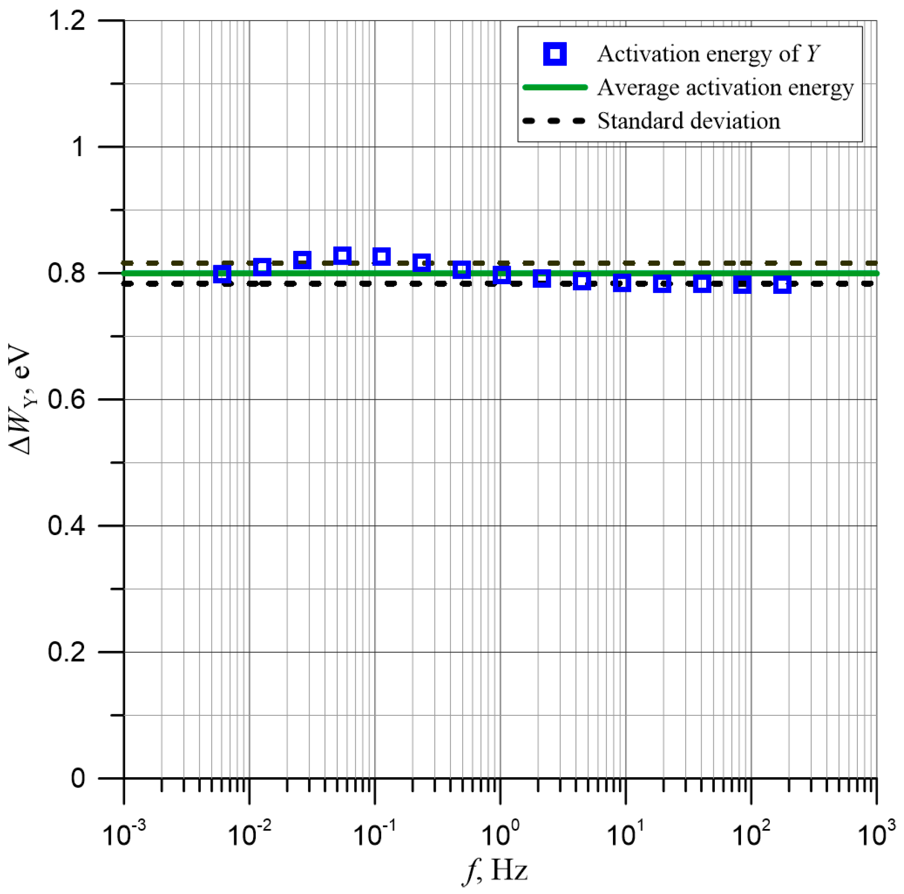
Table 2, were within 0.992 to 0.995, and their mean value was 0.994 ± 0.0009. Regarding the obtained approximation formulas, the values of activation energy in admittance (
Table 2) were determined for particular courses from
Figure 15. The average activation energy value of admittance obtained on this basis was ∆
WY ≈ (0.800 ± 0.0162) eV.
Figure 16 shows the frequency dependence of activation energy in admittance and the mean value ± standard deviation. The value of the activation energy in admittance was a constant value in a wide frequency range.
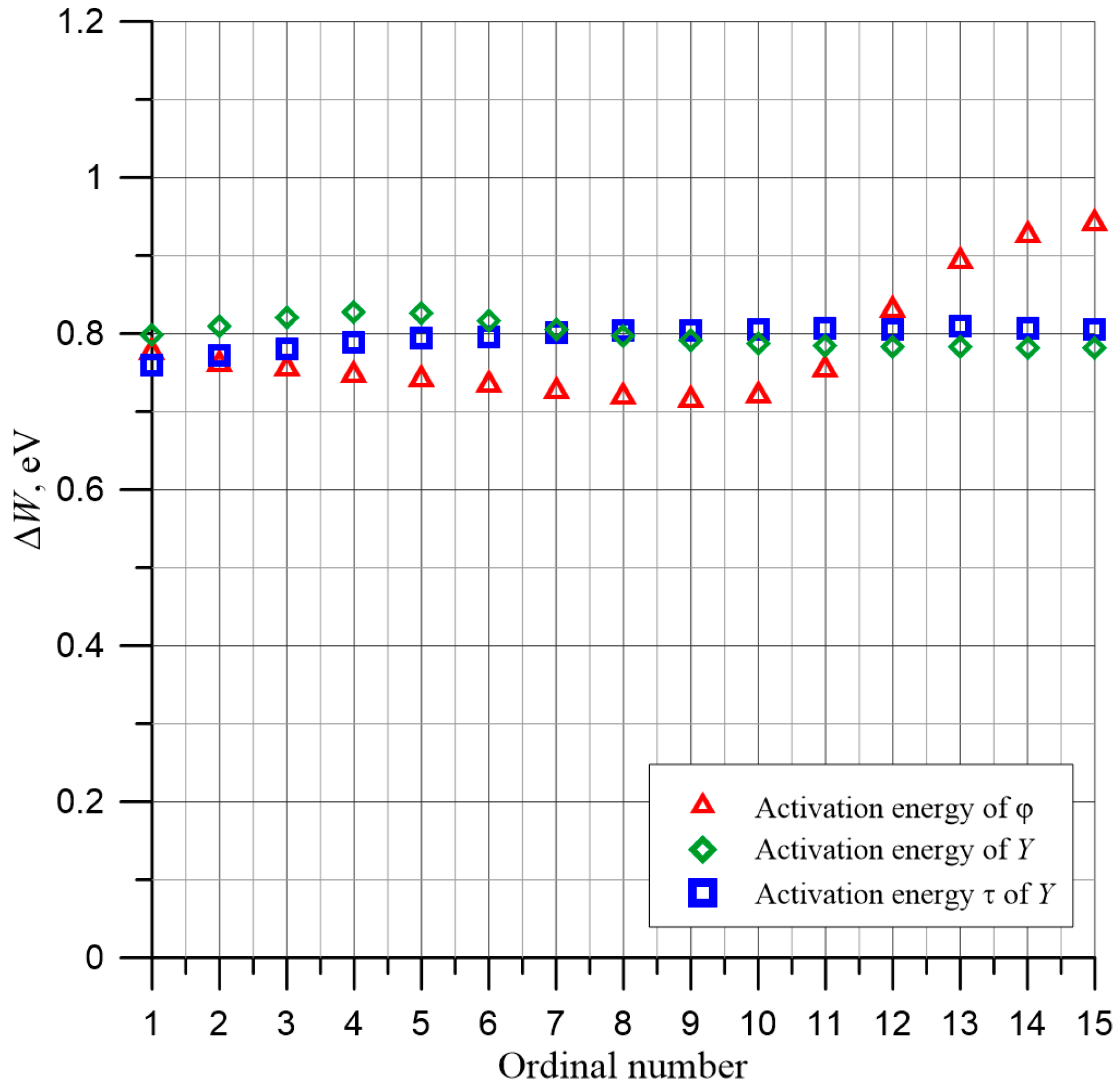
In total, 15 values for activation energy for relaxation time in the phase shift angle Δ
Wφ, activation energy for relaxation time in the admittance Δ
Wτ, and activation energy in admittance ∆
WY are specified above (
Table 2). A comparison of these values is shown in
Figure 17.
The mean value of activation energy for relaxation time in the phase shift angle was Δ
Wφ ≈ (0.783 ± 0.0744) eV, the activation energy for relaxation time in the admittance was Δ
Wτ ≈ (0.796 ± 0.0139) eV, and the activation energy of admittance was ∆
WY ≈ (0.800 ± 0.0162) eV. As can be seen, these values are close. The difference between the highest and lowest values was 0.017 eV. This was less than the standard deviation value (uncertainty of determination). This means that all three energy values describe different processes in cellulose composites, synthetic esters, and water nanoparticles, and are equal within the error limits. The mean value and standard deviation for the 45 residual activation energy values shown in
Table 2 was Δ
W ≈ (0.793 ± 0.0453) eV. From the comparison of this value with the activation energy value for alternating current conductivity (Δ
W ≈ 1.0582 eV [
27]) of the pressboard containing nanodrops of water and impregnated with transformer oil, it can be seen that the use of ester impregnation decreased activation energy by 0.26 eV. This was related to increased permittivity of esters compared to insulating oil.
The precise determination of activation energy opens up the possibility of converting the insulation parameters of transformers, which can be obtained at any operating temperature, into values at a reference temperature of 293.15 K (20 °C). This allows for the elimination of temperature influence on insulation parameters of transformers, as well as the separation of aging factors and other operating factors that may lead to deterioration.

 ,
, 


