Article

Variable Structure Control of a Small Ducted Wind Turbine in the Whole Wind Speed Range Using a Luenberger Observer

by
Diego Calabrese
,
Gioacchino Tricarico
,
Elia Brescia
*,
Giuseppe Leonardo Cascella
,
Vito Giuseppe Monopoli
and
Francesco Cupertino
Department of Electrical Engineering and Information Technology, Politecnico di Bari, 70126 Bari, Italy
*
Author to whom correspondence should be addressed.
Energies 2020, 13(18), 4647; https://doi.org/10.3390/en13184647
Submission received: 22 June 2020 / Revised: 31 August 2020 / Accepted: 4 September 2020 / Published: 7 September 2020

Abstract

:
This paper proposes a new variable structure control scheme for a variable-speed, fixed-pitch ducted wind turbine, equipped with an annular, brushless permanent-magnet synchronous generator, considering a back-to-back power converter topology. The purpose of this control scheme is to maximise the aerodynamic power over the entire wind speed range, considering the mechanical safety limits of the ducted wind turbine. The ideal power characteristics are achieved with the design of control laws aimed at performing the maximum power point tracking control in the low wind speeds region, and the constant speed, power, and torque control in the high wind speed region. The designed control laws utilize a Luenberger observer for the estimation of the aerodynamic torque and a shallow neural network for wind speed estimation. The effectiveness of the proposed method was verified through tests in a laboratory setup. Moreover, a comparison with other solutions from the literature allowed us to better evaluate the performances achieved and to highlight the originality of the proposed control scheme.

1. Introduction

In recent years, wind energy has been the fastest growing among renewable energy sources [1]. In particular, micro and small wind turbines are an attractive solution for distributed generation in urban areas, self-energy production, and microgrids [1,2,3,4,5,6,7,8,9,10,11]. Among these, variable-speed and fixed-pitch (VSFP) wind turbines are the most common because this configuration reduces the complexity and cost of the system [11,12,13,14,15,16]. Moreover, a direct-drive permanent magnet synchronous generator (PMSG) is usually equipped within this type of wind energy conversion system (WECS) because it avoids gearboxes, reduces costs, and increases reliability and efficiency [9,10,12,13,14].
Controlling a VSFP WECS under high wind speeds is a challenge. In fact, for these turbines, the pitch control cannot be applied for limiting the power and torque produced by the wind to avoid mechanical and electrical failure. To overcome this limitation, the most common approach used for VSFP WECS operations under high wind speeds is the soft stall method [11,14,15,16,17,18,19,20], which reduces the shaft speed to force the turbine to operate below its maximum efficiency. A control strategy alternative to the soft stall method is based on the flux weakening operation of an interior PMSG (IPMSG) connected to a full-bridge PWM rectifier [9,12,21]. This approach differs from the soft stall method, because it is based on operating the WECS at shaft speeds above the rated speed to reduce the power extracted from the wind. The soft stall method has been largely applied to WECSs with a power converter topology consisting of a passive diode rectifier and DC/DC converter [11,14,15,16,17,18,20]. However, very few studies have addressed control at high wind speeds of VSFP WECS with a PMSG, and a three-phase inverter-based back-to-back converter, in case the soft stall method is adopted. This solution, despite its higher costs, is characterised by higher efficiency ([1,22,23,24,25]) in comparison with the most commonly used topology for small-scale WECS, based on a 3-phase diode rectifier, a DC/DC converter, and a grid-connected three-phase inverter [1,6,11,13].
The operation of the WECS under high wind speeds is performed with a variety of specific aims and solutions, depending on its configuration and operating limits. In [9], the WECS was controlled to limit the generated electrical power to the rated power of the electrical generator. In [11], the machine-side boost converter voltage was limited to a safety value to prevent high wind speed from developing excessive torque at higher rotor speeds. In [12,26], for wind speeds above the rated speed, the IPMSG was controlled to maximise the electrical power generated by considering the current and voltage constraints. In [14,20], after constant-speed stall control, a constant aerodynamic power soft stall control was performed to avoid exceeding the rated power of the turbine. In [15,18], after the constant-speed stall operation, the control strategy limited the generated DC power considering the electrical operating limits of the system. In [17], the rated electrical torque, which occurs when the boost converter operates at its rated current, was held until the maximum wind speed at which the generator can counteract the aerodynamic torque was reached. To the best of the authors’ knowledge, the VSFP WECS was operated with respect to the rated aerodynamic power of the wind turbine at high wind speeds only in [14,20]. In these studies, the proposed control strategies performed constant aerodynamic power soft stall control. During this operation, the shaft speed decreased while the aerodynamic torque increased to maintain constant aerodynamic power. With increasing wind speed, this operation can lead to the development of excessive aerodynamic torque and damage the wind turbine. However, these two studies did not consider the issue of limiting the aerodynamic torque for safety reasons.
The use of aerodynamic power or torque observers to perform constant aerodynamic power or torque operation is crucial [14,20]. In the literature, different aerodynamic torque observers (ATOs) have been proposed. In [23,24,25], the aerodynamic torque is estimated by using a sliding-mode observer. A new high-gain robust ATO is proposed in [9]. In [14,17], a simple adaptive observer based on an approximated equation of rotational mass equilibrium is proposed. A Luenberger observer (LO) was proposed in [26,27], but these works lack experimental validation. The advantages of using an LO are the ease in modelling operations and the easy way of achieving a fast convergence.
In this paper, we propose an original control strategy for a small VSFP ducted horizontal axis wind turbine (DHAWT) equipped with a full-embedded annular brushless PMSG (ABPMSG). The ABPMSG is grid-connected through a back-to-back connection of two three-phase inverters. A tripartite control scheme based on the soft stall method is proposed for the DHAWT operation under high wind speeds. This operating range is subdivided into constant shaft speed, constant aerodynamic power, and constant aerodynamic torque subregions. To perform this control strategy, a variable structure controller (VSC) combined with an aerodynamic torque LO and a neural network (NN) wind speed estimator (WSE) was designed. This control scheme maximises the power extracted from the wind, which is compatible with the mechanical safety limits of the DHAWT—the rated shaft speed, rated aerodynamic power, and maximum aerodynamic torque. Therefore, the contributions of this study are as follows: the achievement of the soft stall method with a back-to-back power converter topology, the operation of the wind turbine once the aerodynamic torque limit is reached, and the experimental validation of a discretised LO.
Experimental tests were conducted in a laboratory setup emulating a ramp wind speed pattern to prove the effectiveness of the proposed control scheme. In the literature, there is no uniformity in the wind speed pattern used for the emulative experimental tests of WECS. The actual measured wind speed patterns were used from [12,28], while irregular artificial wind patterns have been adopted from [14,18,25,29]. Such wind speed patterns allow for analysis of the dynamic performances of the proposed control strategies. However, the use of wind speed patterns with multiple steps ([11,13,15,16,17,30,31,32]) and single steps or constant speeds ([10,33,34,35]) allows for analysis of the effectiveness of the control scheme in specific wind speed subregions. In this study, a ramp wind pattern was chosen to show the fitting of the actual aerodynamic power and torque with the ideal regulation characteristics over the entire wind speed range. However, the examination of the dynamic performances of the proposed control scheme was not the purpose of this work.
The paper is organised as follows: In Section 2 a description of the WECS is provided; in Section 3 the proposed variable structure controller is described and analysed in detail. In Section 4 the experimental results are shown, accompanied by a quick illustration of the test rig. Finally, conclusions are presented in Section 5.

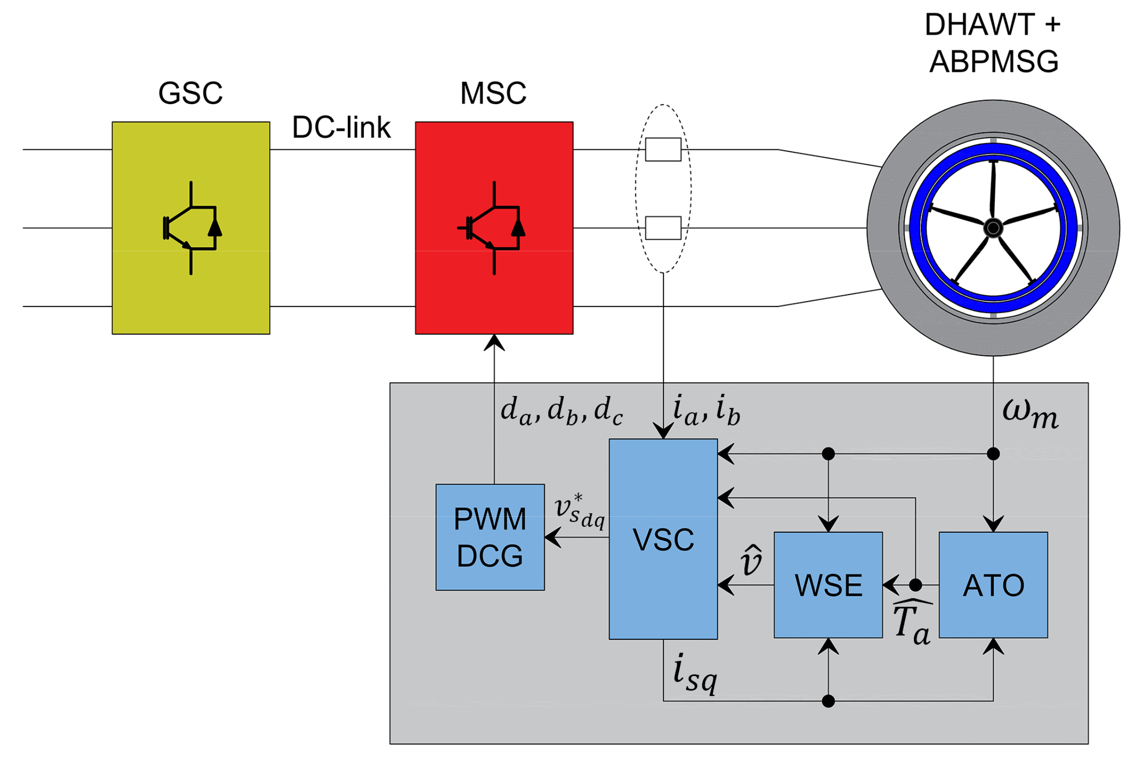
2. System Description

In this section, an overview of the proposed WECS is provided to contextualise the entire work. The system is composed of a DHAWT, an ABPMSG, and a back-to-back power converter topology, as shown in Figure 1.

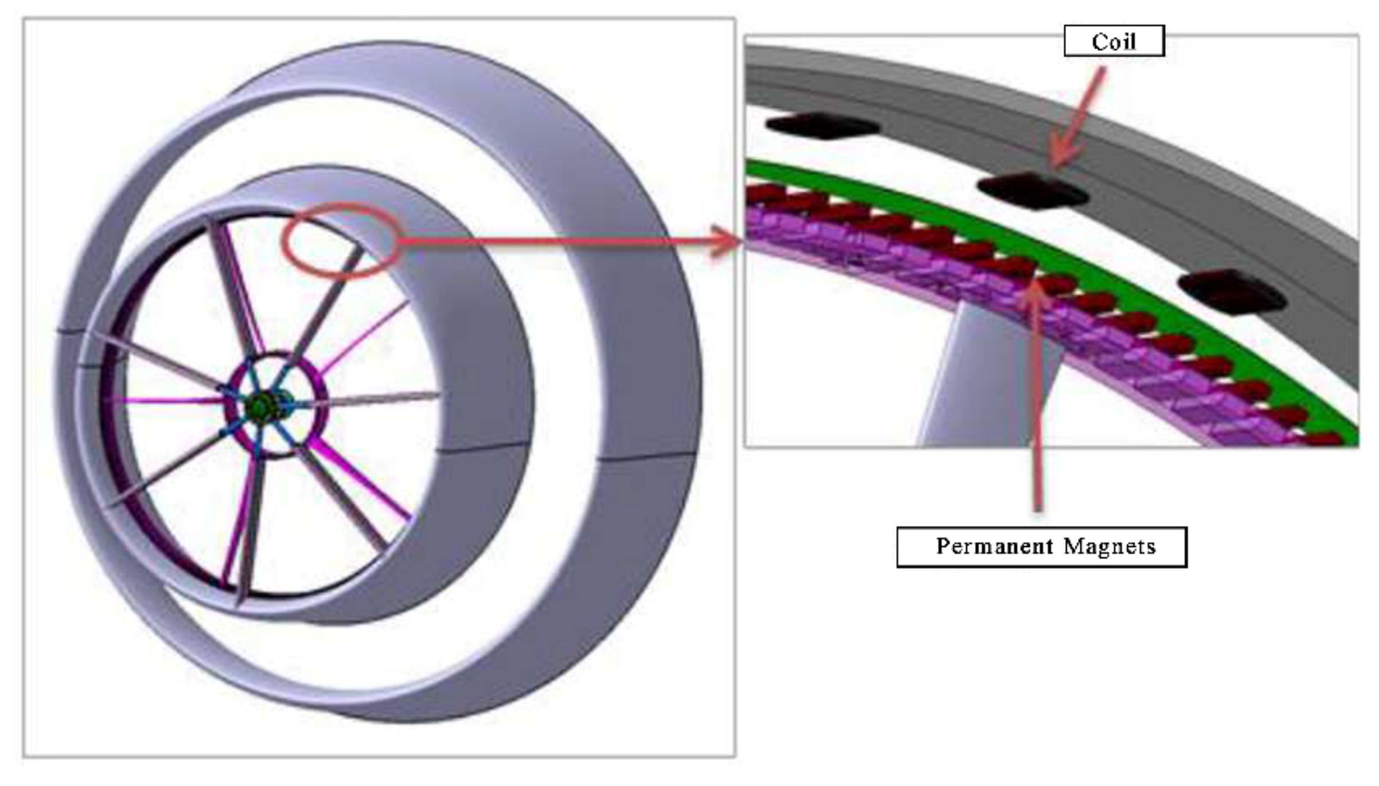
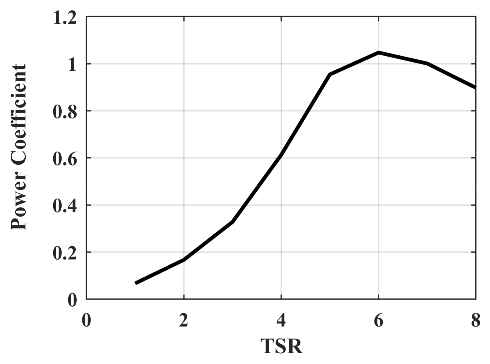
2.1. Ducted Wind Turbine

The DHAWT is shown in Figure 2. In these wind turbines, a divergent duct increases the pressure drop across the disk of the rotor. This increases the power production compared to conventional wind turbines [8,36]. The DHAWTs’ performance enhancements allow for reduction in rotor diameters at equal rated power, favouring rotor rigidity and reducing blade deformations. Moreover, the adoption of a diffuser reduces the cut-in speed and wind noise compared to conventional ones [37,38]. In Table 1, the most relevant parameters of the DHAWT are considered in this work, which corresponds to the one in [37]. It can be noted that the optimal power coefficient C p m a x , due to the presence of the diffuser, is characterised by a higher value than that of conventional wind turbines, whose theoretical maximum value, according to Betz’s theory, is 16 / 27 . In the literature, it has been demonstrated that for DHAWTs, this coefficient can overcome the value of 1 [37,38,39]. To obtain the DHAWT characteristic curve, which expresses the relationship between the power coefficient and the tip-speed ratio (TSR), in [37] a non-conventional approach was used. The flow interacting with the DHAWT was computed using computational fluid dynamics (CFD) simulations. Source terms for the momentum equations were introduced inside the domain swept by the rotor to take the turbine effect on the flow field into account. From the CFD simulation, it is possible to compute the local relative velocity, and from the polar characteristics of the aerodynamic blade profile (with an approach similar to the blade element theory (BEM)), it is possible to compute the force coefficient to determine the force exchange between the flow and the rotor. Using CFD simulations has improved the computational accuracy of the entire flow field, and hence the computation of the turbine performance. The obtained DHAWT characteristic curve is shown in Figure 3.
Regarding the equations used in the model, the aerodynamic reference power used to evaluate the turbine performance is expressed by the following equation:
P w = 1 2   ρ   A   v 3    
where ρ is the air density, A is the rotor swept area, and v is the unconstrained wind speed. The aerodynamic power caught by the wind turbine is related to P w through the power coefficient C p :
P a = C p λ   P w
This coefficient denotes the power conversion efficiency of the wind turbine, which depends on the TSR λ , defined by
λ =   ω m   R v    
where R is the blade tip radius and ω m is the shaft speed. Replacing (1) in (2), the following expression of P a is obtained:
P a = 1 2   ρ   π   R 2   C p λ v 3
The expression of the aerodynamic torque T a is obtained by the division between P a and shaft speed ω m :
T a = 1 2   ρ   π   R 2   C p λ   v 3 ω m
By replacing ω m in (5) through (3), a new expression for T a is achieved:
T a = 1 2   ρ   π   R 3   C p λ   v 2 λ
Fore more information see Supplementary Materials.

2.2. Annular Brushless PMSG

An innovative full-embedded ABPMSG is considered. This generator was designed in agreement with the method presented in [8]. The purpose of this method is to design a PMSG integrated with a DHAWT, to achieve a target torque with a multi-objective optimisation aimed at minimising the weight of the permanent magnets and copper. The ABPMSG rotor consists of a fibreglass ring with internal permanent magnets. It is directly connected to the blade tips and is concentric to a segmented iron stator, which is instead embedded on the diffuser (Figure 2). Concerning the stator windings, coils are realised on multi-layer printed circuit boards and are wye connected. This solution makes the manufacturing and assembly process easier. In Table 2 all parameters of the ABPMSG are summarised.
Regarding the mathematical model, Park transformation was performed to characterise the three-phase machine in the d-q reference system.
v s d = R s i s d + L s d i s d d t n p ω m L s i s q
v s q = R s i s q + L s d i s q d t + n p ω m L s i s d + n p ω m ψ P M
The previous equations state a relationship between the axis voltages ( v s d , v s q ) , the d–q axis currents, i s d ,   i s q ) , and the shaft speed ( ω m ) . The parameters are the phase resistance R s , stator inductance L s , rotor flux linkage ψ P M , and number of pole pairs n p . The electromagnetic torque ( T g ) depends on the q-axis current, number of pole pairs, and rotor flux linkage:
T g = 3 2   n p ψ P M i s q = K c i s q
K c is the torque constant. The expression above shows a torque consisting of a single contribution, that is, the magnetic field alignment torque. In fact, PMSGs with internal rotor magnets have an additional torque contribution; that is reluctance torque. This contribution is missing in the model because the ironless rotor can be considered isotropic, like that of a superficial PMSG (SPMSG). This is also the reason why the d-axis inductance and q-axis inductance are the same. The considered model is completed by a third equation, which expresses the rotational mass equilibrium:
T a T g T a v ω m = J   d ω m d t
where T a is the aerodynamic torque, T a v represents the dynamic friction loss torque, and J is the total inertia momentum of the wind turbine.

2.3. Power Conversion Stage

The power conversion stage consists of two power converters in a back-to-back configuration. The ABPMSG is directly coupled to a machine side converter (MSC), which is connected to a grid side converter (GSC). The MSC is a three-phase full-bridge PWM rectifier whose duty cycles are provided by the proposed control scheme to perform a field oriented control (FOC). The GSC is a PWM inverter that maintains a constant voltage on the DC-link v D C , and synchronises and controls the output voltages and currents to establish a correct grid connection. Thus, the GSC leads to grid frequency decoupling and transfers the generated power from the DC link to the grid.

3. Control Scheme Description

The WECS control scheme shown in Figure 1 can be gathered in four macro-blocks: the VSC, the ATO, the WSE, and the PWM blocks. The sensors present in the scheme are the phase current sensors and an optical encoder for the measurement of ω m .

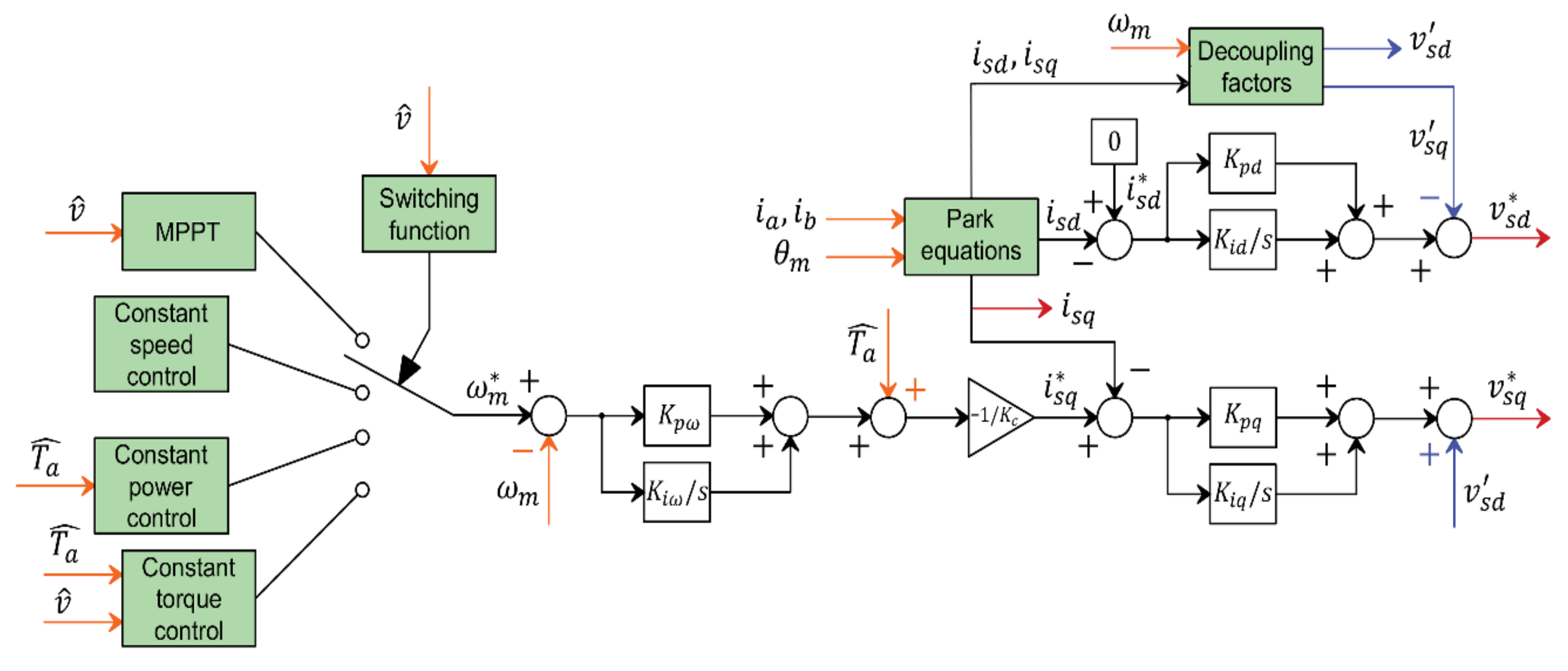
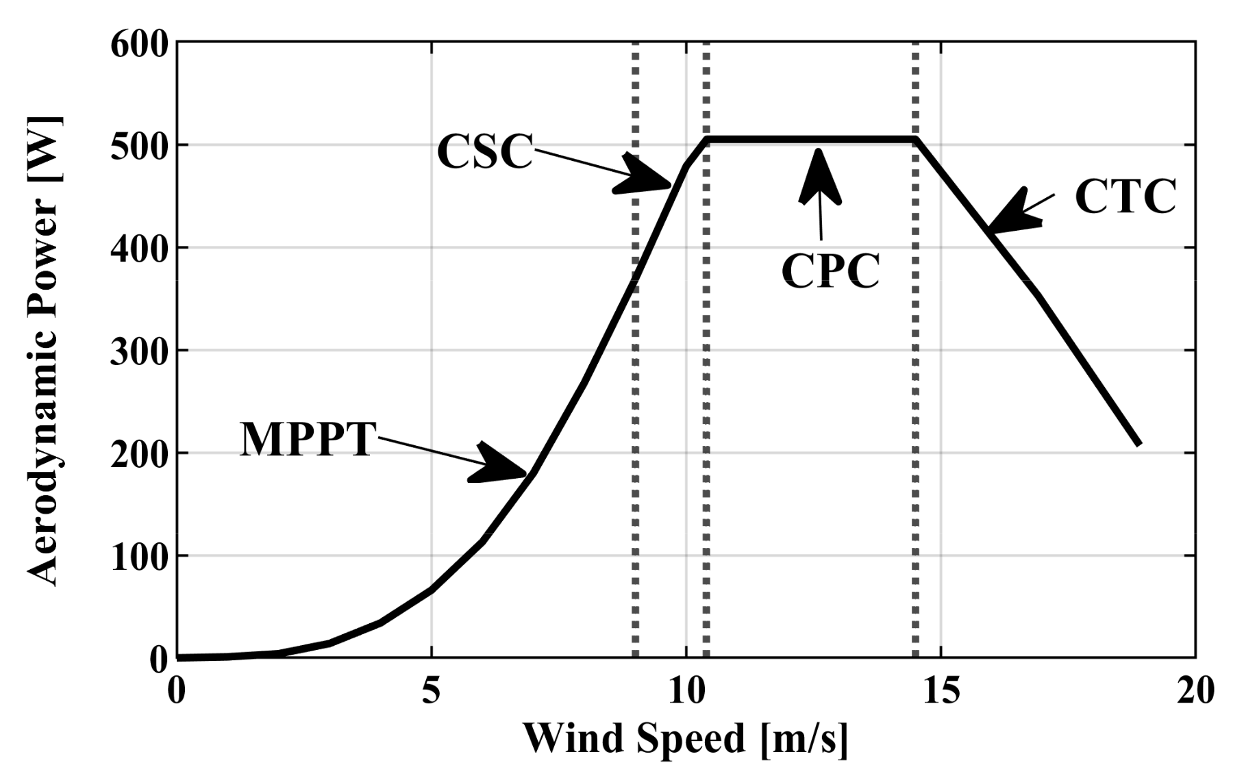
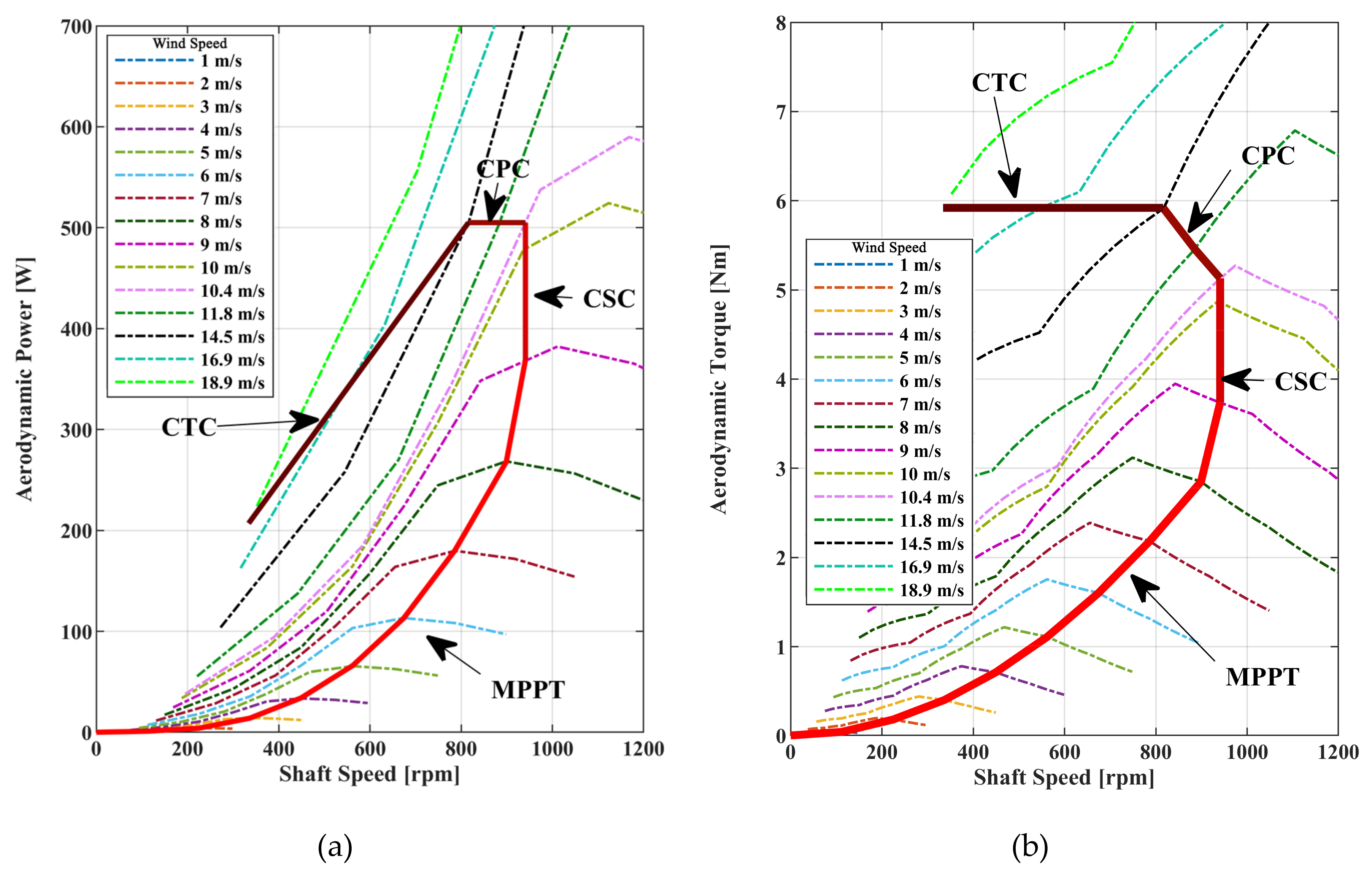
3.1. Variable Structure Controller

The VSC is shown in Figure 4. In this scheme, all the symbols under “^“ represent estimated variables, while the symbols marked with “*” denote reference variables. This scheme realises a cascading speed-current FOC. A commonly adopted solution for the FOC is based on the use of proportional-integral (PI) controllers for speed and current regulation. This solution is simple and robust, and its effectiveness for the control of WECS with a PMSG and a three-phase full-bridge PWM rectifier MSC has already been demonstrated [24,29,40]. The speed controller is a PI regulator with feedforward for the aerodynamic torque disturbance rejection, while the current controllers are simple PI regulators. Therefore, K p ω , K i ω , K p d , K i d , K p q , and K i q represent the PI gains of the speed and current control loops, respectively. The q-axis current loop performs torque regulation while the d-axis loop performs maximum torque per ampere (MTPA) control. The “decoupling factors” block operates the d and q-axis decoupling as follows:
v s q = n p ω m L s i s q
v s d = n p ω m L s i s d
The “Park equations” block operates the Park transform using the phase currents i a and i b and the rotor position θ m .
The shaft speed reference ω m * is provided by four different laws to achieve maximum power point tracking (MPPT) control, constant speed control (CSC), constant power control (CPC), and constant torque control (CTC) in four different wind subregions. The shaft speed reference law is selected by the switching function according to the estimated wind speed value. The aim of the control scheme is to achieve the ideal aerodynamic power curve over the entire wind speed range shown in Figure 5. This curve shows the maximum aerodynamic power that can be extracted for a given wind speed, ensuring the respect of the mechanical limits for safe operation of the DHAWT (i.e., rated speed and power and maximum aerodynamic torque). The four control laws and the corresponding wind subregions are summarised in Table 3 while Table 4 shows the wind speed threshold values.

3.1.1. Maximum Power-Point Tracking

The MPPT is performed if the wind speed is between the cut-in speed v c i and the wind speed which corresponds to the rated shaft speed v s p d (i.e., the low wind speed region). The aim of the MPPT is to extract the maximum available aerodynamic power for a given wind speed. In the literature, several MPPT methods for VSFP WECS have been proposed. The first approach is to consider the fluid dynamic model of the wind turbine to provide optimal references for the shaft speed ([11,17,29,30,33,41]), or torque ([9,12,31]), and power ([14,18,34]). These approaches have the advantage of being fast and stable, but are affected by inaccuracies due to production tolerances, model and parameter uncertainties, and time variance. Moreover, these methods generally require the measurement of wind, shaft speed and torque. To avoid the use of mechanical sensors, many sensorless algorithms have been proposed in previous studies to achieve MPPT. For a WECS with a diode rectifier and boost converter, the proposed solution is based on tracking the optimal boost converter voltage on the rectifier side using only voltage and current sensors [11,14,33,34]. Others are based on the use of observers and estimators of shaft ([17,29,42,43]), wind speed ([26,29,32,40,41,44]), and aerodynamic torque ([9,14,17,23,24,25,26,27]). A robust and parameter-independent approach is based on the perturb and observe (P&O) concept that is widely treated in the literature in its many variants [10,13,14,15,16,18,28,45,46,47]. This approach avoids the use of mechanical sensors and does not require prior knowledge of the WECS because the optimal rotor speed is achieved with a research algorithm performed during the operation of the wind turbine. However, this approach is slower than the first one for tracking the optimal speed, and its accuracy depends on the step size of the P&O algorithm. Finally, an innovative and robust approach was proposed in [35] in which a neural network (NN) was used to determine the reference shaft speed that maximises power extraction. However, this method requires a period of operation in which the NN has to be trained.
In this study, we use an approach based on the model of a wind turbine combined with an NN WSE. During the MPPT, ω m * is provided by a look-up table (LUT), whose input is the estimated wind speed, to maintain the TSR at its optimal value as the wind speed changes. The optimal value of the TSR is the one that maximises C p ; therefore, it maximises the extracted wind power, according to (2). This is the well-known optimal tip-speed ratio method. The LUT used for the MPPT control is based on the curve depicted in Figure 6a, which is built considering the model of the DHAWT.

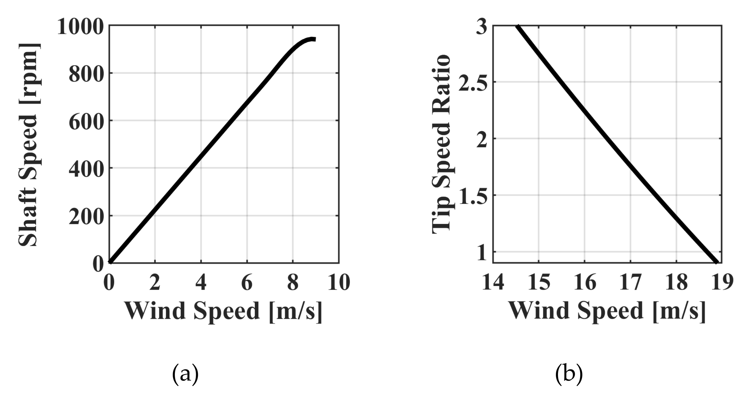
3.1.2. Operation in the High-Wind Speeds Regions

The CSC is performed for wind speeds above v s p d and below the rated speed v r a t e d . Once the rated shaft speed is reached, this should be kept constant to ensure the respect of the speed limit of the DHAWT, and to extract the maximum available power. Therefore, the control law is
ω m * = ω r a t e d
By maintaining the shaft speed, the increase in wind speed will increase aerodynamic power, as shown by the ideal regulation characteristic shown in Figure 7a. Therefore, the law expressed by (13) is performed until the rated aerodynamic power ( P r a t e d ) is reached.
The CPC is performed for wind speeds above v r a t e d and below v t r q , which is the speed at which the maximum torque is reached. For these wind speeds, a soft stall is performed to limit the aerodynamic power according to the following law:
ω m * = P r a t e d T ^ a
where T ^ a is the estimated aerodynamic torque. While this control law is applied, the shaft speed decreases while the aerodynamic torque T a increases, keeping the power constant until the torque limit of the DHAWT is reached, as depicted by the ideal regulation characteristics shown in Figure 7a,b.
The maximum aerodynamic torque is reached when the wind speed equals v t r q . CTC is performed from this wind speed until the cut-out speed. In this case, the shaft speed reference is
ω m * = T m a x   ω * T ^ a
where ω * is:
ω * = λ * L U T v   v R
in which λ * L U T v is computed by an LUT based on the curve depicted in Figure 6b. This curve expresses the TSR value that ensures the operation of the DHAWT at the maximum torque as the wind speed changes in the CTC subregion. The ideal power and torque regulation characteristics corresponding to the four control laws described above are illustrated along the fluid dynamic characteristics of the DHAWT in Figure 7a,b.

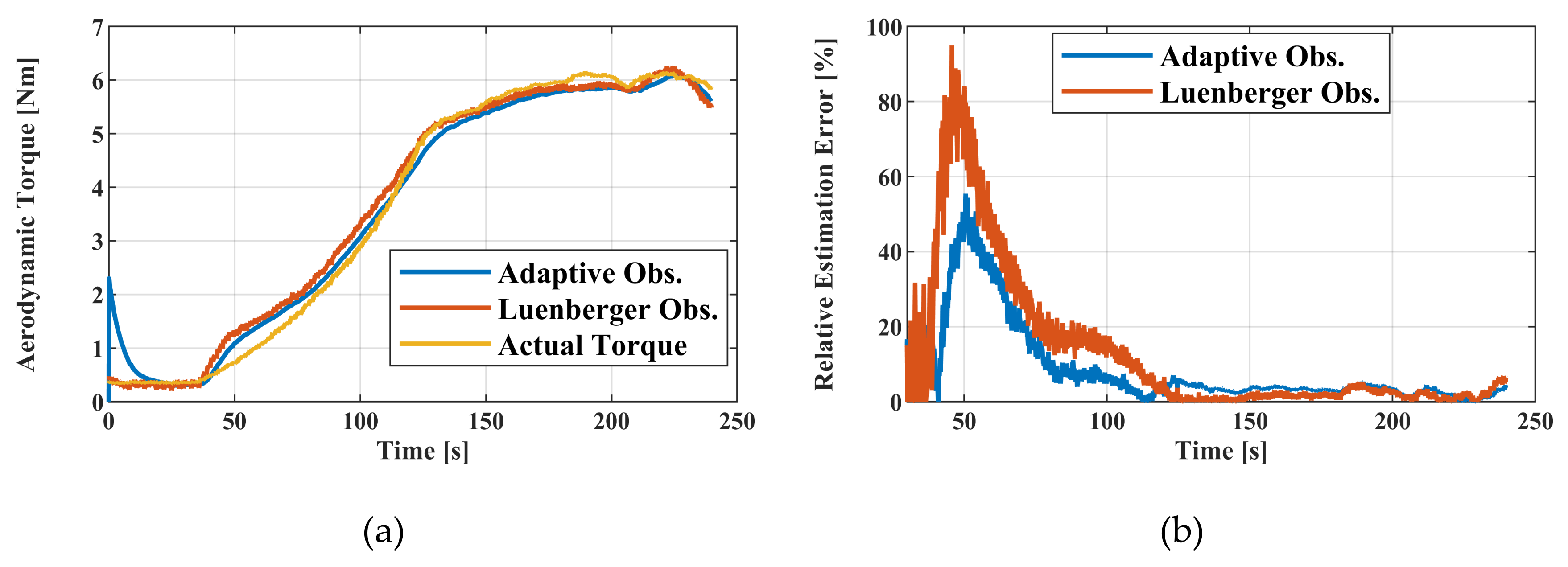
3.2. Aerodynamic Torque Observer

To estimate the aerodynamic torque, an LO was adopted. The LO is based on the following linear time-invariant continuous-time reference model:
x ˙ = A x + B u y = C x
where:
x = ω m T a ,   u = i s q ,   A = 0 1 J 0 0 ,   B = K c J 0 ,   C = 1 0
This model has been defined considering (10) and by introducing T a as an exogenous variable, with the following assumptions:
  • The dynamic friction losses are negligible ( T a v = 0 ) ;
  • The derivative of the aerodynamic torque is zero ( T ˙ a = 0 ) .
In this model, x and y are the state and measurable outputs of the system, respectively, while u is the input of the system. The LO is described by the following equations:
x ^ ˙ = A ^ x ^ + B ^ u + L y y ^ = C x ^
where x ^ and y ^ are the estimations of x and y , respectively; A ^ , B ^ and L are designed to make the estimation error asymptotically converge to zero:
e = x x ^
By defining A ^ and B ^ as follows:
A ^ = A L C
B ^ = B
and by substituting into (18) we obtain
x ^ ˙ = A x ^ + B u + L y C x ^
Considering (17) and (22), the differential error can be written as
e ˙ = x ˙ x ^ ˙ = A e L C e = A L C e
For the error e to asymptotically converge to zero, the matrix L should be designed to obtain eigenvalues of the matrix A L C with a negative real part.
To apply the Luenberger method, the system considered should be observable.
Lemma 1.
An LTI system is observable if and only if the rank of the observability test matrix (OTM) is equal to the system dimension n.
For an LTI model described by (17), the OTM is
O = C C A C A 2 C A n 1
In this case, the system dimension is 2, and the actual expression of the OTM is
O = 1 0 0 1 J
The determinant of the OTM determinant is 1 / J , so the condition of 0 is satisfied.
In this study, we experimentally evaluated the performance of a discretized version of the LO, as reported in Appendix B. Moreover, to better evaluate these performances, a comparison with the aerodynamic torque observer proposed in [17], whose effectiveness has been already proven with experimental tests, has been made. The observer proposed in this paper consists of a closed shaft speed loop with a proportional regulator that forces the output of this system to converge to the estimated shaft speed that is used as the reference. Moreover, this observer uses the estimated torque of the PMSG as the input. We have chosen properly to compare the LO observer with this adaptive observer because both require knowledge of the shaft speed, PMSG torque, and system inertia, and because both do not consider dynamic friction losses. In this work, we used the measured shaft speed and the estimated ABPMSG torque as the reference and the input of the observer used in [17]. The estimated ABPMSG torque is obtained by the product of the measured q-axis current and torque constant.

3.3. PWM

The d-q voltage references v s d * and v s q * provided by the PI current regulators are transformed in the three-phase voltage references v s a * ,   v s b * ,   v s c * by using the Park anti-transformation. These references are used to compute the duty cycles for each leg of the MSC:
d a = v s a * v D C + 0.5 d b = v s b * v D C + 0.5 d c = v s c * v D C + 0.5

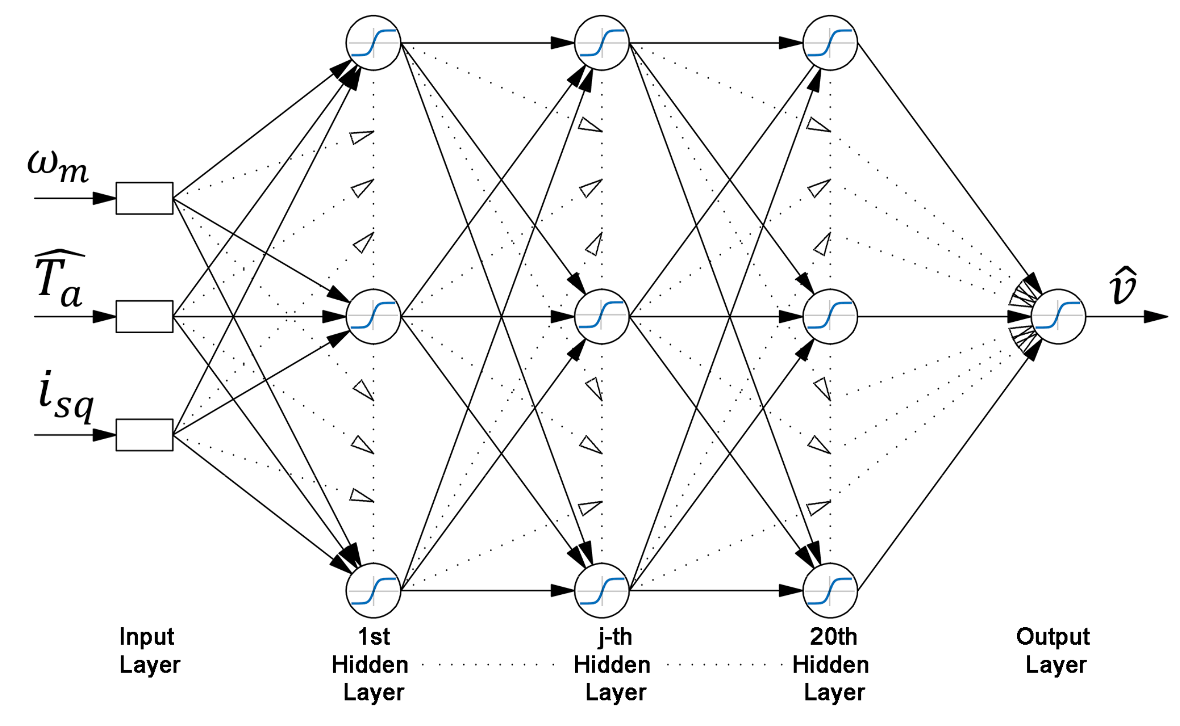
3.4. Wind Speed Estimation

The proposed control scheme needs real-time wind speed for the transition between the four control laws, and to calculate the shaft speed reference during the MPPT control and CTC. Determining a strategy to estimate the wind speed can be beneficial, instead of using an anemometer, to reduce costs, complexity, and the failure rate of the system [19,22,28,30]. In the literature, different approaches have been proposed for wind speed estimation. In [32,41], the method used is based on calculating the wind speed using the inverse model of the wind turbine, and the estimation of the aerodynamic torque and shaft speed. A similar approach was used in [40], wherein the estimated aerodynamic power was used instead of the aerodynamic torque. These model-based methods can be imprecise because of estimation errors of the aerodynamic torque, aerodynamic power, and shaft speed, and because of uncertainties in the wind turbine model. In [44], a support vector machine was used to predict the wind speed. The model was trained to track the wind speed measured by an accurate radar anemometer during a short initial period of the operation of the WECS. In [26,29], a three-layer neural network is proposed, whose inputs are the estimated shaft speed and aerodynamic torque/power. The machine learning methods can ensure better results in comparison with those based on the inverse model of the wind turbines but require a training phase in which the wind speed should be measured. However, as suggested in [44], once the training phase is over, the sensor used for the wind speed measurement can be used for the training with other wind turbines.
In this paper, we propose a WSE consisting of a shallow NN whose inputs are the estimated aerodynamic torque, the measured shaft speed, and the q-axis current of the ABPMSG. To demonstrate the superiority of this approach over the model-based WSE, their performances will be compared with experimental tests.

3.4.1. Shallow NN WSE

As shown in Figure 8, the WSE consists of an NN whose inputs are, T a ^ , ω m , and i s q . This is a shallow NN with twenty hidden layers, each comprising 10 neurones. The activation function of each neurone is a hyperbolic tangent sigmoid (tansig), whose mathematical representation is stated by the following equation:
t a n s i g n = 2 1 + e 2 n 1
Each neurone is characterised by biases and weights, which are the coefficients of the NN that should be determined with the training process. Appendix A demonstrates that the wind speed cannot be expressed as a function of T a ^ and ω m due to the presence of aerodynamic torque estimation errors. Instead, as will be demonstrated in Appendix A, there exists a function f v such as
v = f v T a ^ , ω m ,   i s q
Thus, the proposed NN can be effectively used to approximate this function.
In a real WECS, this NN should be trained by using the values of the input and output variables registered during a test period in which the WECS is driven by using the proposed control scheme in the whole wind speed range and an anemometer for the wind speed measurement. However, in this study, instead of using an anemometer on a real DHAWT, the training data were generated with an experimental test on the test rig described in Section 4. This test was performed by emulating the system described in Section 2 and Section 3 with a predefined wind speed pattern. The chosen wind speed pattern for the training data generation consists of a uniformly random noise signal that overlaps with a ramp that covers the entire wind speed range of the DHAWT. In this way, the values of the wind speed are known because the wind speed pattern is predefined while the inputs of the shallow NN are based on real measurements performed during the test.
The dataset obtained during the experimental test is approximately 2.3 × 10⁶ samples. However, this experimental dataset was downsampled by a factor of 10 and randomly split into training data, validation data, and test data. These datasets are made up of 70%, 15%, and 15% of the samples of the whole downsampled experimental dataset. The training dataset is used for determining the weights and biases of the NN to reduce the error between the output of the NN and the wind speed values of the training dataset. To avoid overfitting of the NN, the stop criterion adopted for the training process is based on the maximum validation failures. In this way, the training process stops when the number of consecutive training epochs for which the estimation error of the validation data (generalisation error) increases is equal to six. The test dataset is used as an additional verification of the training performance. The Levenberg–Marquardt (LM) algorithm is used to train the NN. This algorithm is known as one of the most efficient training algorithms for small and median size patterns. However, LM implementations require a large amount of available memory because the algorithm is based on the calculation of a Jacobian matrix whose size is proportional to the number of training patterns [48,49]. In this specific application, the LM algorithm was a good choice to train the NN quickly.
While the number of neurones per layer was chosen a priori, the number of hidden layers was chosen with the trial and error process. Eleven NNs were trained with an increasing number of hidden layers up to 22 hidden layers. The best trained NN was the one with twenty hidden layers with mean squared errors on the training, validation, and test datasets, respectively, of 1.348 × 10⁻³, 1.356 × 10⁻³, and 1.345 × 10⁻³, respectively.

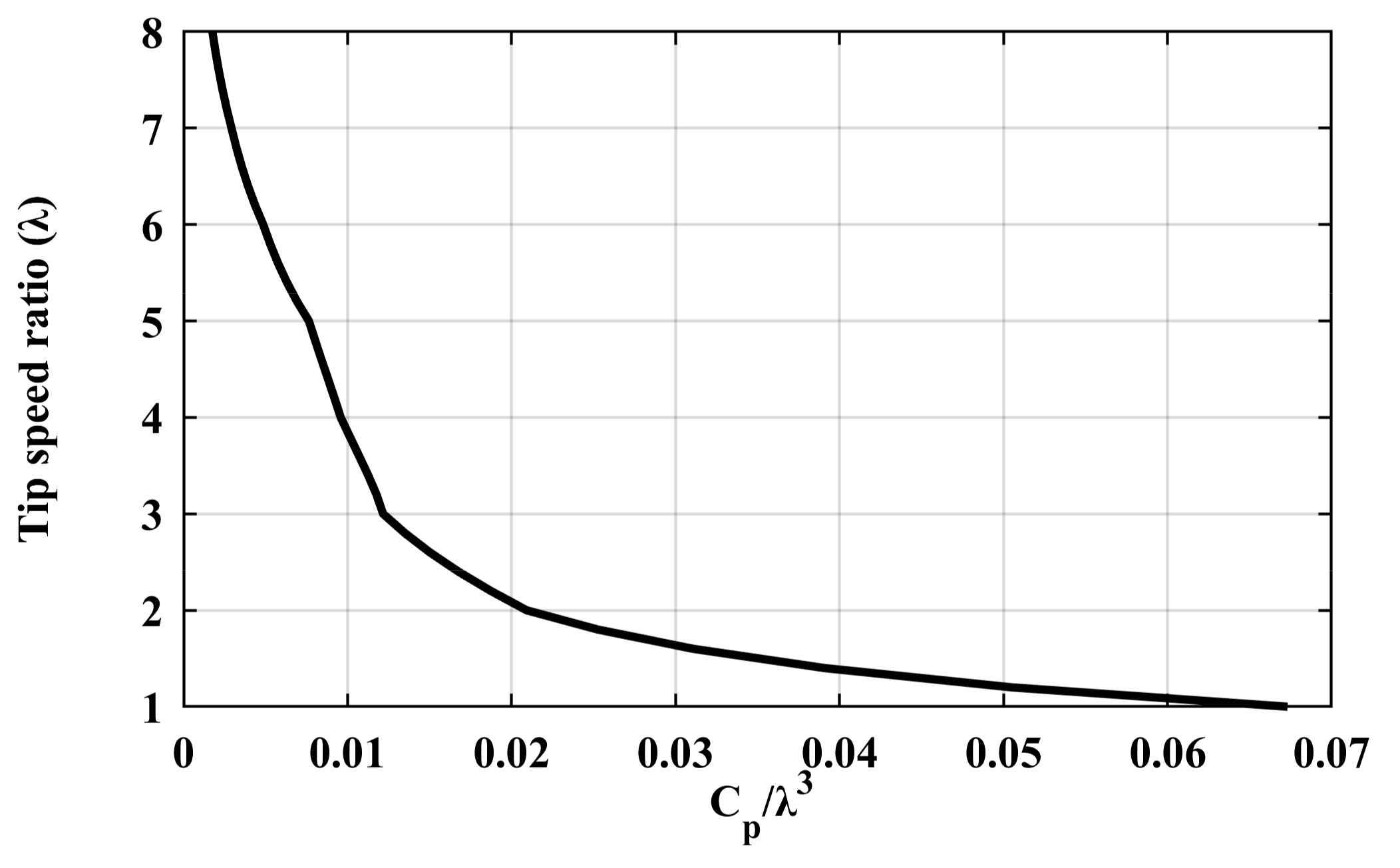
3.4.2. Model-based WSE

The model-based approach used in [32,41] makes use of the inverse model of the wind turbine. By using (3) and (5) is possible to highlight a relationship between, T a , ω m and λ :
T a = 1 2   ρ   π   R 5   C p λ λ 3 ω m 2
This equation can be rearranged as follows:
C p λ λ 3 = T a 1 2   ρ   π   R 5   ω m 2
The term C p λ / λ 3 can be computed from (30) by using T a ^ instead of, T a and the measured shaft speed ω m . Thus, λ can be determined by exploiting the relationship C p λ / λ 3 λ , as shown in Figure 9, for the current DHAWT. Finally, the estimated wind speed is calculated by reversing (3).

4. Experimental Results

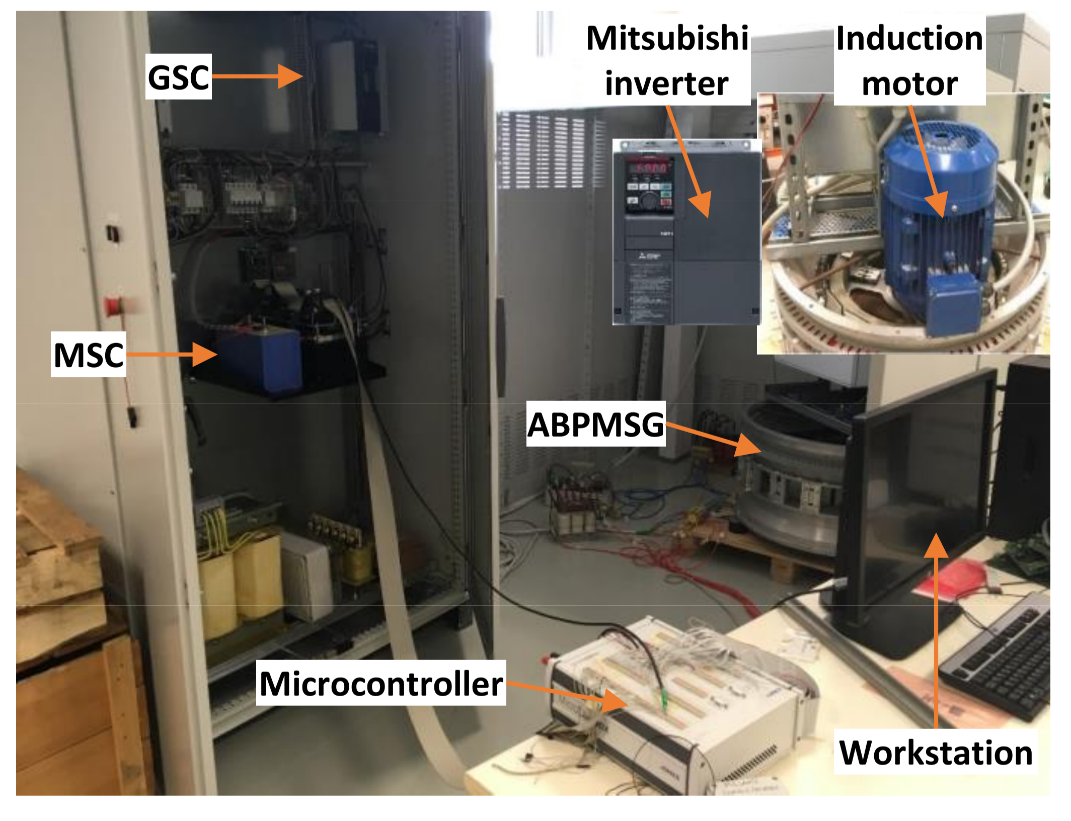
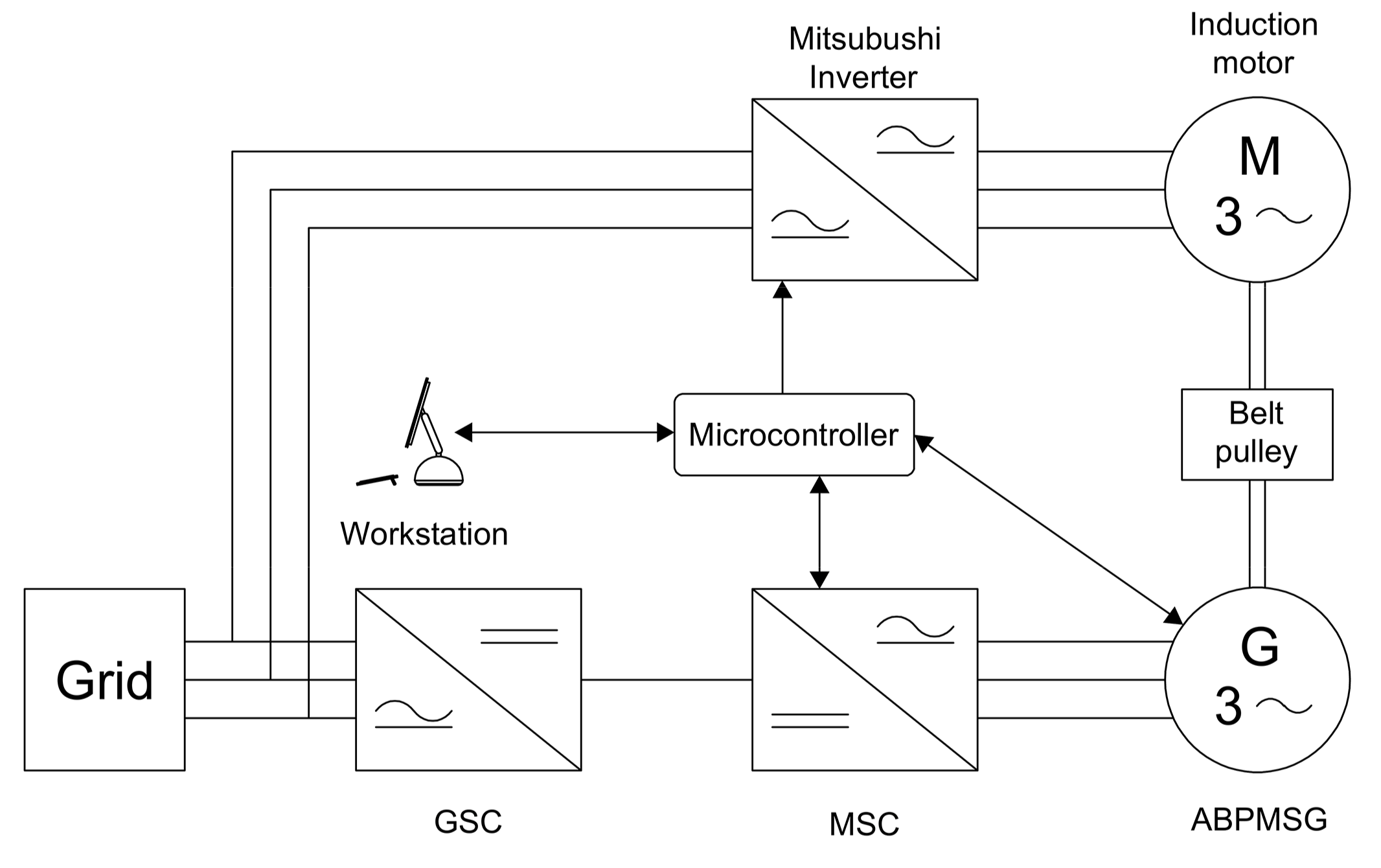
4.1. Test Rig Overview
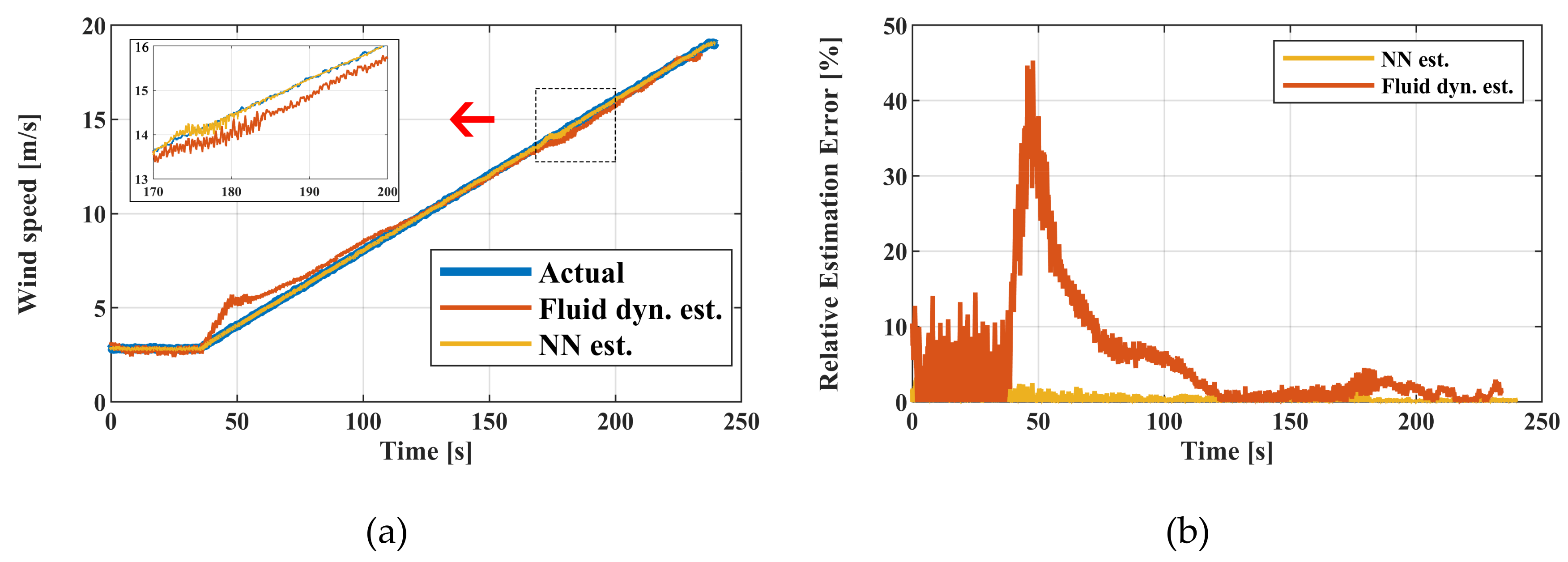
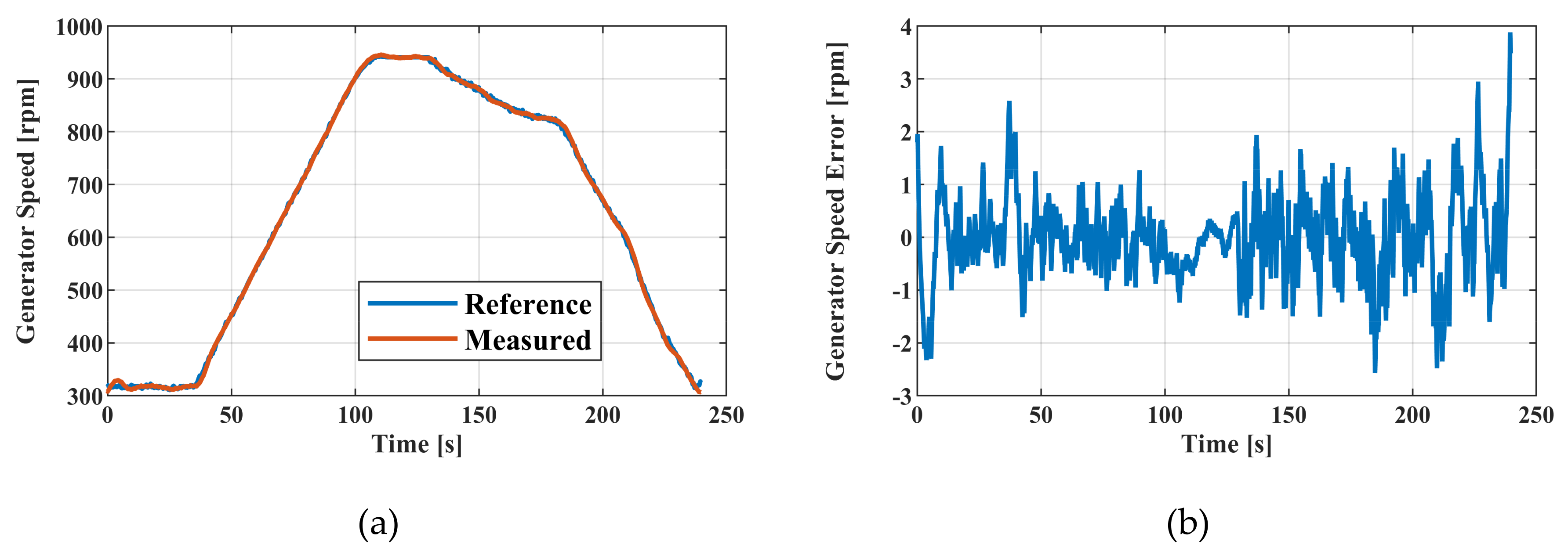
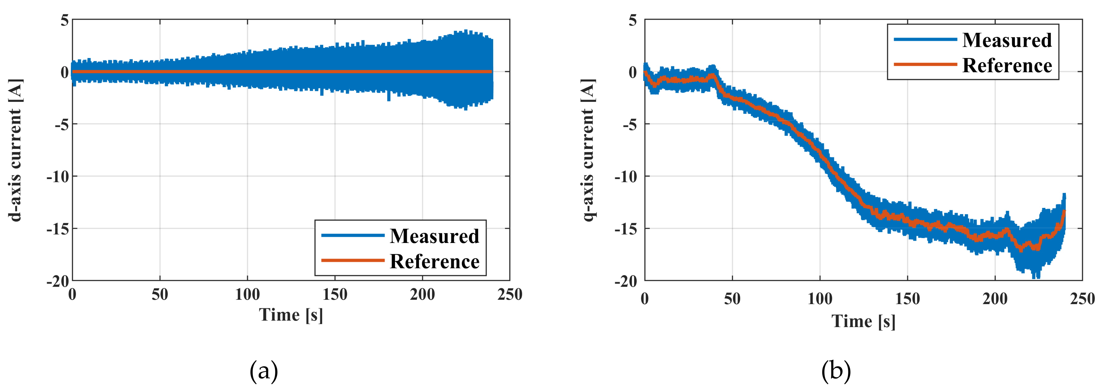
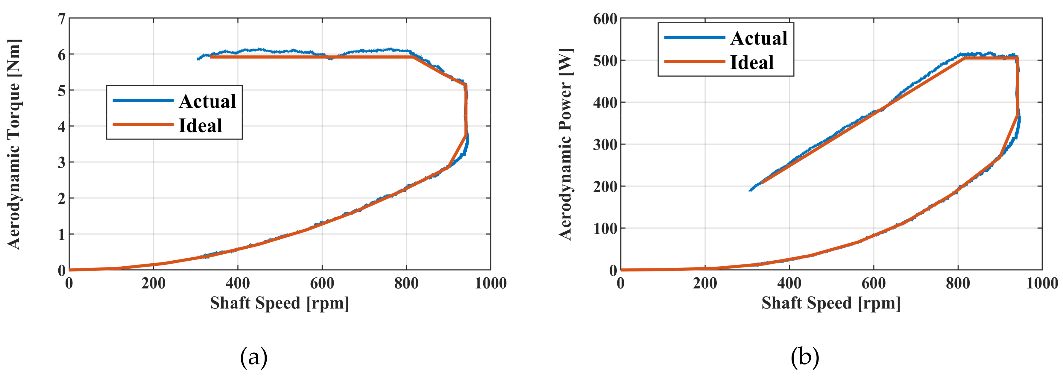
The test rig used for the experimental tests is shown in Figure 10. A dSPACE MicroLabBox d1202 microcontroller was used to execute the test. The DHAWT emulation was achieved by connecting a commercial induction motor (IM) Leporis MS 132S3-2 (which emulates the aerodynamic torque) to a customised edition of the described ABPMSG, reproduced on a reduced scale. The two electric machines were connected through pulleys and belts. The mechanical losses of this transmission have been considered to emulate the behaviour of a direct connection. As suggested in [50,51], the mechanical losses were derived by means of the mechanical power difference between the IM and ABPMSG. The IM is driven in torque control mode by a dedicated Mitsubishi FR A800E inverter. Its torque reference is calculated in real time by adding a mechanical loss torque term to the aerodynamic torque provided by an LUT based on the data of the DHAWT and on (5). The input of this LUT was the actual wind speed and the up-scaled measured shaft speed. Since the ABPSMG used during the test has rated speed and torque smaller than those of the examined DHAWT, a scaling process was performed. This process acts on the four control laws described in Section 3.1, which are used for computing the shaft speed reference and the LUT used for the computation of the torque reference of the IM. The shaft speed references provided by the four control laws were multiplied by the ratio between the rated speed of the reduced-scale ABPMSG and of the DHAWT. Moreover, the maximum torque and rated power values used for the CPC and CTC were downscaled with the same logic. Concerning the IM LUT, the shaft speed input is the measured speed of the ABPMSG multiplied by the inverse of the ratio used for downscaling. Finally, the output of this LUT (aerodynamic torque of the examined DHAWT) was downscaled. The generator side converter is a custom converter composed of three Semikron SEMiX303GB12E4s modules, each containing two IGBT diodes. The main board of this converter also includes current sensors. The grid-side converter is instead a TDE MACNO OPDE AFE ENERGY S 15, in a custom edition for this rig, and it is set to keep 650 V on the DC-link. Table 5 summarises the main parameters of the experimental setup, and Figure 11 shows a logical scheme with the interconnections between the components of the test rig. The control scheme described in Section 3 was carried out in a MATLAB-Simulink environment and then uploaded into the microcontroller.
Fore more information see Supplementary Materials.

4.2. Results

In this section, we discuss the experimental results obtained on the test rig. The shaft speed and the aerodynamic torque and power obtained during the tests were scaled up (multiplied by the ratio between the rated values of the DHAWT and ABPMSG) to compare the results with the ideal regulation curves illustrated in Figure 6 and Figure 7a,b.
In Figure 12a, the actual test wind speed pattern and the wind speed estimated with the model-based and NN WSEs are shown. Figure 12b shows the estimation errors. The actual wind speed pattern was built with a uniformly random noise signal overlapped on a 0.08 slope ramp. An extended operative range was considered, from 2.8 to 18.9 m/s even if the cut-in speed defined above was 2 m/s. The test was accomplished starting from 2.8 m/s to overcome hardware limitations. After a brief initial interval (approximately 35 s), the wind speed ramp started growing until the cut-out speed is reached. Therefore, the test lasted approximately 250 s. The comparison between the WSEs clearly prove the superiority of the proposed NN WSE.
The comparison between the actual and estimated aerodynamic torque is shown in Figure 13a, whereas in Figure 13b, the relative estimation errors are reported. The observers have very similar dynamics and performances: the maximum error is obtained when the wind speed starts increasing, but when the MPPT subregion is finished, T a ^ becomes very reliable until the cut-out speed is reached. Moreover, the adaptive observer exhibits better performance than the LO at low torque values, while at high torque values, the situation is reversed. Among the causes of the estimation error that affects both observers, there are uncertainties in the model parameters ( K c and J ), inaccuracies in the estimation and compensation of the mechanical losses, and inaccuracies of the torque control of the IM. However, this error is acceptable in practise and affects only slightly the performance of the proposed control scheme, as will be shown in the following figures. In conclusion, these results show that the LO can be effectively employed for the estimation of the aerodynamic torque of WECSs as a valid alternative to the adaptive observer proposed in [17].
The comparison between Figure 12 and Figure 13 shows that the estimation of the wind speed with the model-based approach is strongly dependent on the accuracy of the aerodynamic torque estimation. This is particularly evident in the time range between 40 and 60 s. Moreover, Figure 13a shows how the actual aerodynamic torque is characterised by an almost constant trend between 180 s and the end of the test. In this time lapse, the wind speed has overcome 14.5 m/s and the CTC achieves a net of small fluctuations.
Figure 14a shows how the measured ABPMSG rotor speed tracks its reference trajectory very well. The test started with a value of the shaft speed of about 300 rpm; that is the MPPT control reference speed for 2.8 m/s wind speed value. The speed tracking error has also been reported in Figure 14b: the tracking error was restricted to a ±3 rpm range with an average value equal to −0.03 rpm. At the time instant = 110 s, the rated rotor speed was reached, and the control provided a constant rotor speed until the time instant = 130 s, when the rated power was reached. Thus, CSC was achieved.
Figure 15a,b shows the references and measured d-axis and q-axis currents. It can be seen that the measured currents track the references with some oscillations.
To better illustrate the effectiveness of the proposed method, in Figure 16 and Figure 17, the ideal regulation characteristics were compared with the actual scaled ones, depending on rotor speed and wind speed. The actual curves match the ideal ones with a good fit in all wind subregions; therefore, these figures clearly show that the proposed control scheme is effective in all the DHAWT operating ranges. We note that the ideal power curve depicted in Figure 17 (i.e., the same as in Figure 5) cannot be physically exceeded only in the MPPT subregion. In fact, the purpose of the MPPT is to extract the maximum wind power according to the wind turbine conversion efficiency. Thus, in this wind speed subregion, the ideal power curve represents the maximum aerodynamic power that can be physically extracted by the wind turbine. However, in this subregion, the actual aerodynamic power follows the ideal one very precisely. For wind speeds above this subregion, the ideal power curve represents the maximum power that can be extracted without exceeding the safety mechanical limits. In this case, in the CPC and CTC subregions, the actual power slightly exceeds the ideal one because of the control scheme performance. This is mainly caused by the aerodynamic torque estimation error. In fact, as shown in Figure 13b, when the CPC and CTC are performed (after 130 s), the aerodynamic torque estimated by the LO is lower than the actual one. Considering now (14) and (15) because the shaft speed reference is inversely proportional to T a ^ , its value is higher than that achieved without estimation errors. Therefore, the increased shaft speed reference leads the DHAWT to develop an aerodynamic power higher than the ideal one. However, in practise, small deviations are acceptable.
To the best of the authors’ knowledge, the proposed aerodynamic power regulation considering the mechanical constraints of the WECS with a back-to-back power converter topology has not been achieved before in the literature. In fact, even if the CSC and CPC have been performed in [14,20], neither have faced the issue of limiting the aerodynamic torque. Moreover, in [14], a WECS with a passive three-phase diode rectifier and a boost converter is considered. The control scheme is largely dependent on this power converter topology, and is not suitable for the application on the WECS considered in the present work. In fact, the control laws proposed in [14] explicitly refer to the generator rectification voltage (regulated by the boost converter) to achieve the ideal power characteristic, while in the present work, this voltage is held constant by the GSC. For a thorough evaluation of the performance achieved with the proposed control scheme, it is possible and useful to compare the results achieved in [20]. In this study, the generator speed was regulated with a PID speed controller whose output was the reference current of a buck converter connected to a battery bank; therefore, the FOC was not performed. Moreover, the control scheme avoids the need for wind speed measurement or estimation and makes use of an aerodynamic power observer and shaft speed measurement. Specifically, in [20], the MPPT was performed with the power signal feedback (PSF) method, while the CPC was performed with a closed loop with another PID regulator. Table 6 summarises the main features of the compared control schemes. Figure 9 and Figure 10 shown in [20] can be compared to Figure 16b and Figure 17, respectively. It can be seen how the control schemes achieved overall similar performances until the CPC. This comparison definitively clarifies the originality and effectiveness of the proposed WECS. Finally, we want to highlight that the merit of the performance achieved with the control scheme proposed in this paper has to be also attributed to the accurate wind speed estimation achieved with the designed NN. In fact, an accurate wind speed estimation is crucial for optimal shaft speed reference computation in the MPPT and CTC regions. Moreover, an accurate wind speed estimation allows for a timely and proper transition between the four designed control laws.

5. Conclusions

In this paper, an innovative variable structure control scheme for a small-scale VSFP DHAWT over the entire wind speed range is proposed. This control strategy was implemented considering an ABMPSG grid-connected through a back-to-back connection of two PWM three-phase inverters. An ideal power regulation characteristic depending on wind speed has been considered to maximise the power extraction, while ensuring the respect of the safety mechanical limits of the WECS. A VSC was designed to achieve the ideal regulation characteristic. This controller regulates the shaft speed of the DHAWT according to four control laws performed in four wind speed subregions. In the low-speed region, MPPT was performed with the optimal TSR method. Instead, the high wind speed region has been divided into three subregions, CSC, CPC, and CTC, which are used to avoid exceeding the rated shaft speed, the rated aerodynamic power, and the maximum aerodynamic torque of the DHAWT. Moreover, an LO has been proposed for the estimation of the aerodynamic torque necessary for CPC and CTC implementation. Finally, a shallow NN was designed for the estimation of the wind speed necessary for the transition between the control laws and the MPPT control and CTC implementation. The proposed control scheme was validated through tests executed on a laboratory setup. These tests were performed considering a ramp wind speed pattern to explore the entire operating range of the DHAWT. The results showed that the overall control strategy was successful in tracking the ideal power regulation characteristic. Moreover, to better evaluate the performances achieved with the proposed control scheme, comparisons with other solutions from the literature have been made. The LO achieved very similar performances to those of an adaptive ATO, and this demonstrates its effectiveness in the estimation of the aerodynamic torque. The NN WSE showed high performance and is clearly more accurate than a model-based WSE whose performances are influenced by the estimation errors on the aerodynamic torque. Finally, a comparison with a previously reported control scheme further demonstrates the effectiveness and originality of the proposed scheme.

Supplementary Materials

The following are available online at https://doi.org/10.5281/zenodo.3910928.

Author Contributions

Conceptualisation, E.B., G.L.C. and F.C.; methodology, D.C., G.T., E.B. and F.C.; software, D.C. and G.T.; validation, G.L.C. and V.G.M.; formal analysis, D.C.; investigation, D.C., G.T., E.B. and V.G.M.; resources, V.G.M. and F.C.; data curation, F.C.; writing—Original draft preparation, D.C., G.T. and E.B.; writing—Review and editing, G.L.C., V.G.M. and F.C.; visualisation, D.C., G.T. and E.B.; supervision, G.L.C. and F.C.; project administration, V.G.M. and F.C.; funding acquisition, F.C. All authors have read and agreed to the published version of the manuscript.

Funding

This work was partially supported by the project “Wind Micro-Turbine Networks for Urban Areas” (in Italian “Reti di microturbine eoliche per la produzione diffusa di energia in ambito urbano”)—Fondazione Puglia, Italy.

Acknowledgments

The authors would like to thank Rinaldo Consoletti for his technical support concerning the experimental tests.

Conflicts of Interest

The authors declare no conflict of interest.

Appendix A

Considering the parameter uncertainties relative to J and K c , (21) can be rewritten as
B ^ = B + · B
From this expression of B ^ results, the differential error expressed by (23) can now be expressed as
e ˙ = A e L C e   + · B u = A L C e + · B u
Thus, the error will have a term asymptotically convergent to zero ( e 1 t ) and another ( e 2 u ) that is a function of u :
e = e 1 t + e 2 u
From (17), u = i s q and (A3) can be rewritten as
e = e 1 t + e 2 i s q
Moreover, neglecting the dynamic of the error of the LO, we can assume this approximate equation:
T a ^ = J d ω m d t + K c i s q +   e 2 i s q
This approximate equation is based on the model of the system observed by the LO, and on the error due to parameter uncertainties. Now, we demonstrate that under the previous assumptions, v cannot be expressed as a univocal function of T a ^ and ω m .
Theorem 1.
There is no function f v such that   v = f v T a ^ , ω m .
Proof of Theorem 1.
To prove this theorem, it should be demonstrated that two different operating conditions of the wind turbine at different wind speed values, equal shaft speed, and estimated aerodynamic torque values can exist.
Let us assume that during the test of the WECS with the anemometer, the two following values of the measured wind and shaft speed, q-axis current, and estimated aerodynamic torque are registered in two different time instants t 1 and t 2 :
ω m 1 , v 1 , i s q 1 , T a 1 ^ ω m 2 , v 2 , i s q 2 , T a 2 ^
Moreover, let us assume that:
ω m 1 = ω m 2 = ω m 12 v 1 v 2 i s q 1 i s q 2
In this case, as can be seen from Figure 7b, the actual aerodynamic torque values in these two time instants are different:
T a 1 ω m 12 , v 1 T a 2 ω m 12 , v 2
However, because of the presence of estimation error, the following can be verified:
T a 1 ^ = T a 2 ^ = T a 12 ^
In fact, in these two time instants (10) is satisfied:
J   d ω m d t t 1 = T a 1 K c i s q 1 T a v ω m 12
J   d ω m d t t 2 = T a 2 K c i s q 2 T a v ω m 12
and from (A5), (A9) and (A10) results:
T a 1 ^ = J   d ω m d t t 1 + K c i s q 1 +   e 2 i s q 1 = T a 1 T a v ω m 12 + e 2 i s q 1  
T a 2 ^ = J   d ω m d t t 2 + K c i s q 2 +   e 2 i s q 2 = T a 2 T a v ω m 12 + e 2 i s q 2
Thus, T a 1 ^ = T a 2 ^ if and only if
T a 1 + e 2 i s q 1 = T a 2 + e 2 i s q 2
In general, can exist for values of T a 1 ,   T a 2 , i s q 1 and i s q 2 that satisfy this condition. Thus, the theorem has been demonstrated. □
At this point, it will be demonstrated that the wind speed can be expressed as a univocal function of T a ^ ω m and i s q .
Theorem 2.
There exists a function f v such that   v = f v T a ^ , ω m , i s q .
Proof of Theorem 2.
To prove this theorem, it should be demonstrated that two different operating conditions of the wind turbine at different wind speed values and equal shaft speed, the estimated aerodynamic torque and q-axis current values cannot exist.
Let us consider two vectors, as in (A6) and assume that:
ω m 1 = ω m 2 = ω m 12 v 1 v 2 i s q 1 = i s q 2 = i s q 12
By repeating the previous procedure, it can be stated that T a 1 ^ = T a 2 ^ is verified if and only if
T a 1 + e 2 i s q 12 = T a 2 + e 2 i s q 12 T a 1 = T a 2
However, T a 1 T a 2 from (A7). Thus, two different operating conditions of the wind turbine at different wind speed values and equal shaft speed, estimated aerodynamic torque, and q-axis current values cannot exist. Therefore, there exists a function f v such that v = f v T a ^ , ω m , i s q . □

Appendix B

The LO designed in Section 3 was converted in the discrete-time domain for the experimental tests. In this time domain, the state of an LTI system is expressed by
x k + 1 = A d x k + B d u k y k = C d x k
where time dependence for each variable is highlighted: e.g., k indicates the k t h sample. The discrete LO likewise is described by the following equations:
x ^ k + 1 = A d ^   x ^ k + B d ^   u k + L d   y k y ^ k = C d   x ^ k
where:
A d ^ = 0 T s J 0 0 ,   B d ^ = T s K c J 0 ,   C d = 1 0
The estimation error is
e k + 1 = A d L d C d   e k
In the discrete-time domain, the matrix L d was designed to place the eigenvalues of the matrix A d L d C d inside the unit radius circle. The transition between the continuous and discrete-time domains does not affect the property of observability.

References

  1. Lumbreras, C.; Guerrero, J.M.; Fernandez, D.; Reigosa, D.D.; González-Moral, C.; Briz, F. Analysis and Control of the Inductorless Boost Rectifier for Small-Power Wind-Energy Converters. IEEE Trans. Ind. Appl. 2018, 55, 689–700. [Google Scholar] [CrossRef]
  2. Micallef, D.; van Bussel, G. A Review of Urban Wind Energy Research: Aerodynamics and Other Challenges. Energies 2018, 11, 2204. [Google Scholar] [CrossRef] [Green Version]
  3. Rodriguez-Hernandez, O.; Martinez, M.; Lopez-Villalobos, C.; Garcia, H.; Campos-Amezcua, R. Techno-Economic Feasibility Study of Small Wind Turbines in the Valley of Mexico Metropolitan Area. Energies 2019, 12, 890. [Google Scholar] [CrossRef] [Green Version]
  4. Gough, M.; Lotfi, M.; Castro, R.; Madhlopa, A.; Khan, A.; Catalão, J.P. Urban Wind Resource Assessment: A Case Study on Cape Town. Energies 2019, 12, 1479. [Google Scholar] [CrossRef] [Green Version]
  5. Elnaggar, M.; Edwan, E.; Ritter, M. Wind energy potential of Gaza using small wind turbines: A feasibility study. Energies 2017, 10, 1229. [Google Scholar] [CrossRef]
  6. Acosta, J.L.; Combe, K.; Djokic, S.Ž.; Hernando-Gil, I. Performance assessment of micro and small-scale wind turbines in urban areas. IEEE Syst. J. 2011, 6, 152–163. [Google Scholar] [CrossRef]
  7. Szabó, L. A survey on modular variable reluctance generators for small wind turbines. IEEE Trans. Ind. Appl. 2019, 55, 2548–2557. [Google Scholar] [CrossRef]
  8. Palmieri, M.; Bozzella, S.; Cascella, G.L.; Bronzini, M.; Torresi, M.; Cupertino, F. Wind Micro-Turbine Networks for Urban Areas: Optimal Design and Power Scalability of Permanent Magnet Generators. Energies 2018, 11, 2759. [Google Scholar] [CrossRef] [Green Version]
  9. Shafiei, A.; Dehkordi, B.M.; Farhangi, S.; Kiyoumarsi, A. Overall power control strategy for small-scale WECS incorporating flux weakening operation. IET Renew. Power Gener. 2016, 10, 1264–1277. [Google Scholar] [CrossRef]
  10. Maher, R.A.; Abdelsalam, A.K.; Dessouky, Y.G.; Nouman, A. High performance state-flow based MPPT technique for micro WECS. IET Renew. Power Gener. 2019, 13, 3009–3021. [Google Scholar] [CrossRef]
  11. Lumbreras, C.; Guerrero, J.M.; Garcia, P.; Briz, F.; Reigosa, D.D. Control of a small wind turbine in the high wind speed region. IEEE Trans. Power Electron. 2015, 31, 6980–6991. [Google Scholar] [CrossRef]
  12. Shafiei, A.; Dehkordi, B.M.; Kiyoumarsi, A.; Farhangi, S. A control approach for a small-scale PMSG-based WECS in the whole wind speed range. IEEE Trans. Power Electron. 2017, 32, 9117–9130. [Google Scholar] [CrossRef]
  13. Lee, J.; Kim, Y.S. Sensorless fuzzy-logic-based maximum power point tracking control for a small-scale wind power generation system with a switched-mode rectifier. IET Renew. Power Gener. 2016, 10, 194–202. [Google Scholar] [CrossRef]
  14. Chen, J.; Chen, J.; Gong, C. New overall power control strategy for variable-speed fixed-pitch wind turbines within the whole wind velocity range. IEEE Trans. Ind. Electron. 2012, 60, 2652–2660. [Google Scholar] [CrossRef]
  15. Dalala, Z.M.; Zahid, Z.U.; Lai, J.S.J. New overall control strategy for small-scale WECS in MPPT and stall regions with mode transfer control. IEEE Trans. Energy Conv. 2013, 28, 1082–1092. [Google Scholar] [CrossRef]
  16. Hui, J.C.; Bakhshai, A.; Jain, P.K. An energy management scheme with power limit capability and an adaptive maximum power point tracking for small standalone PMSG wind energy systems. IEEE Trans. Power Electron. 2015, 31, 4861–4875. [Google Scholar] [CrossRef]
  17. Guerrero, J.M.; Lumbreras, C.; Reigosa, D.D.; Garcia, P.; Briz, F. Control and emulation of small wind turbines using torque estimators. IEEE Trans. Ind. Appl. 2017, 53, 4863–4876. [Google Scholar] [CrossRef] [Green Version]
  18. Chen, J.; Lin, T.; Wen, C.; Song, Y. Design of a unified power controller for variable-speed fixed-pitch wind energy conversion system. IEEE Trans. Ind. Electron. 2016, 63, 4899–4908. [Google Scholar] [CrossRef]
  19. Senanayaka, J.S.L.; Karimi, H.R.; Robbersmyr, K.G. A novel soft-stall power control for a small wind turbine. In Proceedings of the IEEE 26th International Symposium on Industrial Electronics (ISIE), Edinburgh, Scotland, UK, 19 June 2017; pp. 940–945. [Google Scholar]
  20. Jiawei, C.; Changyun, W.; Yongduan, S. Power control strategy for variable-speed fixed-pitch wind turbines. In Proceedings of the 13th International Conference on Control Automation Robotics & Vision (ICARCV), Singapore, 10 December 2014; pp. 559–564. [Google Scholar]
  21. Morimoto, S.; Nakayama, H.; Sanada, M.; Takeda, Y. Sensorless output maximization control for variable-speed wind generation system using IPMSG. IEEE Trans. Ind. Appl. 2005, 41, 60–67. [Google Scholar] [CrossRef]
  22. Wang, Y.F.; Yang, L.; Wang, C.S.; Li, W.; Qie, W.; Tu, S.J. High step-up 3-phase rectifier with fly-back cells and switched capacitors for small-scaled wind generation systems. Energies 2015, 8, 2742–2768. [Google Scholar] [CrossRef]
  23. Do, T.D. Disturbance observer-based fuzzy SMC of WECSs without wind speed measurement. IEEE Access 2016, 5, 147–155. [Google Scholar] [CrossRef]
  24. Corradini, M.L.; Ippoliti, G.; Orlando, G. Robust control of variable-speed wind turbines based on an aerodynamic torque observer. IEEE Trans. Control Syst. Technol. 2013, 21, 1199–1206. [Google Scholar] [CrossRef]
  25. Merabet, A. Adaptive sliding mode speed control for wind energy experimental system. Energies 2018, 11, 2238. [Google Scholar] [CrossRef]
  26. Nouali, S.; Ouali, A. Multi-layer neural network for sensorless MPPT control for wind energy conversion system using doubly fed twin stator induction generator. In Proceedings of the Eighth International Multi-Conference on Systems, Signals & Devices, Sousse, Tunisia, 22 March 2011; pp. 1–7. [Google Scholar]
  27. Martyanov, A.; Martyanov, N.; Sirotkin, E. State Observer for Variable Speed Wind Turbine. In Proceedings of the International Ural Conference on Green Energy (UralCon), Chelyabinsk, Russia, 4 October 2018; pp. 97–100. [Google Scholar]
  28. Liu, H.; Locment, F.; Sechilariu, M. Integrated Control for Small Power Wind Generator. Energies 2018, 11, 1217. [Google Scholar] [CrossRef] [Green Version]
  29. Qiao, W.; Yang, X.; Gong, X. Wind speed and rotor position sensorless control for direct-drive PMG wind turbines. IEEE Trans. Ind. Appl. 2011, 48, 3–11. [Google Scholar] [CrossRef]
  30. Liu, H.; Locment, F.; Sechilariu, M. Experimental analysis of impact of maximum power point tracking methods on energy efficiency for small-scale wind energy conversion system. IET Renew. Power Gener. 2016, 11, 389–397. [Google Scholar] [CrossRef]
  31. Saleh, S.A. Testing the performance of a resolution-level MPPT controller for PMG-based wind energy conversion systems. IEEE Trans. Ind. Appl. 2017, 53, 2526–2540. [Google Scholar] [CrossRef]
  32. Hussain, J.; Mishra, M.K. An Efficient Wind Speed Computation Method Using Sliding Mode Observers in Wind Energy Conversion System Control Applications. IEEE Trans. Ind. Appl. 2019, 56, 730–739. [Google Scholar] [CrossRef]
  33. Yaylacı, E.K. Discrete-time integral terminal sliding mode based maximum power point controller for the PMSG-based wind energy system. IET Power Electron. 2019, 12, 3688–3696. [Google Scholar]
  34. Yazici, İ.; Yaylaci, E.K. Maximum power point tracking for the permanent magnet synchronous generator-based WECS by using the discrete-time integral sliding mode controller with a chattering-free reaching law. IET Power Electron. 2017, 10, 1751–1758. [Google Scholar] [CrossRef]
  35. Wei, C.; Zhang, Z.; Qiao, W.; Qu, L. An adaptive network-based reinforcement learning method for MPPT control of PMSG wind energy conversion systems. IEEE Trans. Power Electron. 2016, 31, 7837–7848. [Google Scholar] [CrossRef]
  36. Werle, M.; Presz, W. Ducted Wind/Water Turbines and Propellers Revisited. J. Propul. Power 2008, 24, 1146–1150. [Google Scholar] [CrossRef]
  37. Torresi, M.; Postiglione, N.; Filianoti, P.F.; Fortunato, B.; Camporeale, S.M. Design of a ducted wind turbine for offshore floating platforms. Wind Eng. 2016, 40, 468–474. [Google Scholar] [CrossRef]
  38. Khamlaj, T.A.; Rumpfkeil, M.P. Analysis and optimization of ducted wind turbines. Energy 2018, 162, 1234–1252. [Google Scholar] [CrossRef]
  39. Grant, A.; Johnstone, C.; Kelly, N. Urban wind energy conversion: The potential of ducted turbines. Renew. Energy 2008, 33, 1157–1163. [Google Scholar] [CrossRef] [Green Version]
  40. Ali, M.A.S.; Mehmood, K.K.; Baloch, S.; Kim, C.H. Wind-Speed Estimation and Sensorless Control for SPMSG-Based WECS Using LMI-Based SMC. IEEE Access 2020, 8, 26524–26535. [Google Scholar] [CrossRef]
  41. Zhao, H.; Wu, Q.; Rasmussen, C.N.; Blanke, M. L1 Adaptive Speed Control of a Small Wind Energy Conversion System for Maximum Power Point Tracking. IEEE Trans. Energy Convers. 2014, 29, 576–584. [Google Scholar] [CrossRef] [Green Version]
  42. Orlando, N.A.; Liserre, M.; Monopoli, V.G.; Dell’Aquila, A. Speed sensorless control of a PMSG for small wind turbine systems. In Proceedings of the IEEE International Symposium on Industrial Electronics, Seoul, Korea, 5–8 July 2009; pp. 1540–1545. [Google Scholar]
  43. Zhang, Z.; Zhao, Y.; Qiao, W.; Qu, L. A space-vector-modulated sensorless direct-torque control for direct-drive PMSG wind turbines. IEEE Trans. Ind. Appl. 2014, 50, 2331–2341. [Google Scholar] [CrossRef]
  44. Li, D.Y.; Cai, W.C.; Li, P.; Jia, Z.J.; Chen, H.J.; Song, Y.D. Neuroadaptive variable speed control of wind turbine with wind speed estimation. IEEE Trans. Ind. Electron. 2016, 63, 7754–7764. [Google Scholar] [CrossRef]
  45. Hui, J.C.; Bakhshai, A.; Jain, P.K. A sensorless adaptive maximum power point extraction method with voltage feedback control for small wind turbines in off-grid applications. IEEE Trans. Emerg. Sel. Top. Power Electron. 2015, 3, 817–828. [Google Scholar] [CrossRef]
  46. Syahputra, R.; Soesanti, I. Performance Improvement for Small-Scale Wind Turbine System Based on Maximum Power Point Tracking Control. Energies 2019, 12, 3938. [Google Scholar] [CrossRef] [Green Version]
  47. Uddin, M.N.; Patel, N. Maximum power point tracking control of IPMSG incorporating loss minimization and speed sensorless schemes for wind energy system. IEEE Trans. Ind. Electron. 2015, 52, 1902–1912. [Google Scholar] [CrossRef]
  48. Qian, X.; Huang, H.; Chen, X.; Huang, T. Generalized Hybrid Constructive Learning Algorithm for Multioutput RBF Networks. IEEE Trans. Cybern. 2017, 47, 3634–3648. [Google Scholar] [CrossRef] [PubMed]
  49. Wilamowski, B.M.; Yu, H. Improved Computation for Levenberg–Marquardt Training. IEEE Trans. Neural Netw. 2010, 21, 930–937. [Google Scholar] [CrossRef] [PubMed]
  50. Dereyne, S.; Defreyne, P.; Algoet, E.; Derammelaere, S.; Stockman, K. An efficiency measurement campaign on belt drives. Proceedings of 9th International Conference on Energy Efficiency in Motor Driven Systems, Helsinky, Finland, 15–17 September 2015. [Google Scholar]
  51. Chen, T.F.; Lee, D.W.; Sung, C.K. An experimental study on transmission efficiency of a rubber V-belt CVT. Mech. Mach. Theory 1998, 33, 351–363. [Google Scholar] [CrossRef]
Figure 1. Wind energy conversion system (WECS) schematic.
Energies 13 04647 g001
Figure 2. Rendering of the DHAWT–ABPMSG system.
Energies 13 04647 g002
Figure 3. DHAWT characteristic curve.
Energies 13 04647 g003
Figure 4. Variable structure controller.
Energies 13 04647 g004
Figure 5. Subregions of the DHAWT operating range.
Energies 13 04647 g005
Figure 6. Look-up tables (LUT)s of the control algorithm. (a) Shaft speed reference during MPPT control. (b) Tip-speed ratio (TSR), during constant torque control (CTC).
Energies 13 04647 g006
Figure 7. Regulation characteristics. (a) Regulation curve in ω m P a plane. (b) Regulation curve in ω m T a plane.
Energies 13 04647 g007
Figure 8. Shallow NN with twenty hidden layers.
Energies 13 04647 g008
Figure 9. C p λ 3 λ characteristic.
Energies 13 04647 g009
Figure 10. Experimental test rig.
Energies 13 04647 g010
Figure 11. The test rig’s logical scheme.
Energies 13 04647 g011
Figure 12. Wind speed: (a) actual and estimated wind speed pattern; (b) relative (percentage) estimation errors.
Energies 13 04647 g012
Figure 13. Aerodynamic torque: (a) actual and estimated aerodynamic torque; (b) relative (percentage) estimation errors.
Energies 13 04647 g013
Figure 14. ABPMSG rotor speed: (a) speed reference and measured rotor speed; (b) absolute speed tracking error.
Energies 13 04647 g014
Figure 15. Comparison between reference and measured currents: (a) d-axis current; (b) q-axis current.
Energies 13 04647 g015
Figure 16. Regulation characteristics comparisons: (a) ideal and actual aerodynamic torque depending on shaft speed; (b) ideal and actual aerodynamic power depending on shaft speed.
Energies 13 04647 g016
Figure 17. Actual and ideal aerodynamic power curves depending on wind speed.
Energies 13 04647 g017
Table 1. Ducted wind turbine parameters.
SymbolQuantityValue
P r a t e d Rated Power 0.5   kW
ω r a t e d Rated Speed 941   rpm
T m a x Maximum Torque 59   Nm
R Blade Radius 0.51   m
m b Blade Mass 0.110   Kg
J Total Inertia 1.193   Kgm 2
λ m a x Optimal TSR 6
C p m a x Optimal Power Coefficient1.048
Table 2. ABPMSG parameters.
SymbolQuantityValue
P n Rated Power 0.8   kW
ω n Rated Speed 941   rpm
I n Rated Current 1.55   A
L s Stator Inductance 1.04   · 10 8   H
R s Phase Resistance34.64 Ω
ψ P M PM Flux Linkage 7   · 10 2   W b
n p Number of Pole Pairs50
Table 3. Shaft speed control laws.
Wind Speed RangeControl Law
v c i < v < v s p d ω m * = ω L U T * v
v s p d < v < v r a t e d ω m * = ω r a t e d
v r a t e d < v < v t r q ω m * = P r a t e d T ^ a
v t r q < v < v c o ω m * = T m a x   ω * T ^ a
Table 5. Parameters of the experimental setup.
Parameters Value
ABPMSG
Rated Torque 5.5 Nm
Rated Speed 180 rpm
Rated Current 20   A
Stator Resistance 0.33 Ω
Stator Inductance 0.274   mH
PM Flux Linkage 0.013   W b
Number of pole pairs 15
Total inertia (ABPMSG + IM) 0.148   Kg * m 2
IM
Rated Speed 2930 rpm
Rated Power 9.2 kW
Table 6. Main features of the compared WECS control schemes.
Main FeaturesVSC + LO (Proposed in This Paper)Control Scheme Proposed in [20]
Wind turbineVSFP Ducted HAWTConventional VSFP wind turbine
Electrical generatorABPMSGConventional PMSG
Power converter topologyGrid connected back-to-back PWM invertersPassive diode rectifier + buck converter connected to a battery bank
MPPT control methodOptimal TSRM
odel-based approach with wind speed estimation
PSF
Model-based approach with aerodynamic power estimation
CSC methodFOC with a PI speed closed loopPID speed closed loop (no FOC)
CPC methodOpen loop regulationPID aerodynamic power closed loop
CTC methodOpen loop regulationNot performed
Table 4. Wind speed subregion thresholds.
ThresholdSpeed
v c i 2   m / s
v s p d 9   m / s
v p w r 10.4   m / s
v t r q 14.5   m / s
v c o 18.9   m / s

