Inertial Optimization Based Two-Step Methods for Solving Equilibrium Problems with Applications in Variational Inequality Problems and Growth Control Equilibrium Models

Abstract

This manuscript aims to incorporate an inertial scheme with Popov’s subgradient extragradient method to solve equilibrium problems that involve two different classes of bifunction. The novelty of our paper is that methods can also be used to solve problems in many fields, such as economics, mathematical finance, image reconstruction, transport, elasticity, networking, and optimization. We have established a weak convergence result based on the assumption of the pseudomonotone property and a certain Lipschitz-type cost bifunctional condition. The stepsize, in this case, depends upon on the Lipschitz-type constants and the extrapolation factor. The bifunction is strongly pseudomonotone in the second method, but stepsize does not depend on the strongly pseudomonotone and Lipschitz-type constants. In contrast, the first convergence result, we set up strong convergence with the use of a variable stepsize sequence, which is decreasing and non-summable. As the application, the variational inequality problems that involve pseudomonotone and strongly pseudomonotone operator are considered. Finally, two well-known Nash–Cournot equilibrium models for the numerical experiment are reviewed to examine our convergence results and show the competitive advantage of our suggested methods.

1. Introduction

An Equilibrium problem (EP) was originally started in the unifying feature by Blum and Oettli [1] in 1994 and provided a detailed investigation of their theoretical properties. This study contributes significantly to the advancement of applied and pure science. This problem is primarily related to Ky Fan Inequity due to his early contributions to this field [2]. It has been established that the equilibrium problem theory has set up an unique approach to investigate an immense range of topics that have appeared in social and physical science. For instance, it might involve physical or mechanical structures, chemical processes [3], the distribution of traffic over computer, and telecommunication networks or public roads [4,5,6,7]. In economics, it often refers to production competition [8] or the dynamics of offer and demand [9], exploiting the mathematical model of non-cooperative games and the analogous equilibrium concept by Nash [10,11]. The problem of equilibrium, as a particular case, includes many mathematical problems as a particular case, such as the variational inequality problems (VIP), problems of minimization, the fixed point problems, Nash equilibrium of non-cooperative games, complementarity problems, and saddle point problem (see e.g., [1,12]).

On the other hand, iterative methods are efficient techniques for determining the approximate solution of an equilibrium problem. In that case, two major approaches that are well-known i.e., the proximal point method [13] and auxiliary problem principle [14]. The proximal point method strategy was initially developed by Martinet [15] for the monotone variational inequality problems and later Rockafellar [16] extends this approach for monotone operators. Moudafi [13] proposed the proximal point method for monotone equilibrium problems. Konnov [17] also suggests a different interpretation of the proximal point method with weaker assumptions for equilibrium problems.

In addition, inertial-type methods are additionally significant, depending on the heavy-ball methods of the second-order time dynamic system. Polyak began by considering inertial extrapolation as an acceleration procedure to deal with the problem of smooth convex minimization. Inertial-type algorithms are two-step iterative schemes, and the next iteration is determined by using the previous two iterations and it can be viewed as an accelerating step of the iterative sequence. A large number of methods are the earliest, being set up for solving the problem (EP) in finite and infinite-dimensional spaces, such as the proximal point-like methods [13,18], the extragradient methods [19,20,21,22,23], the subgradient extragradient methods [24,25,26], the inertia methods [27,28,29,30,31,32] and others in [33,34].

In this work, our focus is on the proximal point method, in particular projection methods, which are well established and technically easy to implement due to their convenient numerical computation. This manuscript aims to suggest two modifications of the results that appeared in [21,35,36] by applying the inertial scheme that is useful for speeding up the iteration process. The first result includes the two-step inertial Popov’s extragradient method for determining a numerical solution to the pseudomonotone equilibrium problems and the weak convergence of the suggested method is achieved based on the standard assumptions. We also propose an alternative inertial-type method, the second variant of the first method. The second method does not need any information regarding the Lipschitz-type and strongly pseudomonotone constants of a bifunction. A practical explanation for the second method is that it uses a diminishing and non-summable sequence of non-negative real numbers, which are useful in achieving the strong convergence.

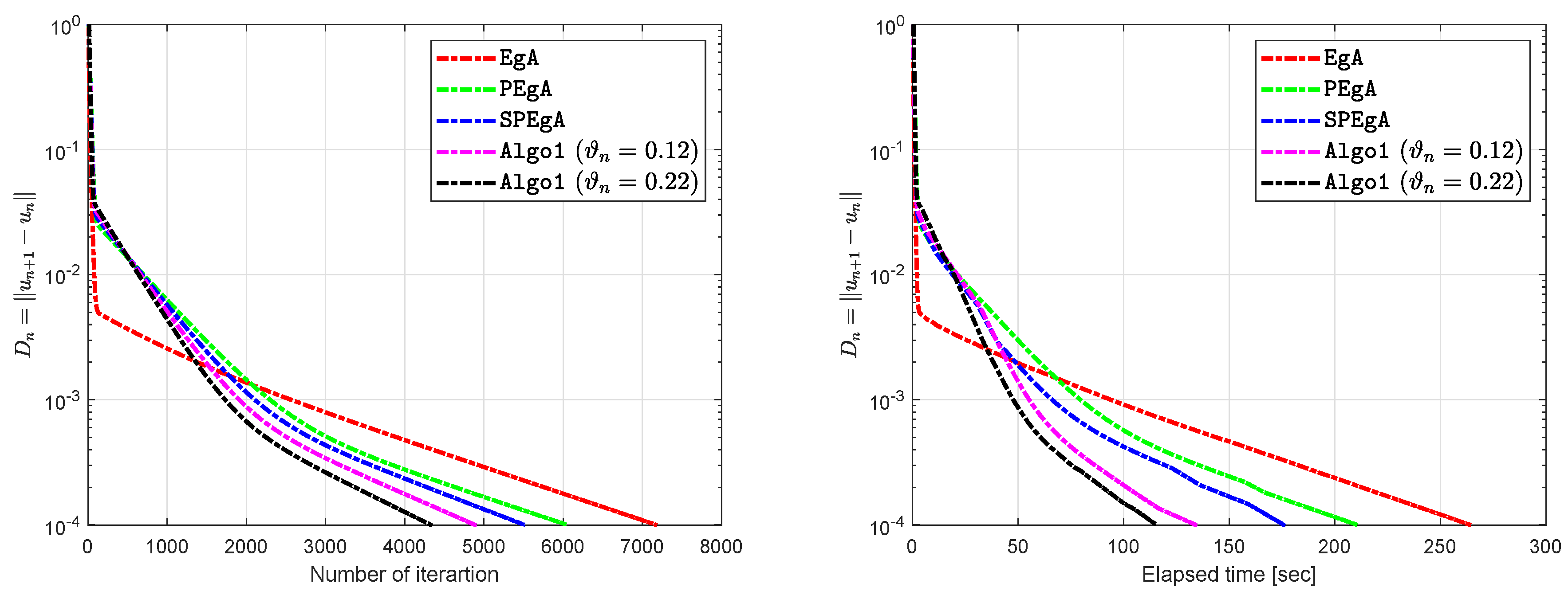
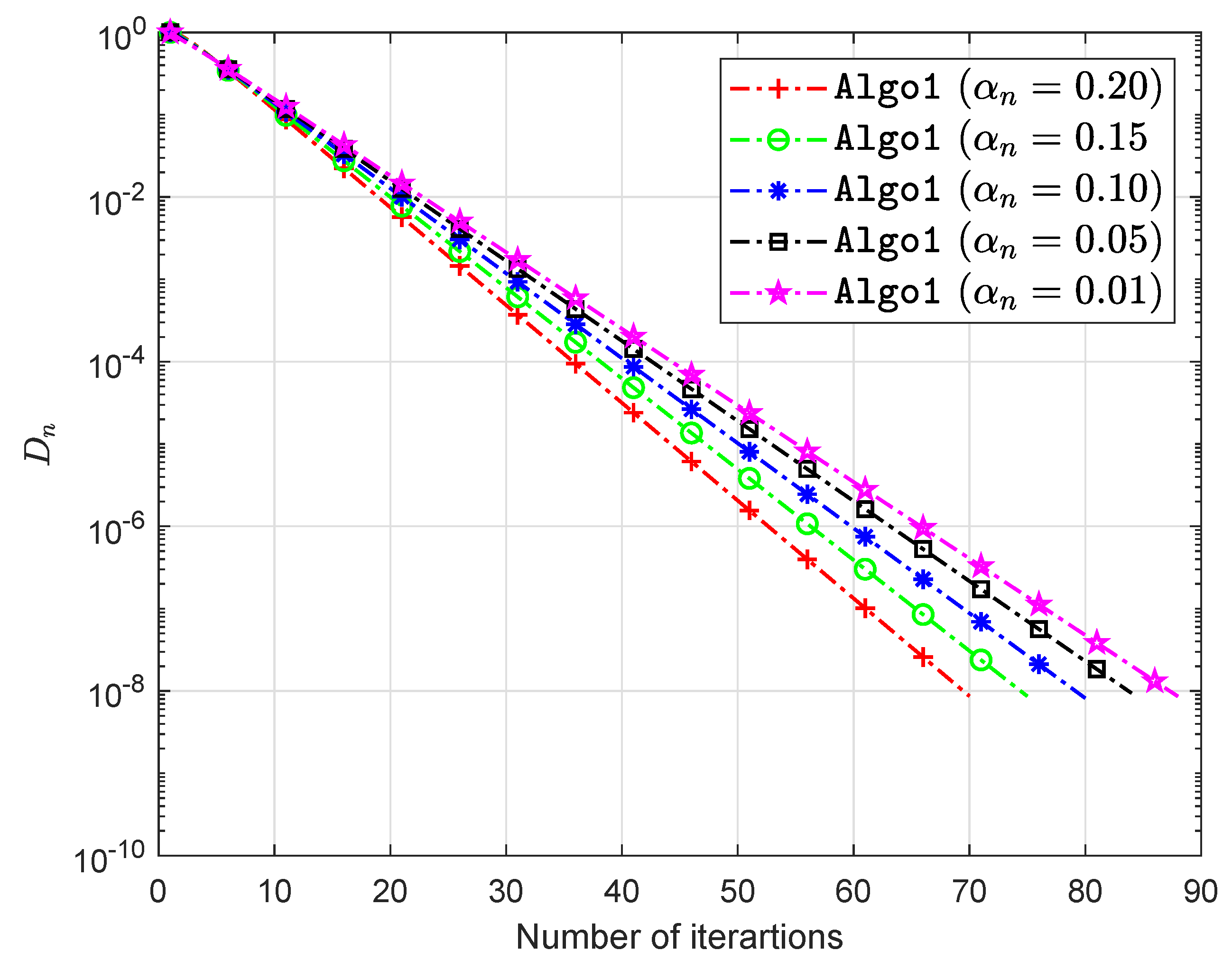
This manuscript is arranged, as follows: in Section 2, we provide some essential definitions and useful results. Section 3 and Section 4 include all of our main methods and corresponding convergence results. Section 5 provides the methods for variational inequality problems. Section 6 sets out the numerical tests to show the numerical efficiency of the proposed methods for the test problems based on the Nash–Cournot equilibrium model compare to other existing methods.

2. Background

Let K be a non-empty, convex, and closed subset of the Hilbert space $\mathbb{E}$. Let $H:K\to \mathbb{E}$ be an operator and $SO{L}_{VI(H,K)}$ is the solution set of a variational inequality problem relative to the operator H upon the set K. Likewise, $SO{L}_{EP(f,K)}$ denotes the solution set of an equilibrium problem on the set K and ${\xi }^{*}$ is any arbitrary element of the solution set $SO{L}_{EP(f,K)}$ or $SO{L}_{VI(H,K)}$.

Definition 1.

[1] Let $f:\mathbb{E}\times \mathbb{E}\to \mathbb{R}$ be a bifunction with $f(\tilde{u},\tilde{u})=0$, for each $\tilde{u}\in K$. The equilibrium problem for f upon K is defined, as follows:

$$\mathit{Find}{\xi }^{*}\in K\mathit{such}\mathit{that}f({\xi }^{*},\tilde{v})\ge 0,\forall \tilde{v}\in K.$$

Definition 2.

[37] The metric projection $P_K\left(\tilde{u}\right)$ of $\tilde{u}$ on a closed and convex subset K of $\mathbb{E}$ is determined, as follows:

$$P_K\left(\tilde{u}\right)=\underset{}{argmin}\{\parallel \tilde{v}-\tilde{u}\parallel :\tilde{v}\in K\}.$$

Next, we take the concept of monotonicity of a bifunction into account (see [1,38] for details).

Definition 3.

Let $f:\mathbb{E}\times \mathbb{E}\to \mathbb{R}$ on K for $\gamma >0$ is

(1)

strongly monotone if

$$f(\tilde{u},\tilde{v})+f(\tilde{v},\tilde{u})\le -\gamma {\parallel \tilde{u}-\tilde{v}\parallel }^2,\forall \tilde{u},\tilde{v}\in K;$$

(2)

monotone if

$$f(\tilde{u},\tilde{v})+f(\tilde{v},\tilde{u})\le 0,\forall \tilde{u},\tilde{v}\in K;$$

(3)

strongly pseudomonotone if

$$f(\tilde{u},\tilde{v})\ge 0⟹f(\tilde{v},\tilde{u})\le -\gamma {\parallel \tilde{u}-\tilde{v}\parallel }^2,\forall \tilde{u},\tilde{v}\in K;$$

(4)

pseudomonotone if

$$f(\tilde{u},\tilde{v})\ge 0⟹f(\tilde{v},\tilde{u})\le 0,\forall \tilde{u},\tilde{v}\in K;$$

(5)

satisfying the Lipschitz-type condition on K if there exist constants $L_1,L_2>0,$ such that

$$f(\tilde{u},\tilde{w})\le f(\tilde{u},\tilde{v})+f(\tilde{v},\tilde{w})+L_1\parallel \tilde{u}-\tilde{v}{\parallel }^2+L_2{\parallel \tilde{v}-\tilde{w}\parallel }^2,\forall \tilde{u},\tilde{v},\tilde{w}\in K,$$

holds.

This section ends with a few essential lemmas that are useful for examining convergence.

Lemma 1.

[39] Assume that K is non-empty, convex, and closed subset of Hilbert space $\mathbb{E}$ and $g:K\to \mathbb{R}$ is a convex, subdifferentiable, and lower semi-continuous function on $K$. Furthermore, $\tilde{u}\in K$ is a minimizer of g if and only if $0\in \partial g\left(\tilde{u}\right)+N_K\left(\tilde{u}\right)$ where $\partial g\left(\tilde{u}\right)$ and $N_K\left(\tilde{u}\right)$ denotes the subdifferential of g at $\tilde{u}$ and normal cone of K at $\tilde{u}$, respectively.

Lemma 2.

[40] Let $\left\{p_n\right\},\left\{q_n\right\}\subset [0,+\infty )$ be two sequences and ${\displaystyle \sum _{n=1}^{\infty }{p}_n=\infty }$ with ${\displaystyle \sum _{n=1}^{\infty }{p}_n{q}_n<\infty }$, then ${lim\; inf}_{n\to \infty }{q}_n=0$.

Lemma 3.

[41] For $\tilde{u},\tilde{v}\in \mathbb{E}$ and $\mu \in \mathbb{R}$ then the following relation is true:

$$\parallel \mu \tilde{u}+(1-\mu )\tilde{v}{\parallel }^2=\mu \parallel \tilde{u}{\parallel }^2+(1-\mu )\parallel \tilde{v}{\parallel }^2-\mu (1-\mu ){\parallel \tilde{u}-\tilde{v}\parallel }^2.$$

Lemma 4.

[42] Assume that ${\tilde{a}}_n$, ${\tilde{b}}_n$ and ${\tilde{c}}_n$ are sequences in $[0,+\infty )$, such that

$${\tilde{a}}_{n+1}\le {\tilde{a}}_n+{\tilde{b}}_n({\tilde{a}}_n-{\tilde{a}}_{n-1})+{\tilde{c}}_n,\forall n\ge 1,\mathit{with}\sum _{n=1}^{+\infty }{\tilde{c}}_n<+\infty ,$$

and also with $\tilde{b}>0$, such that $0\le {\tilde{b}}_n\le \tilde{b}<1$ for all $n\in \mathbb{N}$. Subsequently, the following relations are hold.

(i)

${\displaystyle \sum _{n=1}^{+\infty }{[{\tilde{a}}_n-{\tilde{a}}_{n-1}]}_{+}<\infty ,}$ with ${\left[s\right]}_{+}:=max\{s,0\};$

(ii)

${lim}_{n\to +\infty }{\tilde{a}}_n=a^{*}\in [0,+\infty ).$

Lemma 5.

[43] Let $\left\{{\tilde{u}}_n\right\}$ be a sequence in $\mathbb{E}$ and $K\subset \mathbb{E}$ such that the following relations are true:

(i)

For each $\tilde{u}\in K$, ${lim}_{n\to \infty }\parallel {\tilde{u}}_n-\tilde{u}\parallel$ exists;

(ii)

Every sequentially weak cluster point of $\left\{{\tilde{u}}_n\right\}$ belongs to K;

Subsequently, $\left\{{\tilde{u}}_n\right\}$ weakly converges to a point in $K$.

A normal cone of K at $\tilde{u}\in K$ is defined as:

$$N_K\left(\tilde{u}\right)=\{\tilde{z}\in \mathbb{E}:\langle \tilde{z},\tilde{v}-\tilde{u}\rangle \le 0,\forall \tilde{v}\in K\}.$$

Let $g:K\to \mathbb{R}$ be a convex function with subdifferential of g at $\tilde{u}\in K$ is defined as:

$$\partial g\left(\tilde{u}\right)=\{\tilde{z}\in \mathbb{E}:g\left(\tilde{v}\right)-g\left(\tilde{u}\right)\ge \langle \tilde{z},\tilde{v}-\tilde{u}\rangle ,\forall \tilde{v}\in K\}.$$

3. Inertial Popov’s Two-Step Subgradient Extragradient Algorithm for Pseudomonotone EP

We present our first method to solve the pseudomonotone equilibrium problems involving the Lipschitz-type condition of a bifunction. It uses an inertial term to boost up the iterative sequence, so we referred it as an “Inertial Popov’s Two-step Subgradient Extragradient Algorithm” for a class pseudomonotone equilibrium problems. The detailed algorithm is given below.

Algorithm 1 (Two-step Subgradient Extragradient Algorithm for Pseudomonotone EP)

Initialization: Choose $u_{-1},u_0,v_0\in \mathbb{E}$, $0\le {\vartheta }_n\le \vartheta <\sqrt{5}-2$ and $\lambda (\vartheta ,L_1,L_2)>0$. Set $$u_1=\underset{y\in K}{argmin}\{\lambda f(v_0,y)+\frac{1}{2}\parallel {\rho }_0-y{\parallel }^2\},$$ $$v_1=\underset{y\in K}{argmin}\{\lambda f(v_0,y)+\frac{1}{2}\parallel {\rho }_1-y{\parallel }^2\},$$ where ${\rho }_0=u_0+{\vartheta }_0(u_0-u_{-1})$ and ${\rho }_1=u_1+{\vartheta }_1(u_1-u_0)$. Iterative steps: Given $u_{n-1},u_n$, $v_{n-1}$, $v_n$ for $n\ge 1$ and construct a half space $$H_n=\{z\in \mathbb{E}:\langle {\rho }_n-\lambda {\omega }_{n-1}-v_n,z-v_n\rangle \le 0\},$$ where ${\omega }_{n-1}\in \partial f(v_{n-1},v_n)$. Step 1: Compute $$u_{n+1}=\underset{y\in H_n}{argmin}\{\lambda f(v_n,y)+\frac{1}{2}\parallel {\rho }_n-y{\parallel }^2\},$$ where ${\rho }_n=u_n+{\vartheta }_n(u_n-u_{n-1})$. Step 2: Compute $$v_{n+1}=\underset{y\in K}{argmin}\{\lambda f(v_n,y)+\frac{1}{2}\parallel {\rho }_{n+1}-y{\parallel }^2\},$$ where ${\rho }_{n+1}=u_{n+1}+{\vartheta }_{n+1}(u_{n+1}-u_n)$. Step 3: If $u_{n+1}={\rho }_n$ and $v_n=v_{n-1}$, then STOP. Otherwise, set $n:=n+1$ and go back to Step 1.

Assumption 1.

Assume that $f:\mathbb{E}\times \mathbb{E}\to \mathbb{R}$ satisfy the following conditions:

(A1)

$f(\tilde{v},\tilde{v})=0$ for all $\tilde{v}\in K$ and f is pseudomonotone on K;

(A2)

f satisfy the Lipschitz-type condition on $\mathbb{E}$ through two positive constants $L_1$ and $L_2$;

(A3)

$\underset{n\to \infty }{lim\; sup}f({\tilde{u}}_n,\tilde{v})\le f({\tilde{u}}^{*},\tilde{v})$ for all $\tilde{v}\in K$ and $\left\{{\tilde{u}}_n\right\}\subset K$ satisfy ${\tilde{u}}_n\rightharpoonup {\tilde{u}}^{*}$;

(A4)

$f(\tilde{u},.)$ is convex and subdifferentiable on $\mathbb{E}$ for each $\tilde{u}\in \mathbb{E}.$

Lemma 6.

We have the following crucial inequality that results from the Algorithm 1.

$$\lambda f(v_n,y)-\lambda f(v_n,u_{n+1})\ge \langle {\rho }_n-u_{n+1},y-u_{n+1}\rangle ,\forall y\in H_n.$$

Proof. 

By the value $u_{n+1}$ through Lemma 1, we have

$$0\in {\partial }_2\left\{\lambda f(v_n,y)+\frac{1}{2}{\parallel {\rho }_n-y\parallel }^2\right\}\left(u_{n+1}\right)+N_{H_n}\left(u_{n+1}\right).$$

For $\omega \in \partial f(v_n,u_{n+1})$, there exists $\overline{\omega }\in N_{H_n}\left(u_{n+1}\right)$, such that

$$\lambda \omega +u_{n+1}-{\rho }_n+\overline{\omega }=0.$$

The above implies that

$$\langle {\rho }_n-u_{n+1},y-u_{n+1}\rangle =\lambda \langle \omega ,y-u_{n+1}\rangle +\langle \overline{\omega },y-u_{n+1}\rangle ,\forall y\in H_n.$$

Because $\overline{\omega }\in N_{H_n}\left(u_{n+1}\right)$ then $\langle \overline{\omega },y-u_{n+1}\rangle \le 0$, $\forall y\in H_n.$ It implies that

$$\lambda \langle \omega ,y-u_{n+1}\rangle \ge \langle {\rho }_n-u_{n+1},y-u_{n+1}\rangle ,\forall y\in H_n.$$

(1)

Due to $\omega \in \partial f(v_n,u_{n+1})$ and by definition of subdifferentiable, we obtain

$$f(v_n,y)-f(v_n,u_{n+1})\ge \langle \omega ,y-u_{n+1}\rangle ,\forall y\in \mathbb{E}.$$

(2)

From expressions (1) and (2), we have the required result. □

Lemma 7.

We also have the following inequality from Algorithm 1.

$$\lambda f(v_n,y)-\lambda f(v_n,v_{n+1})\ge \langle {\rho }_{n+1}-v_{n+1},y-v_{n+1}\rangle ,\forall y\in K.$$

Proof. 

The proof is the same as that of Lemma 6. □

Lemma 8.

We have the following inequality from Algorithm 1.

$$\lambda \left\{f(v_{n-1},u_{n+1})-f(v_{n-1},v_n)\right\}\ge \langle {\rho }_n-v_n,u_{n+1}-v_n\rangle .$$

Proof. 

Because $u_{n+1}\in H_n$ then the definition of $H_n$ implies that

$$\langle {\rho }_n-\lambda {\omega }_{n-1}-v_n,u_{n+1}-v_n\rangle \le 0.$$

The above implies that

$$\lambda \langle {\omega }_{n-1},u_{n+1}-v_n\rangle \ge \langle {\rho }_n-v_n,u_{n+1}-v_n\rangle .$$

(3)

From ${\omega }_{n-1}\in \partial f(v_{n-1},v_n)$ and due to subdifferential definition, we have

$$f(v_{n-1},y)-f(v_{n-1},v_n)\ge \langle {\omega }_{n-1},y-v_n\rangle ,\forall y\in \mathbb{E}.$$

Set $y=u_{n+1}$ in the above expression

$$f(v_{n-1},u_{n+1})-f(v_{n-1},v_n)\ge \langle {\omega }_{n-1},u_{n+1}-v_n\rangle ,\forall y\in \mathbb{E}.$$

(4)

From expression (3) and (4), we obtain the desired result. □

Now, we are proving the validity of the stopping criterion for Algorithm 1.

Lemma 9.

If $u_{n+1}={\rho }_n$ and $v_n=v_{n-1}$ in Algorithm 1, then $v_n\in SO{L}_{EP(f,K)}$.

Proof. 

By substituting $u_{n+1}={\rho }_n$ in Lemma 6, we have

$$\lambda f(v_n,y)-\lambda f(v_n,u_{n+1})\ge 0,\forall y\in H_n.$$

(5)

Because $u_{n+1}\in H_n$ and $v_n=v_{n-1}$, $u_{n+1}={\rho }_n$, then from Lemma 8, we have

$$\lambda f(v_n,u_{n+1})\ge {\parallel {\rho }_n-v_n\parallel }^2\ge 0.$$

(6)

The expression (5) and (6) implies that $v_n\in SO{L}_{EP(f,K)}$. □

Remark 1.

Two more conditions for stopping criterion are $u_{n+1}=v_n={\rho }_n$ and ${\rho }_{n+1}=v_{n+1}=v_n$ for Algorithm 1. The validity of these stopping criterion can be shown easily by Lemma 6 and Lemma 7, respectively.

Lemma 10.

Let $f:\mathbb{E}\times \mathbb{E}\to \mathbb{R}$ satisfying the Assumption 1. Assume that $SO{L}_{EP(f,K)}$ is nonempty. Afterwards, for each ${\xi }^{*}\in SO{L}_{EP(f,K)}$, we have

$$\begin{array}{cc}\hfill & \parallel u_{n+1}-{\xi }^{*}{\parallel }^2\hfill \\ \hfill & \le \parallel {\rho }_n-{\xi }^{*}{\parallel }^2-(1-4\lambda L_1)\parallel {\rho }_n-v_n{\parallel }^2-(1-2\lambda L_2)\parallel u_{n+1}-v_n{\parallel }^2+4\lambda L_1{\parallel {\rho }_n-v_{n-1}\parallel }^2.\hfill \end{array}$$

(7)

Proof. 

Substituting $y={\xi }^{*}$ into Lemma 6, we obtain

$$\lambda f(v_n,{\xi }^{*})-\lambda f(v_n,u_{n+1})\ge \langle {\rho }_n-u_{n+1},{\xi }^{*}-u_{n+1}\rangle ,\forall y\in H_n.$$

(8)

Since ${\xi }^{*}\in SO{L}_{EP(f,K)}$ then $f({\xi }^{*},v_n)\ge 0.$ Thus, from (A1) the above expression becomes

$$\langle {\rho }_n-u_{n+1},u_{n+1}-{\xi }^{*}\rangle \ge \lambda f(v_n,u_{n+1}).$$

(9)

Because of the Lipschitz-type condition, we have

$$f(v_{n-1},u_{n+1})\le f(v_{n-1},v_n)+f(v_n,u_{n+1})+L_1\parallel v_{n-1}-v_n{\parallel }^2+L_2{\parallel v_n-u_{n+1}\parallel }^2.$$

(10)

The expression (9) and (10) implies that

$$\begin{array}{cc}\hfill & \langle {\rho }_n-u_{n+1},u_{n+1}-{\xi }^{*}\rangle \hfill \\ \hfill & \ge \lambda \left\{f(v_{n-1},u_{n+1})-f(v_{n-1},v_n)\right\}-\lambda L_1\parallel v_{n-1}-v_n{\parallel }^2-\lambda L_2{\parallel v_n-u_{n+1}\parallel }^2.\hfill \end{array}$$

(11)

From expression (11) and Lemma 8, we obtain

$$\begin{array}{cc}\hfill & \langle {\rho }_n-u_{n+1},u_{n+1}-{\xi }^{*}\rangle \hfill \\ \hfill & \ge \langle {\rho }_n-v_n,u_{n+1}-v_n\rangle -\lambda L_1\parallel v_{n-1}-v_n{\parallel }^2-\lambda L_2{\parallel v_n-u_{n+1}\parallel }^2.\hfill \end{array}$$

(12)

We have the following facts:

$$-2\langle {\rho }_n-u_{n+1},u_{n+1}-{\xi }^{*}\rangle =-\parallel {\rho }_n-{\xi }^{*}{\parallel }^2+\parallel u_{n+1}-{\rho }_n{\parallel }^2+{\parallel u_{n+1}-{\xi }^{*}\parallel }^2.$$

$$2\langle {\rho }_n-v_n,u_{n+1}-v_n\rangle =\parallel {\rho }_n-v_n{\parallel }^2+\parallel u_{n+1}-v_n{\parallel }^2-{\parallel {\rho }_n-u_{n+1}\parallel }^2.$$

We also have the following inequality

$$\parallel v_{n-1}-v_n{\parallel }^2\le {\left(\parallel v_{n-1}-{\rho }_n\parallel +\parallel {\rho }_n-v_n\parallel \right)}^2\le 2\parallel v_{n-1}-{\rho }_n{\parallel }^2+2{\parallel {\rho }_n-v_n\parallel }^2.$$

From the above two facts and last inequality with (12) provides the required result. □

Now, we are in a position to provide our first convergence result of this work.

Theorem 1.

Assume that $\left\{u_n\right\}$, $\left\{v_n\right\}$ and $\left\{{\rho }_n\right\}$ sequences in $\mathbb{E}$ generated by Algorithm 1, where the sequence ${\vartheta }_n$ is non-decreasing and λ is a positive real number, such that

$$0<\lambda <\frac{\frac{1}{2}-2\vartheta -\frac{1}{2}{\vartheta }^2}{L_2{(1-\vartheta )}^2+2L_1(1+\vartheta +{\vartheta }^2+{\vartheta }^3)}\mathit{and}0\le {\vartheta }_n\le \vartheta <\sqrt{5}-2.$$

Subsequently, the sequences $\left\{u_n\right\}$, $\left\{v_n\right\}$ and $\left\{{\rho }_n\right\}$ are converges weakly to an element ${\xi }^{*}$ of $SO{L}_{EP(f,K)}$.

Proof. 

From Lemma 10, we have

$$\begin{array}{cc}\hfill & \parallel u_{n+1}-{\xi }^{*}{\parallel }^2+4\lambda L_1{\parallel {\rho }_{n+1}-v_n\parallel }^2\hfill \\ \hfill & \le \parallel {\rho }_n-{\xi }^{*}{\parallel }^2-(1-4\lambda L_1)\parallel {\rho }_n-v_n{\parallel }^2-(1-2\lambda L_2){\parallel u_{n+1}-v_n\parallel }^2\hfill \\ \hfill & +4\lambda L_1\parallel {\rho }_n-v_{n-1}{\parallel }^2+4\lambda L_1{\parallel {\rho }_{n+1}-v_n\parallel }^2.\hfill \end{array}$$

(13)

By the definition of ${\rho }_n$ in Algorithm 1, we have

$$\begin{array}{cc}\hfill \parallel {\rho }_n-{\xi }^{*}{\parallel }^2& =\parallel (1+{\vartheta }_n)(u_n-{\xi }^{*})-{\vartheta }_n(u_{n-1}-{\xi }^{*}){\parallel }^2\hfill \\ \hfill & =(1+{\vartheta }_n)\parallel u_n-{\xi }^{*}{\parallel }^2-{\vartheta }_n\parallel u_{n-1}-{\xi }^{*}{\parallel }^2+{\vartheta }_n(1+{\vartheta }_n){\parallel u_n-u_{n-1}\parallel }^2.\hfill \end{array}$$

(14)

By the definition of ${\rho }_{n+1}$ in Algorithm 1, we also have

$$\begin{array}{cc}\hfill \parallel {\rho }_{n+1}-v_n{\parallel }^2& =\parallel u_{n+1}+{\vartheta }_{n+1}(u_{n+1}-u_n)-v_n{\parallel }^2\hfill \\ \hfill & =\parallel (1+{\vartheta }_{n+1})(u_{n+1}-v_n)-{\vartheta }_{n+1}(u_n-v_n){\parallel }^2\hfill \\ \hfill & =(1+{\vartheta }_{n+1})\parallel u_{n+1}-v_n{\parallel }^2-{\vartheta }_{n+1}\parallel u_n-v_n{\parallel }^2+{\vartheta }_{n+1}(1+{\vartheta }_{n+1}){\parallel u_{n+1}-u_n\parallel }^2\hfill \\ \hfill & \le (1+{\vartheta }_n)\parallel u_{n+1}-v_n{\parallel }^2+{\vartheta }_n(1+{\vartheta }_n){\parallel u_{n+1}-u_n\parallel }^2.\hfill \end{array}$$

(15)

Combining the expression (13)–(15), we obtain

$$\begin{array}{cc}\hfill & \parallel u_{n+1}-{\xi }^{*}{\parallel }^2+4\lambda L_1{\parallel {\rho }_{n+1}-v_n\parallel }^2\hfill \\ \hfill & \le (1+{\vartheta }_n)\parallel u_n-{\xi }^{*}{\parallel }^2-{\vartheta }_n\parallel u_{n-1}-{\xi }^{*}{\parallel }^2+{\vartheta }_n(1+{\vartheta }_n){\parallel u_n-u_{n-1}\parallel }^2\hfill \\ \hfill & +4\lambda L_1\parallel {\rho }_n-v_{n-1}{\parallel }^2-(1-4\lambda L_1)\parallel {\rho }_n-v_n{\parallel }^2-(1-2\lambda L_2){\parallel u_{n+1}-v_n\parallel }^2\hfill \\ \hfill & +4\lambda L_1(1+{\vartheta }_n)\parallel u_{n+1}-v_n{\parallel }^2+4\lambda L_1{\vartheta }_n(1+{\vartheta }_n){\parallel u_{n+1}-u_n\parallel }^2\hfill \end{array}$$

(16)

$$\begin{array}{cc}\hfill & \le (1+{\vartheta }_n)\parallel u_n-{\xi }^{*}{\parallel }^2-{\vartheta }_n\parallel u_{n-1}-{\xi }^{*}{\parallel }^2+{\vartheta }_n(1+{\vartheta }_n){\parallel u_n-u_{n-1}\parallel }^2\hfill \\ \hfill & +4\lambda L_1\parallel {\rho }_n-v_{n-1}{\parallel }^2+4\lambda L_1{\vartheta }_n(1+{\vartheta }_n){\parallel u_{n+1}-u_n\parallel }^2\hfill \\ \hfill & -(1-4\lambda L_1)\parallel {\rho }_n-v_n{\parallel }^2-(1-2\lambda L_2-4\lambda L_1(1+{\vartheta }_n)){\parallel u_{n+1}-v_n\parallel }^2\hfill \end{array}$$

(17)

$$\begin{array}{cc}\hfill & \le (1+{\vartheta }_{n+1})\parallel u_n-{\xi }^{*}{\parallel }^2-{\vartheta }_n\parallel u_{n-1}-{\xi }^{*}{\parallel }^2+{\vartheta }_n(1+{\vartheta }_n){\parallel u_n-u_{n-1}\parallel }^2\hfill \\ \hfill & +4\lambda L_1\parallel {\rho }_n-v_{n-1}{\parallel }^2+4\lambda L_1{\vartheta }_n(1+{\vartheta }_n){\parallel u_{n+1}-u_n\parallel }^2\hfill \\ \hfill & -\frac{\left(1-2\lambda L_2-4\lambda L_1(1+{\vartheta }_n)\right)}{2}\left[2(\parallel u_{n+1}-v_n{\parallel }^2+\parallel {\rho }_n-v_n{\parallel }^2)\right].\hfill \end{array}$$

(18)

By substituting

$${\sigma }_n=\frac{1-2\lambda L_2-4\lambda L_1(1+{\vartheta }_n)}{2},$$

and due to the inequality $2\parallel u_{n+1}-v_n{\parallel }^2+2\parallel {\rho }_n-v_n{\parallel }^2\ge {\parallel u_{n+1}-{\rho }_n\parallel }^2.$ From this discussion, the expression (18) turns into following:

$$\begin{array}{cc}\hfill {\mathsf{\Lambda }}_{n+1}& \le {\mathsf{\Lambda }}_n+{\vartheta }_n(1+{\vartheta }_n)\parallel u_n-u_{n-1}{\parallel }^2+4\lambda L_1{\vartheta }_n(1+{\vartheta }_n)\parallel u_{n+1}-u_n{\parallel }^2-{\sigma }_n{\parallel u_{n+1}-{\rho }_n\parallel }^2,\hfill \end{array}$$

(19)

where ${\mathsf{\Lambda }}_n=\parallel u_n-{\xi }^{*}{\parallel }^2-{\vartheta }_n\parallel u_{n-1}-{\xi }^{*}{\parallel }^2+4\lambda L_1{\parallel {\rho }_n-v_{n-1}\parallel }^2.$ By the value ${\rho }_{n+1}$, we have

$$\begin{array}{cc}\hfill \parallel u_{n+1}-{\rho }_n{\parallel }^2& =\parallel u_{n+1}-u_n-{\vartheta }_n(u_n-u_{n-1}){\parallel }^2\hfill \\ \hfill & =\parallel u_{n+1}-u_n{\parallel }^2+{\vartheta }_n^2{\parallel u_n-u_{n-1}\parallel }^2-2{\vartheta }_n\langle u_{n+1}-u_n,u_n-u_{n-1}\rangle \hfill \end{array}$$

(20)

$$\begin{array}{cc}\hfill & \ge \parallel u_{n+1}-u_n{\parallel }^2+{\vartheta }_n^2\parallel u_n-u_{n-1}{\parallel }^2-2{\vartheta }_n\parallel u_{n+1}-u_n\parallel \parallel u_n-u_{n-1}\parallel \hfill \\ \hfill & \ge (1-{\vartheta }_n)\parallel u_{n+1}-u_n{\parallel }^2+({\vartheta }_n^2-{\vartheta }_n){\parallel u_n-u_{n-1}\parallel }^2.\hfill \end{array}$$

(21)

Combining the expression (19) and (21) implies that

$$\begin{array}{cc}\hfill {\mathsf{\Lambda }}_{n+1}& \le {\mathsf{\Lambda }}_n+{\vartheta }_n(1+{\vartheta }_n)\parallel u_n-u_{n-1}{\parallel }^2+4\lambda L_1{\vartheta }_n(1+{\vartheta }_n){\parallel u_{n+1}-u_n\parallel }^2\hfill \\ \hfill & -{\sigma }_n(1-{\vartheta }_n)\parallel u_{n+1}-u_n{\parallel }^2-{\sigma }_n({\vartheta }_n^2-{\vartheta }_n){\parallel u_n-u_{n-1}\parallel }^2\hfill \\ \hfill & \le {\mathsf{\Lambda }}_n+r_n\parallel u_n-u_{n-1}{\parallel }^2-q_n{\parallel u_{n+1}-u_n\parallel }^2,\hfill \end{array}$$

(22)

where $r_n:={\vartheta }_n(1+{\vartheta }_n)+{\sigma }_n{\vartheta }_n(1-{\vartheta }_n)$ and $q_n:={\sigma }_n(1-{\vartheta }_n)-4\lambda L_1{\vartheta }_n(1+{\vartheta }_n).$

Further, we take ${\mathsf{\Gamma }}_n={\mathsf{\Lambda }}_n+r_n{\parallel u_n-u_{n-1}\parallel }^2.$ It follows from (22) that

$$\begin{array}{cc}\hfill {\mathsf{\Gamma }}_{n+1}-{\mathsf{\Gamma }}_n& =\parallel u_{n+1}-{\xi }^{*}{\parallel }^2-{\vartheta }_{n+1}\parallel u_n-{\xi }^{*}{\parallel }^2+r_{n+1}\parallel u_{n+1}-u_n{\parallel }^2+4\lambda L_1{\parallel {\rho }_{n+1}-v_n\parallel }^2\hfill \\ \hfill & -\parallel u_n-{\xi }^{*}{\parallel }^2+{\vartheta }_n\parallel u_{n-1}-{\xi }^{*}{\parallel }^2-r_n\parallel u_n-u_{n-1}{\parallel }^2-4\lambda L_1{\parallel {\rho }_n-v_{n-1}\parallel }^2\hfill \\ \hfill & =\parallel u_{n+1}-{\xi }^{*}{\parallel }^2-(1+{\vartheta }_{n+1})\parallel u_n-{\xi }^{*}{\parallel }^2+{\vartheta }_n\parallel u_{n-1}-{\xi }^{*}{\parallel }^2+4\lambda L_1{\parallel {\rho }_{n+1}-v_n\parallel }^2\hfill \\ \hfill & -4\lambda L_1\parallel {\rho }_n-v_{n-1}{\parallel }^2-r_n\parallel u_n-u_{n-1}{\parallel }^2+r_{n+1}{\parallel u_{n+1}-u_n\parallel }^2\hfill \\ \hfill & \le -q_n\parallel u_{n+1}-u_n{\parallel }^2+r_{n+1}{\parallel u_{n+1}-u_n\parallel }^2\hfill \\ \hfill & =-(q_n-r_{n+1}){\parallel u_{n+1}-u_n\parallel }^2.\hfill \end{array}$$

(23)

Next, we need to compute

$$\begin{array}{cc}\hfill & q_n-r_{n+1}\hfill \\ \hfill & ={\sigma }_n(1-{\vartheta }_n)-4\lambda L_1{\vartheta }_n(1+{\vartheta }_n)-{\vartheta }_{n+1}(1+{\vartheta }_{n+1})-{\sigma }_{n+1}{\vartheta }_{n+1}(1-{\vartheta }_{n+1})\hfill \\ \hfill & \ge {\sigma }_n(1-{\vartheta }_n)-4\lambda L_1{\vartheta }_n(1+{\vartheta }_n)-{\vartheta }_n(1+{\vartheta }_n)-{\sigma }_n{\vartheta }_n(1-{\vartheta }_n)\hfill \\ \hfill & \ge {\sigma }_n{(1-\vartheta )}^2-4\lambda L_1\vartheta (1+\vartheta )-\vartheta (1+\vartheta )\hfill \\ \hfill & \ge \frac{1-2\lambda L_2-4\lambda L_1(1+\vartheta )}{2}{(1-\vartheta )}^2-4\lambda L_1\vartheta (1+\vartheta )-\vartheta (1+\vartheta )\hfill \\ \hfill & =\left(\frac{1}{2}-2\vartheta -\frac{1}{2}{\vartheta }^2\right)-\lambda \left(L_2{\left(1-\vartheta \right)}^2+2L_1\left(1+\vartheta +{\vartheta }^2+{\vartheta }^3\right)\right)\hfill \\ \hfill & \ge 0.\hfill \end{array}$$

(24)

The expression (23) and (24) with some $\delta \ge 0$, implies that

$${\mathsf{\Gamma }}_{n+1}-{\mathsf{\Gamma }}_n\le -(q_n-r_{n+1})\parallel u_{n+1}-u_n{\parallel }^2\le -\delta {\parallel u_{n+1}-u_n\parallel }^2\le 0.$$

(25)

The above relation (25) implies that the sequence $\left\{{\mathsf{\Gamma }}_n\right\}$ is non-increasing. From ${\mathsf{\Gamma }}_{n+1}$, we have

$$\begin{array}{cc}\hfill {\mathsf{\Gamma }}_{n+1}& =\parallel u_{n+1}-{\xi }^{*}{\parallel }^2-{\vartheta }_{n+1}\parallel u_n-{\xi }^{*}{\parallel }^2+r_{n+1}\parallel u_{n+1}-u_n{\parallel }^2+4\lambda L_1{\parallel {\rho }_{n+1}-v_n\parallel }^2\hfill \\ \hfill & \ge -{\vartheta }_{n+1}{\parallel u_n-{\xi }^{*}\parallel }^2.\hfill \end{array}$$

(26)

Additionally, from definition ${\mathsf{\Gamma }}_n$, we have

$$\begin{array}{cc}\hfill \parallel u_n-{\xi }^{*}{\parallel }^2& \le {\mathsf{\Gamma }}_n+{\vartheta }_n{\parallel u_{n-1}-{\xi }^{*}\parallel }^2\hfill \\ \hfill & \le {\mathsf{\Gamma }}_1+\vartheta {\parallel u_{n-1}-{\xi }^{*}\parallel }^2\hfill \\ \hfill & \le \cdots \le {\mathsf{\Gamma }}_1({\vartheta }^{n-1}+\cdots +1)+{\vartheta }^n{\parallel u_0-{\xi }^{*}\parallel }^2\hfill \\ \hfill & \le \frac{{\mathsf{\Gamma }}_1}{1-\vartheta }+{\vartheta }^n{\parallel u_0-{\xi }^{*}\parallel }^2.\hfill \end{array}$$

(27)

Combining the expression (26) and (27), we obtain

$$\begin{array}{cc}\hfill -{\mathsf{\Gamma }}_{n+1}& \le {\vartheta }_{n+1}{\parallel u_n-{\xi }^{*}\parallel }^2\hfill \\ \hfill & \le \vartheta \parallel u_n-{\xi }^{*}{\parallel }^2\hfill \\ \hfill & \le \vartheta \frac{{\mathsf{\Gamma }}_1}{1-\vartheta }+{\vartheta }^{n+1}{\parallel u_0-{\xi }^{*}\parallel }^2.\hfill \end{array}$$

(28)

It continues to follow from (25) and (28), such that

$$\begin{array}{cc}\hfill \delta \sum _{n=1}^k{\parallel u_{n+1}-u_n\parallel }^2& \le {\mathsf{\Gamma }}_1-{\mathsf{\Gamma }}_{k+1}\hfill \\ \hfill & \le {\mathsf{\Gamma }}_1+\vartheta \frac{{\mathsf{\Gamma }}_1}{1-\vartheta }+{\vartheta }^{n+1}{\parallel u_0-{\xi }^{*}\parallel }^2\hfill \\ \hfill & \le \frac{{\mathsf{\Gamma }}_1}{1-\vartheta }+{\parallel u_0-{\xi }^{*}\parallel }^2,\hfill \end{array}$$

(29)

letting $k\to \infty$ in (29) implies that

$$\sum _{n=1}^{\infty }\parallel u_{n+1}-u_n{\parallel }^2<+\infty \mathrm{implies}\parallel u_{n+1}-u_n\parallel \to 0\mathrm{as}n\to \infty .$$

(30)

From the relation (20) and (30), we obtain

$$\parallel u_{n+1}-{\rho }_n\parallel \to 0\mathrm{as}n\to \infty .$$

(31)

Next, the expression (28) implies that

$$-{\mathsf{\Lambda }}_{n+1}\le \vartheta \frac{{\mathsf{\Gamma }}_1}{1-\vartheta }+{\vartheta }^{n+1}\parallel u_0-{\xi }^{*}{\parallel }^2+r_{n+1}{\parallel u_{n+1}-u_n\parallel }^2.$$

(32)

From the relation (18) we have

$$\begin{array}{cc}\hfill & \left(1-2\lambda L_2-4\lambda L_1(1+\vartheta )\right)\left[\parallel u_{n+1}-v_n{\parallel }^2+{\parallel {\rho }_n-v_n\parallel }^2\right]\hfill \\ \hfill & \le {\mathsf{\Lambda }}_n-{\mathsf{\Lambda }}_{n+1}+\vartheta (1+\vartheta )\parallel u_n-u_{n-1}{\parallel }^2+4\lambda L_1\vartheta (1+\vartheta ){\parallel u_{n+1}-u_n\parallel }^2.\hfill \end{array}$$

(33)

Set $k\in \mathbb{N}$ and using (33) for $n=1,2,\cdots ,k$, gives that

$$\begin{array}{cc}\hfill & \left(1-2L_2\lambda -4L_1\lambda (1+\vartheta )\right)\sum _{n=1}^k\left[\parallel u_{n+1}-v_n{\parallel }^2+{\parallel {\rho }_n-v_n\parallel }^2\right]\hfill \\ \hfill & \le {\mathsf{\Lambda }}_0-{\mathsf{\Lambda }}_{k+1}+\vartheta (1+\vartheta )\sum _{n=1}^k\parallel u_n-u_{n-1}{\parallel }^2+4\lambda L_1\vartheta (1+\vartheta )\sum _{n=1}^k{\parallel u_{n+1}-u_n\parallel }^2\hfill \\ \hfill & \le {\mathsf{\Lambda }}_0+\vartheta \frac{{\mathsf{\Gamma }}_1}{1-\vartheta }+{\vartheta }^{k+1}\parallel u_0-{\xi }^{*}{\parallel }^2+r_{k+1}{\parallel u_{k+1}-u_k\parallel }^2\hfill \\ \hfill & +\vartheta (1+\vartheta )\sum _{n=1}^k\parallel u_n-u_{n-1}{\parallel }^2+4\lambda L_1\vartheta (1+\vartheta )\sum _{n=1}^k{\parallel u_{n+1}-u_n\parallel }^2,\hfill \end{array}$$

(34)

letting $k\to \infty$ in (34) implies that

$$\sum _{n=1}^{\infty }\parallel u_{n+1}-v_n{\parallel }^2<+\infty \mathrm{and}\sum _{n=1}^{\infty }{\parallel {\rho }_n-v_n\parallel }^2<+\infty ,$$

(35)

and

$$\underset{n\to \infty }{lim}\parallel u_{n+1}-v_n\parallel =\underset{n\to \infty }{lim}\parallel {\rho }_n-v_n\parallel =0.$$

(36)

The following relation can easily be derived:

$$\underset{n\to \infty }{lim}\parallel u_n-v_n\parallel =\underset{n\to \infty }{lim}\parallel u_n-{\rho }_n\parallel =\underset{n\to \infty }{lim}\parallel v_{n-1}-v_n\parallel =0.$$

(37)

By the definition of ${\rho }_n$ and using Cauchy inequality, we have

$$\begin{array}{cc}\hfill \parallel {\rho }_n-v_{n-1}{\parallel }^2& =\parallel u_n+{\vartheta }_n(u_n-u_{n-1})-v_{n-1}{\parallel }^2\hfill \\ \hfill & =\parallel (1+{\vartheta }_n)(u_n-v_{n-1})-{\vartheta }_n(u_{n-1}-v_{n-1}){\parallel }^2\hfill \\ \hfill & =(1+{\vartheta }_n)\parallel u_n-v_{n-1}{\parallel }^2-{\vartheta }_n\parallel u_{n-1}-v_{n-1}{\parallel }^2+{\vartheta }_n(1+{\vartheta }_n){\parallel u_n-u_{n-1}\parallel }^2\hfill \\ \hfill & \le (1+\vartheta )\parallel u_n-v_{n-1}{\parallel }^2+\vartheta (1+\vartheta ){\parallel u_n-u_{n-1}\parallel }^2.\hfill \end{array}$$

(38)

Now, summing up the expression (38) for $n=1,2\cdots ,k$, we obtain

$$\sum _{n=1}^k\parallel {\rho }_n-v_{n-1}{\parallel }^2\le (1+\vartheta )\sum _{n=1}^k\parallel u_n-v_{n-1}{\parallel }^2+\vartheta (1+\vartheta )\sum _{n=1}^k{\parallel u_n-u_{n-1}\parallel }^2$$

(39)

The above expression with (30) and (35) implies that

$$\sum \parallel {\rho }_n-v_{n-1}{\parallel }^2<+\infty .$$

(40)

It follows from the relation (16), we obtain

$$\begin{array}{cc}\hfill \parallel u_{n+1}-{\xi }^{*}{\parallel }^2& \le (1+\vartheta )\parallel u_n-{\xi }^{*}{\parallel }^2-\vartheta \parallel u_{n-1}-{\xi }^{*}{\parallel }^2+\vartheta (1+\vartheta ){\parallel u_n-u_{n-1}\parallel }^2\hfill \\ \hfill & +4L_1\lambda {\parallel {\rho }_n-v_{n-1}\parallel }^2,\hfill \end{array}$$

(41)

above expression with (30), (40), (37) and Lemma 4 implies that limit of $\parallel u_n-{\xi }^{*}\parallel ,$ $\parallel {\rho }_n-{\xi }^{*}\parallel$ and $\parallel v_n-{\xi }^{*}\parallel$ exists for every ${\xi }^{*}\in SO{L}_{EP(f,K)}$, means that the sequences $\left\{u_n\right\}$, $\left\{{\rho }_n\right\}$ and $\left\{v_n\right\}$ are bounded. Next, we need to show that each weak sequential limit point of the sequence $\left\{u_n\right\}$ belongs to $SO{L}_{EP(f,K)}$. Let z be arbitrary weak cluster point of the sequence $\left\{u_n\right\}$, and then there exists a weak convergent subsequence $\left\{u_{n_k}\right\}$ of $\left\{u_n\right\}$ converges to $z$, this also implies that $\left\{v_{n_k}\right\}$ also converge weakly to $z.$ Now our aim to prove that $z\in SO{L}_{EP(f,K)}.$ By Lemma 6, the bifunction Lipschitz-type condition and Lemma 8, we have

$$\begin{array}{cc}\hfill \lambda f(v_{n_k},y)& \ge \lambda f(v_{n_k},u_{n_k+1})+\langle {\rho }_{n_k}-u_{n_k+1},y-u_{n_k+1}\rangle \hfill \\ \hfill & \ge \lambda f(v_{n_k-1},u_{n_k+1})-\lambda f(v_{n_k-1},v_{n_k})-\lambda L_1{\parallel v_{n_k-1}-v_{n_k}\parallel }^2\hfill \\ \hfill & -\lambda L_2{\parallel v_{n_k}-u_{n_k+1}\parallel }^2+\langle {\rho }_{n_k}-u_{n_k+1},y-u_{n_k+1}\rangle \hfill \\ \hfill & \ge \langle {\rho }_{n_k}-v_{n_k},u_{n_k+1}-v_{n_k}\rangle -\lambda L_1{\parallel v_{n_k-1}-v_{n_k}\parallel }^2\hfill \\ \hfill & -\lambda L_2{\parallel v_{n_k}-u_{n_k+1}\parallel }^2+\langle {\rho }_{n_k}-u_{n_k+1},y-u_{n_k+1}\rangle \hfill \end{array}$$

(42)

where y be an any element in $H_n.$ As a result with (31), (36), (37), and due to the boundedness of the sequence $\left\{u_n\right\}$ the above inequality tends to zero. By given $\lambda >0$, the assumption (A3) and $v_{n_k}\rightharpoonup z$, we obtain

$$0\le \underset{k\to \infty }{lim\; sup}f(v_{n_k},y)\le f(z,y),\forall y\in H_n.$$

Due to $z\in K\subset H_n$, we obtain $f(z,y)\ge 0,\forall y\in K.$ This implies that z belongs to $SO{L}_{EP(f,K)}.$ Thus Lemma 5, ensures that $\left\{{\rho }_n\right\}$, $\left\{u_n\right\}$ and $\left\{v_n\right\}$ weakly converges to ${\xi }^{*}$ as $n\to \infty .$

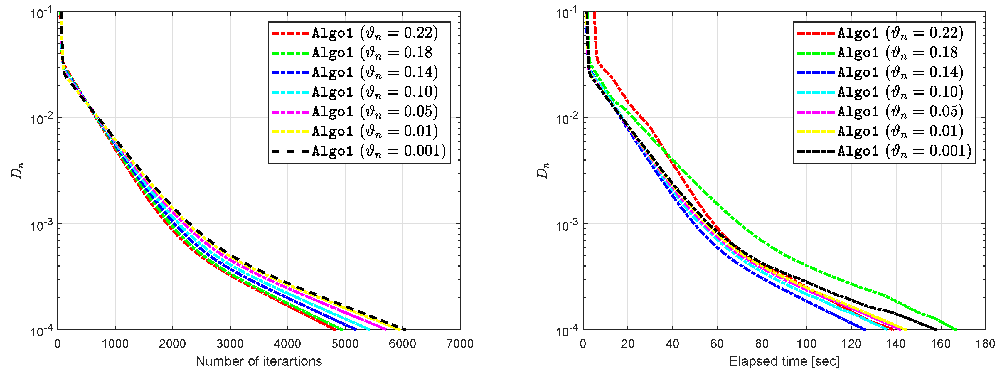
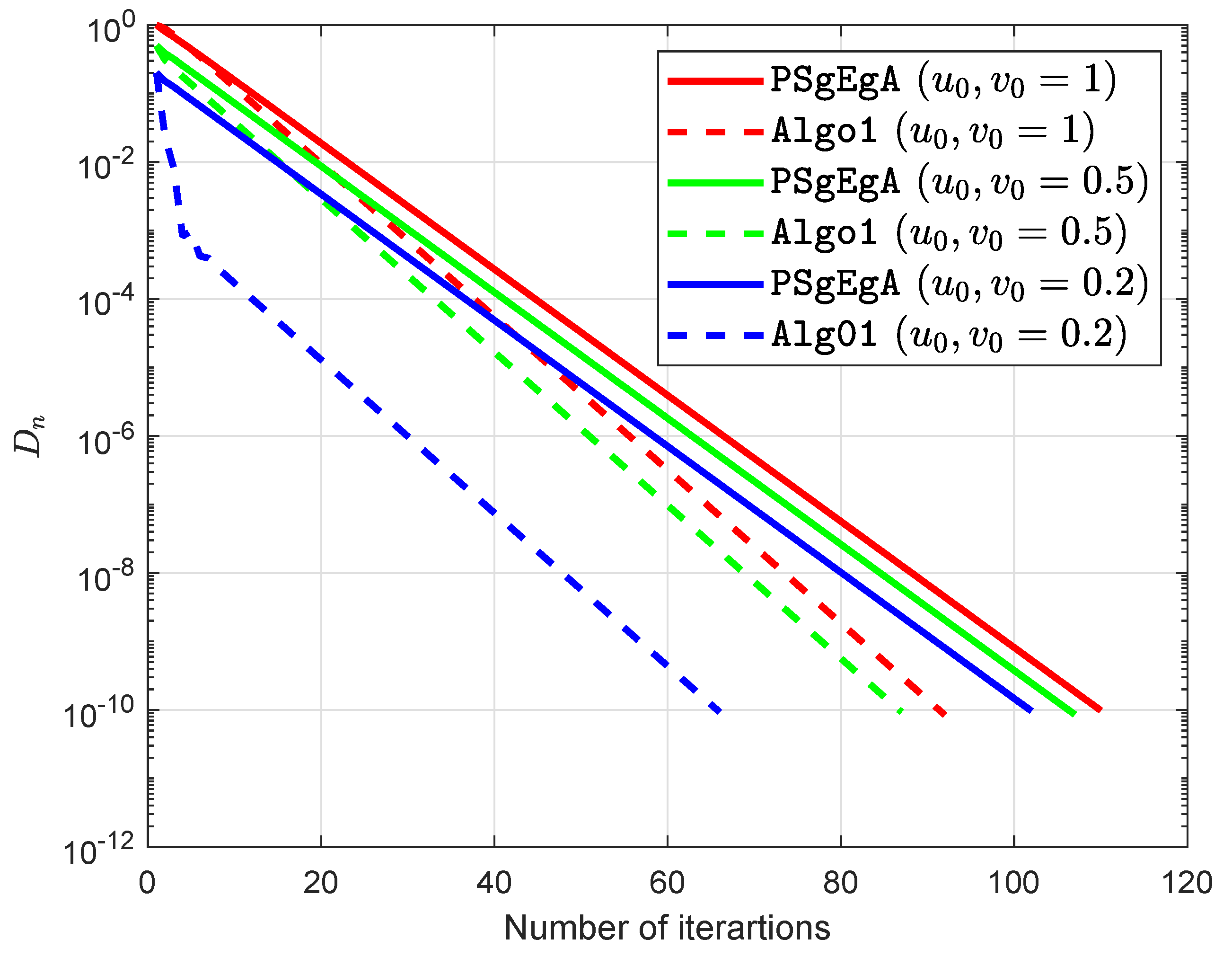
Remark 2.

For ${\vartheta }_n=\vartheta =0$ in Algorithm 1 gives the results as in [35,36].

4. Inertial Popov’s Two-Step Subgradient Extragradient Algorithm for Strongly Pseudomonotone EP

The second algorithm is also an inertial algorithm that is able to solve the strongly pseudomonotone equilibrium problem. However, the advantage of this algorithm is that there is no need for prior information regarding the strongly pseudomonotone constant $\gamma$ and Lipschitz constants $L_1,L_2$. Let $\left\{{\lambda }_n\right\}\subset (0,+\infty )$ be a non-increasing sequence, so that the following conditions are satisfied:

$$\left(\mathrm{T}1\right):\underset{n\to \infty }{lim}{\lambda }_n=0\mathrm{and}\left(\mathrm{T}2\right):\sum _{n=1}^{\infty }{\lambda }_n=+\infty .$$

(43)

Assumption 2.

Let a bifunction $f:\mathbb{E}\times \mathbb{E}\to \mathbb{R}$ satisfies the following conditions:

(B1)

$f(\tilde{u},\tilde{u})=0,\forall \tilde{u}\in K$ and f is strongly pseudomontone on K;

(B2)

f meet the Lipschitz-type condition on $\mathbb{E}$ with two positive constants $L_1$ and $L_2$;

(B3)

$f(\tilde{u},.)$ is sub-differentiable and convex on $\mathbb{E}$ for all $\tilde{u}\in \mathbb{E}.$

Lemma 11.

Assume that $f:\mathbb{E}\times \mathbb{E}\to \mathbb{R}$ satisfies the conditions (B1)–(B3). Let the solution set $SO{L}_{EP(f,K)}$ is nonempty. For each ${\xi }^{*}\in SO{L}_{EP(f,K)}$, we have

$$\begin{array}{cc}\hfill \parallel u_{n+1}-{\xi }^{*}{\parallel }^2& \le \parallel {\rho }_n-{\xi }^{*}{\parallel }^2-(1-4{\lambda }_n{L}_1)\parallel {\rho }_n-v_n{\parallel }^2-(1-2{\lambda }_n{L}_2){\parallel u_{n+1}-v_n\parallel }^2\hfill \\ \hfill & +4{\lambda }_n{L}_1\parallel {\rho }_n-v_{n-1}{\parallel }^2-2\gamma {\lambda }_n{\parallel v_n-{\xi }^{*}\parallel }^2.\hfill \end{array}$$

Now, we are in a position to provide our second convergence result of this work.

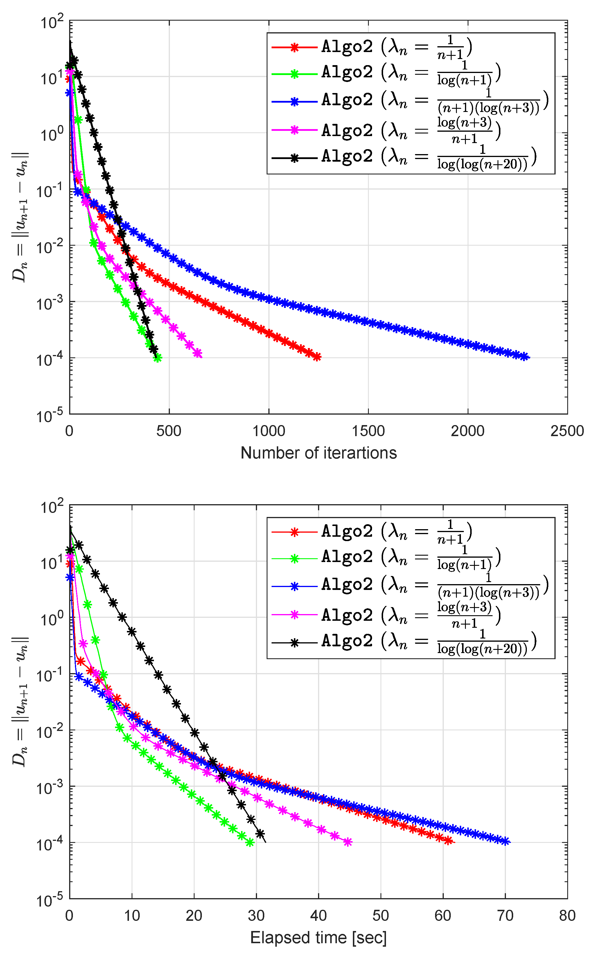
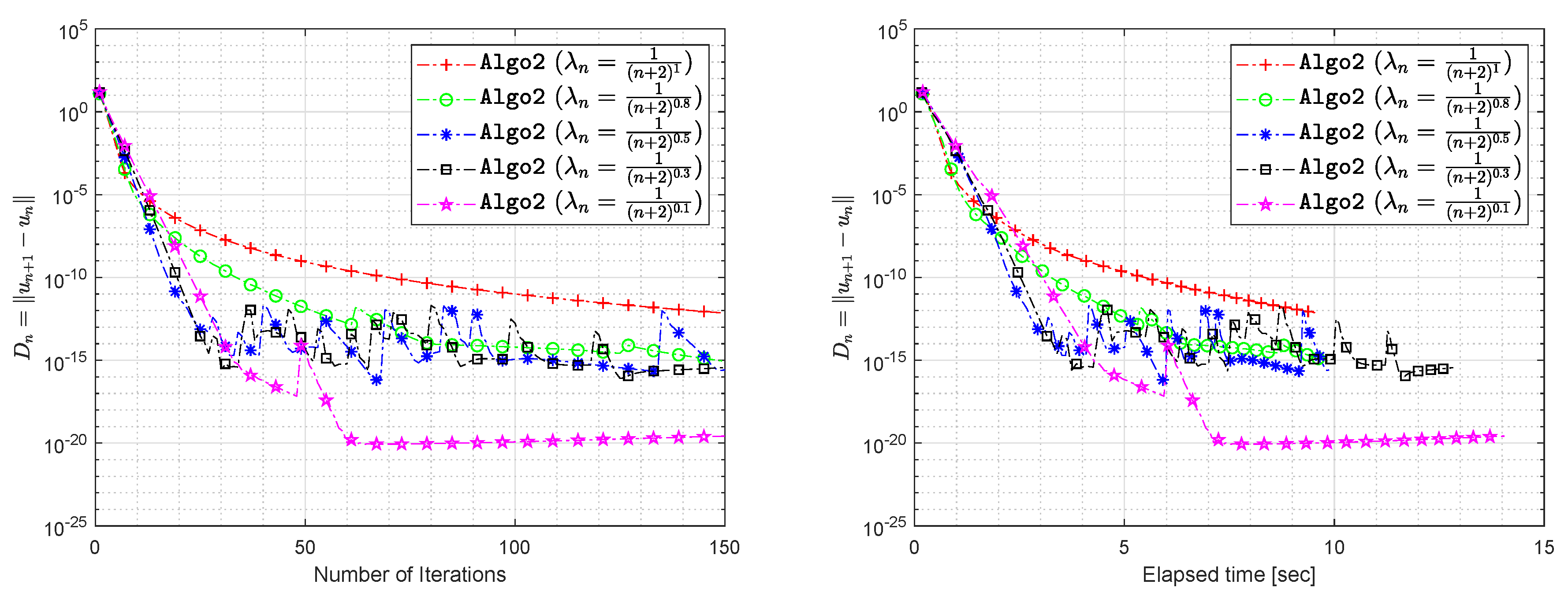
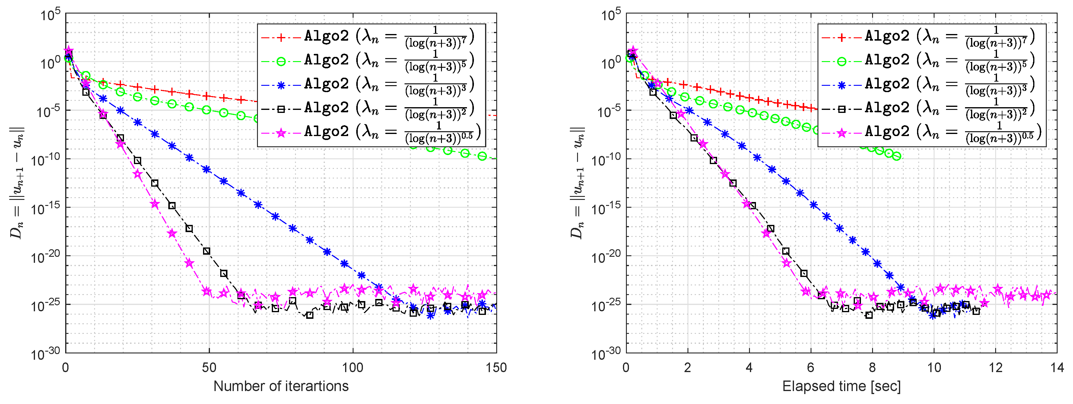
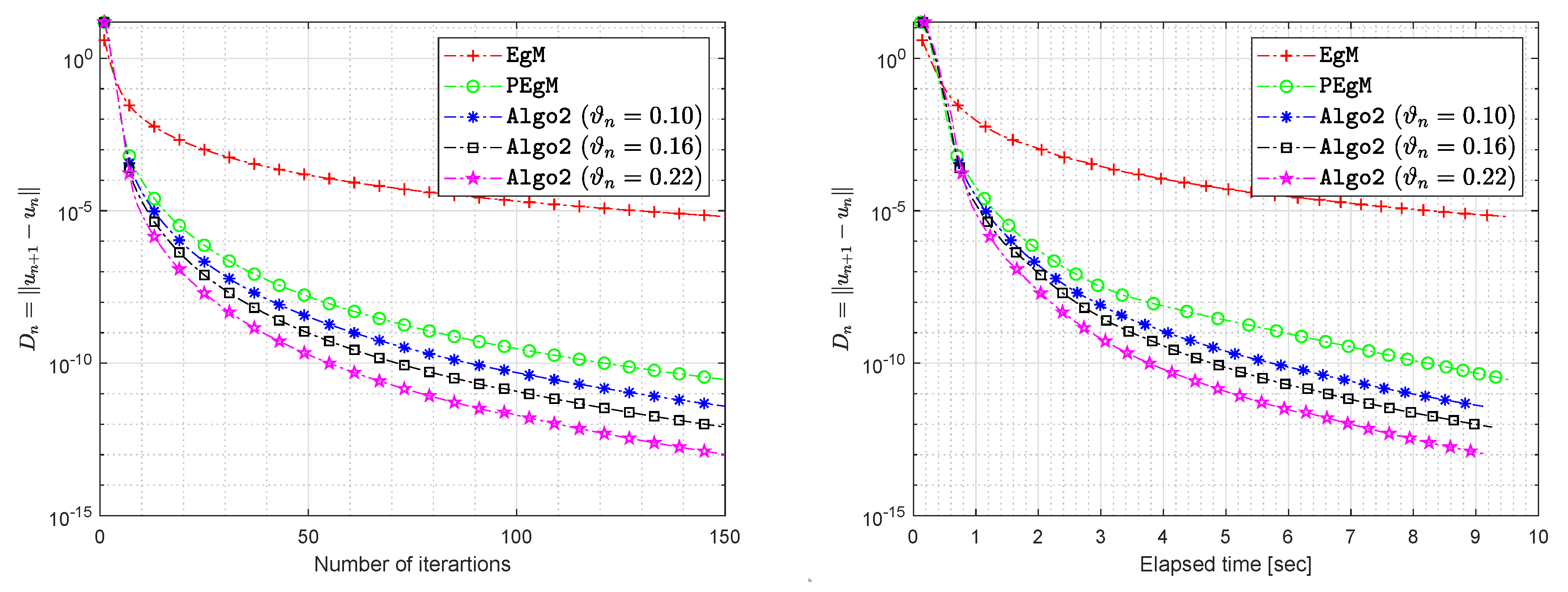
Theorem 2.

Assume that $f:\mathbb{E}\times \mathbb{E}\to \mathbb{R}$ satisfies the conditions (B1)–(B3). Let $\left\{u_n\right\}$, $\left\{v_n\right\}$ and $\left\{{\rho }_n\right\}$ are sequences in $\mathbb{E}$ generated by Algorithm 2 and ${\vartheta }_n$ is non-decreasing sequence with $0\le {\vartheta }_n\le \vartheta <\sqrt{5}-2$. Subsequently, $\left\{u_n\right\}$, $\left\{v_n\right\}$ and $\left\{{\rho }_n\right\}$ strongly converge to an element ${\xi }^{*}$ in $SO{L}_{EP(f,K)}$.

Algorithm 2 (Two-step Subgradient Extragradient Algorithm for Strongly Pseudomonotone EP)

Initialization: Choose $u_{-1},u_0,v_0\in \mathbb{E}$, $0\le {\vartheta }_n\le \vartheta <\sqrt{5}-2$ and a sequence $\left\{{\lambda }_n\right\}$ satisfying (43). Set $$u_1=\underset{}{argmin}\{{\lambda }_{0}f(v_0,y)+\frac{1}{2}\parallel {\rho }_0-y{\parallel }^2:y\in K\},$$ $$v_1=\arg \min \{{\lambda }_{1}f(v_0,y)+\frac{1}{2}\parallel {\rho }_1-y{\parallel }^2:y\in K\},$$ where ${\rho }_0=u_0+{\vartheta }_0(u_0-u_{-1})$ and ${\rho }_1=u_1+{\vartheta }_1(u_1-u_0)$. Iterative steps: Assume that $u_{n-1}$, $u_n$, $v_{n-1}$ and $v_n$ are known for $n\ge 1$ and $$H_n=\{z\in \mathbb{E}:\langle {\rho }_n-{\lambda }_n{\omega }_{n-1}-v_n,z-v_n\rangle \le 0\},$$ where ${\omega }_{n-1}\in \partial f(v_{n-1},v_n)$. Step 1: Compute $$u_{n+1}=\underset{}{argmin}\{{\lambda }_{n}f(v_n,y)+\frac{1}{2}\parallel {\rho }_n-y{\parallel }^2:y\in H_n\},$$ where ${\rho }_n=u_n+{\vartheta }_n(u_n-u_{n-1})$. Step 2: Compute $$v_{n+1}=\underset{}{argmin}\{{\lambda }_{n+1}f(v_n,y)+\frac{1}{2}\parallel {\rho }_{n+1}-y{\parallel }^2:y\in K\},$$ where ${\rho }_{n+1}=u_{n+1}+{\vartheta }_{n+1}(u_{n+1}-u_n)$. Step 3: If $u_{n+1}={\rho }_n$ and $v_n=v_{n-1}$, then STOP. Otherwise set $n:=n+1$ and go to Step 1.

Proof. 

The proof is the identical as the proof of Theorem 1, but there are still few changes. We provide the proof for the readable purpose. By Lemma 11 and adding $4L_1{\lambda }_n{\parallel {\rho }_{n+1}-v_n\parallel }^2$ in both sides, we have

$$\begin{array}{cc}\hfill & \parallel u_{n+1}-{\xi }^{*}{\parallel }^2+4L_1{\lambda }_n{\parallel {\rho }_{n+1}-v_n\parallel }^2\hfill \\ \hfill & \le \parallel {\rho }_n-{\xi }^{*}{\parallel }^2-(1-4L_1{\lambda }_n)\parallel {\rho }_n-v_n{\parallel }^2-(1-2L_2{\lambda }_n){\parallel u_{n+1}-v_n\parallel }^2\hfill \\ \hfill & +4L_1{\lambda }_n\parallel {\rho }_n-v_{n-1}{\parallel }^2-2\gamma {\lambda }_n\parallel v_n-{\xi }^{*}{\parallel }^2+4L_1{\lambda }_n{\parallel {\rho }_{n+1}-v_n\parallel }^2.\hfill \end{array}$$

(44)

By using the definition of ${\rho }_n$ in Algorithm 2, we have

$$\begin{array}{cc}\hfill \parallel {\rho }_n-{\xi }^{*}{\parallel }^2& =(1+{\vartheta }_n)\parallel u_n-{\xi }^{*}{\parallel }^2-{\vartheta }_n\parallel u_{n-1}-{\xi }^{*}{\parallel }^2+{\vartheta }_n(1+{\vartheta }_n){\parallel u_n-u_{n-1}\parallel }^2.\hfill \end{array}$$

(45)

By using the definition ${\rho }_{n+1}$ in Algorithm 2, we also have

$$\begin{array}{cc}\hfill \parallel {\rho }_{n+1}-v_n{\parallel }^2& \le (1+{\vartheta }_n)\parallel u_{n+1}-v_n{\parallel }^2+{\vartheta }_n(1+{\vartheta }_n){\parallel u_{n+1}-u_n\parallel }^2.\hfill \end{array}$$

(46)

Combining the expression (44)–(46), we obtain

$$\begin{array}{cc}\hfill & \parallel u_{n+1}-{\xi }^{*}{\parallel }^2+4L_1{\lambda }_{n+1}{\parallel {\rho }_{n+1}-v_n\parallel }^2\hfill \\ \hfill & \le (1+{\vartheta }_n)\parallel u_n-{\xi }^{*}{\parallel }^2-{\vartheta }_n\parallel u_{n-1}-{\xi }^{*}{\parallel }^2+{\vartheta }_n(1+{\vartheta }_n){\parallel u_n-u_{n-1}\parallel }^2\hfill \\ \hfill & +4L_1{\lambda }_n\parallel {\rho }_n-v_{n-1}{\parallel }^2-(1-4L_1{\lambda }_n)\parallel {\rho }_n-v_n{\parallel }^2-(1-2L_2{\lambda }_n){\parallel u_{n+1}-v_n\parallel }^2\hfill \\ \hfill & +4L_1{\lambda }_n(1+{\vartheta }_n)\parallel u_{n+1}-v_n{\parallel }^2+4L_1{\lambda }_n{\vartheta }_n(1+{\vartheta }_n)\parallel u_{n+1}-u_n{\parallel }^2-2\gamma {\lambda }_n{\parallel v_n-{\xi }^{*}\parallel }^2\hfill \end{array}$$

(47)

$$\begin{array}{cc}\hfill & \le (1+{\vartheta }_n)\parallel u_n-{\xi }^{*}{\parallel }^2-{\vartheta }_n\parallel u_{n-1}-{\xi }^{*}{\parallel }^2+4L_1{\lambda }_n{\parallel {\rho }_n-v_{n-1}\parallel }^2\hfill \\ \hfill & +{\vartheta }_n(1+{\vartheta }_n)\parallel u_n-u_{n-1}{\parallel }^2+4L_1{\lambda }_n(1+{\vartheta }_n)\parallel u_{n+1}-u_n{\parallel }^2-2\gamma {\lambda }_n{\parallel v_n-{\xi }^{*}\parallel }^2\hfill \\ \hfill & -\frac{\left(1-2L_2{\lambda }_n-4L_1{\lambda }_n(1+{\vartheta }_n)\right)}{2}\left[2(\parallel u_{n+1}-v_n{\parallel }^2+\parallel {\rho }_n-v_n{\parallel }^2)\right].\hfill \end{array}$$

(48)

Next, we let ${\varrho }_n=\frac{1-2L_2{\lambda }_n-4L_1{\lambda }_n(1+{\vartheta }_n)}{2}$ and

$${\mathsf{\Phi }}_n=\parallel u_n-{\xi }^{*}{\parallel }^2-{\vartheta }_n\parallel u_{n-1}-{\xi }^{*}{\parallel }^2+4L_1{\lambda }_n{\parallel {\rho }_n-v_{n-1}\parallel }^2.$$

Due to the above substituting the expression (48) turns into the following:

$$\begin{array}{cc}\hfill {\mathsf{\Phi }}_{n+1}& \le {\mathsf{\Phi }}_n+{\vartheta }_n(1+{\vartheta }_n)\parallel u_n-u_{n-1}{\parallel }^2+4L_1{\lambda }_n{\vartheta }_n(1+{\vartheta }_n){\parallel u_{n+1}-u_n\parallel }^2\hfill \\ \hfill & -{\varrho }_n\parallel u_{n+1}-{\rho }_n{\parallel }^2-2\gamma {\lambda }_n{\parallel v_n-{\xi }^{*}\parallel }^2,\hfill \end{array}$$

(49)

By the definition ${\rho }_{n+1}$, we have

$$\begin{array}{cc}\hfill \parallel u_{n+1}-{\rho }_n{\parallel }^2& \ge (1-{\vartheta }_n)\parallel u_{n+1}-u_n{\parallel }^2+({\vartheta }_n^2-{\vartheta }_n){\parallel u_n-u_{n-1}\parallel }^2.\hfill \end{array}$$

(50)

Combining the expression (49) and (50), we obtain

$$\begin{array}{cc}\hfill {\mathsf{\Phi }}_{n+1}& \le {\mathsf{\Phi }}_n+{\vartheta }_n(1+{\vartheta }_n)\parallel u_n-u_{n-1}{\parallel }^2+4L_1{\lambda }_n{\vartheta }_n(1+{\vartheta }_n){\parallel u_{n+1}-u_n\parallel }^2\hfill \\ \hfill & -2\gamma {\lambda }_n\parallel v_n-{\xi }^{*}{\parallel }^2-{\varrho }_n(1-{\vartheta }_n)\parallel u_{n+1}-u_n{\parallel }^2-{\varrho }_n({\vartheta }_n^2-{\vartheta }_n){\parallel u_n-u_{n-1}\parallel }^2\hfill \\ \hfill & ={\mathsf{\Phi }}_n+R_n\parallel u_n-u_{n-1}{\parallel }^2-Q_n\parallel u_{n+1}-u_n{\parallel }^2-2\gamma {\lambda }_n{\parallel v_n-{\xi }^{*}\parallel }^2,\hfill \end{array}$$

(51)

where $R_n:={\vartheta }_n(1+{\vartheta }_n)+{\varrho }_n{\vartheta }_n(1-{\vartheta }_n)$ and $Q_n:={\varrho }_n(1-{\vartheta }_n)-4L_1{\lambda }_n{\vartheta }_n(1+{\vartheta }_n).$ In addition, we also take ${\mathsf{\Psi }}_n={\mathsf{\Phi }}_n+R_n{\parallel u_n-u_{n-1}\parallel }^2.$ It follows from (51) that

$${\mathsf{\Psi }}_{n+1}-{\mathsf{\Psi }}_n\le -(Q_n-R_{n+1})\parallel u_{n+1}-u_n{\parallel }^2-2\gamma {\lambda }_n{\parallel v_n-{\xi }^{*}\parallel }^2.$$

(52)

Since ${\lambda }_n\to 0$, then there exists a finite number $n_0\in \mathbb{N}$ such that

$$0<{\lambda }_n<\frac{\frac{1}{2}-2\vartheta -\frac{1}{2}{\vartheta }^2}{L_2{(1-\vartheta )}^2+2L_1(1+\vartheta +{\vartheta }^2+{\vartheta }^3)},n\ge n_0.$$

Similarly, it follows from (24) and expression (52) implies that

$${\mathsf{\Psi }}_{n+1}-{\mathsf{\Psi }}_n\le -\delta {\parallel u_{n+1}-u_n\parallel }^2\le 0,n\ge n_0.$$

(53)

The above implies that the sequence $\left\{{\mathsf{\Psi }}_n\right\}$ is non-increasing for $n\ge n_0.$ From the value of ${\mathsf{\Psi }}_n$, we have

$$\begin{array}{cc}\hfill \parallel u_n-{\xi }^{*}{\parallel }^2& \le {\mathsf{\Psi }}_n+{\vartheta }_n{\parallel u_{n-1}-{\xi }^{*}\parallel }^2\hfill \\ \hfill & \le {\mathsf{\Psi }}_{n_0}+\vartheta {\parallel u_{n-1}-{\xi }^{*}\parallel }^2\hfill \\ \hfill & \le \cdots \le {\mathsf{\Psi }}_{n_0}({\vartheta }^{n-n_0}+\cdots +1)+{\vartheta }^{n-n_0}{\parallel u_{n_0}-{\xi }^{*}\parallel }^2\hfill \\ \hfill & \le \frac{{\mathsf{\Psi }}_{n_0}}{1-\vartheta }+{\vartheta }^{n-n_0}{\parallel u_{n_0}-{\xi }^{*}\parallel }^2.\hfill \end{array}$$

(54)

From the definition of ${\mathsf{\Psi }}_{n+1}$ with the expression (54), we obtain

$$\begin{array}{cc}\hfill -{\mathsf{\Psi }}_{n+1}& \le {\vartheta }_{n+1}{\parallel u_n-{\xi }^{*}\parallel }^2\hfill \\ \hfill & \le \vartheta \parallel u_n-{\xi }^{*}{\parallel }^2\hfill \\ \hfill & \le \vartheta \frac{{\mathsf{\Psi }}_{n_0}}{1-\vartheta }+{\vartheta }^{n-n_0+1}{\parallel u_{n_0}-{\xi }^{*}\parallel }^2\hfill \\ \hfill & \le \vartheta \frac{{\mathsf{\Psi }}_{n_0}}{1-\vartheta }+{\parallel u_{n_0}-{\xi }^{*}\parallel }^2.\hfill \end{array}$$

(55)

It is follows from (53) and (55) that

$$\begin{array}{cc}\hfill \delta \sum _{n=n_0}^k{\parallel u_{n+1}-u_n\parallel }^2& \le {\mathsf{\Psi }}_{n_0}-{\mathsf{\Psi }}_{k+1}\hfill \\ \hfill & \le {\mathsf{\Psi }}_{n_0}+\vartheta \frac{{\mathsf{\Psi }}_{n_0}}{1-\vartheta }+{\parallel u_{n_0}-{\xi }^{*}\parallel }^2\hfill \\ \hfill & \le \frac{{\mathsf{\Psi }}_{n_0}}{1-\vartheta }+{\parallel u_{n_0}-{\xi }^{*}\parallel }^2,\hfill \end{array}$$

(56)

letting $k\to \infty$ in the expression (56), we obtain

$$\sum _{n=1}^{\infty }\parallel u_{n+1}-u_n{\parallel }^2<+\infty \mathrm{implies}\mathrm{that}\parallel u_{n+1}-u_n\parallel \to 0\mathrm{as}n\to \infty .$$

(57)

From the expression (20) and (57), we obtain

$$\parallel u_{n+1}-{\rho }_n\parallel \to 0\mathrm{as}n\to \infty .$$

(58)

The expression (55) implies that

$$-{\mathsf{\Phi }}_{n+1}\le \vartheta \frac{{\mathsf{\Psi }}_{n_0}}{1-\vartheta }+\parallel u_{n_0}-{\xi }^{*}{\parallel }^2+R_{n+1}{\parallel u_{n+1}-u_n\parallel }^2.$$

(59)

It follows from (48) for all $n\ge n_0$, such that

$$\begin{array}{cc}\hfill & \left(1-2L_2{\lambda }_n-4L_1{\lambda }_n(1+\vartheta )\right)\left[\parallel u_{n+1}-v_n{\parallel }^2+{\parallel {\rho }_n-v_n\parallel }^2\right]\hfill \\ \hfill & \le {\mathsf{\Phi }}_n-{\mathsf{\Phi }}_{n+1}+\vartheta (1+\vartheta )\parallel u_n-u_{n-1}{\parallel }^2+4L_1{\lambda }_n\vartheta (1+\vartheta ){\parallel u_{n+1}-u_n\parallel }^2.\hfill \end{array}$$

(60)

Consider the expression (60) for $n_0,n_0+1,\cdots ,k.$ Summing them up, we obtain

$$\begin{array}{cc}\hfill & \left(1-2L_2{\lambda }_n-4L_1{\lambda }_n(1+\vartheta )\right)\sum _{n=n_0}^k\left[\parallel u_{n+1}-v_n{\parallel }^2+{\parallel {\rho }_n-v_n\parallel }^2\right]\hfill \\ \hfill & \le {\mathsf{\Phi }}_{n_0}-{\mathsf{\Phi }}_{k+1}+\vartheta (1+\vartheta )\sum _{n=n_0}^k\parallel u_n-u_{n-1}{\parallel }^2+\frac{4L_1}{2L_2+4L_1}\vartheta (1+\vartheta )\sum _{n=n_0}^k{\parallel u_{n+1}-u_n\parallel }^2\hfill \\ \hfill & \le {\mathsf{\Phi }}_{n_0}+\vartheta \frac{{\mathsf{\Phi }}_{n_0}}{1-\vartheta }+\parallel u_{n_0}-{\xi }^{*}{\parallel }^2+R_{k+1}{\parallel u_{k+1}-u_k\parallel }^2\hfill \\ \hfill & +\vartheta (1+\vartheta )\sum _{n=n_0}^k\parallel u_n-u_{n-1}{\parallel }^2+\frac{4L_1}{2L_2+4L_1}\vartheta (1+\vartheta )\sum _{n=n_0}^k{\parallel u_{n+1}-u_n\parallel }^2\hfill \\ \hfill & =\frac{{\mathsf{\Phi }}_{n_0}}{1-\vartheta }+\parallel u_{n_0}-{\xi }^{*}{\parallel }^2+R_{k+1}{\parallel u_{k+1}-u_k\parallel }^2\hfill \\ \hfill & +\vartheta (1+\vartheta )\sum _{n=n_0}^k\parallel u_n-u_{n-1}{\parallel }^2+\frac{4L_1}{2L_2+4L_1}\vartheta (1+\vartheta )\sum _{n=n_0}^k{\parallel u_{n+1}-u_n\parallel }^2,\hfill \end{array}$$

(61)

By letting $k\to \infty$ in the expression (61) implies that

$$\sum _n\parallel u_{n+1}-v_n{\parallel }^2<+\infty \mathrm{and}\sum _n{\parallel {\rho }_n-v_n\parallel }^2<+\infty ,$$

(62)

and

$$\underset{n\to \infty }{lim}\parallel u_{n+1}-v_n\parallel =\underset{n\to \infty }{lim}\parallel {\rho }_n-v_n\parallel =0.$$

(63)

We can easily derive the following relationship:

$$\underset{n\to \infty }{lim}\parallel u_n-v_n\parallel =\underset{n\to \infty }{lim}\parallel u_n-{\rho }_n\parallel =\underset{n\to \infty }{lim}\parallel v_{n-1}-v_n\parallel =0.$$

(64)

By using the value ${\rho }_n$, we obtain

$$\begin{array}{cc}\hfill \parallel {\rho }_n-v_{n-1}{\parallel }^2& \le (1+\vartheta )\parallel u_n-v_{n-1}{\parallel }^2+\vartheta (1+\vartheta ){\parallel u_n-u_{n-1}\parallel }^2.\hfill \end{array}$$

(65)

Now, summing up equation (65) for $n=n_0,n_0+1\cdots ,k$, we obtain

$$\sum _{n=n_0}^k\parallel {\rho }_n-v_{n-1}{\parallel }^2\le (1+\vartheta )\sum _{n=n_0}^k\parallel u_n-v_{n-1}{\parallel }^2+\vartheta (1+\vartheta )\sum _{n=n_0}^k{\parallel u_n-u_{n-1}\parallel }^2$$

(66)

The above expression with (57) and (62) implies that

$$\sum _{n=1}^{\infty }{\parallel {\rho }_n-v_{n-1}\parallel }^2<+\infty .$$

(67)

Furthermore, the expression (47) gives that

$$\begin{array}{cc}\hfill & \parallel u_{n+1}-{\xi }^{*}{\parallel }^2\hfill \\ \hfill & \le (1+\vartheta )\parallel u_n-{\xi }^{*}{\parallel }^2-\vartheta \parallel u_{n-1}-{\xi }^{*}{\parallel }^2+\vartheta (1+\vartheta )\parallel u_n-u_{n-1}{\parallel }^2+4L_1{\lambda }_n{\parallel {\rho }_n-v_{n-1}\parallel }^2.\hfill \end{array}$$

(68)

The above expression through (57), (67), and Lemma 4 implies that

$$\underset{n\to \infty }{lim}\parallel u_n-{\xi }^{*}\parallel =l.$$

(69)

The expression (64) with (69), we obtain

$$\underset{n\to \infty }{lim}\parallel {\rho }_n-{\xi }^{*}\parallel =\underset{n\to \infty }{lim}\parallel v_n-{\xi }^{*}\parallel =l.$$

(70)

Now, we are showing that the sequence $\left\{u_n\right\}$ converges strongly to ${\xi }^{*}.$ Due to the condition on ${\lambda }_n$ for all $n\ge n_0$, we can easily observe the following inequality:

$$0<{\lambda }_n<\frac{1}{2L_2+4L_1},\forall n\ge n_0.$$

It follows from Lemma 11, such that

$$2\gamma {\lambda }_n\parallel v_n-{\xi }^{*}{\parallel }^2\le \parallel {\rho }_n-{\xi }^{*}{\parallel }^2-\parallel u_{n+1}-{\xi }^{*}{\parallel }^2+4L_1{\lambda }_n{\parallel {\rho }_n-v_{n-1}\parallel }^2,\forall n\ge n_0.$$

(71)

From the expression (45) and (71), we obtain

$$\begin{array}{cc}\hfill 2\gamma {\lambda }_n{\parallel v_n-{\xi }^{*}\parallel }^2& \le -\parallel u_{n+1}-{\xi }^{*}{\parallel }^2+(1+{\vartheta }_n)\parallel u_n-{\xi }^{*}{\parallel }^2-{\vartheta }_n{\parallel u_{n-1}-{\xi }^{*}\parallel }^2\hfill \\ & +{\vartheta }_n(1+{\vartheta }_n)\parallel u_n-u_{n-1}{\parallel }^2+4L_1{\lambda }_n{\parallel {\rho }_n-v_{n-1}\parallel }^2\hfill \\ \hfill & \le (\parallel u_n-{\xi }^{*}{\parallel }^2-\parallel u_{n+1}-{\xi }^{*}{\parallel }^2)+2\vartheta \parallel u_n-u_{n-1}{\parallel }^2\hfill \\ \hfill & +({\vartheta }_n\parallel u_n-{\xi }^{*}{\parallel }^2-{\vartheta }_{n-1}\parallel u_{n-1}-{\xi }^{*}{\parallel }^2)+4L_1{\lambda }_n{\parallel {\rho }_n-v_{n-1}\parallel }^2.\hfill \end{array}$$

(72)

It follows from expression (72) that

$$\begin{array}{c}\sum _{n=n_0}^{k}2\gamma {\lambda }_n{\parallel v_n-{\xi }^{*}\parallel }^2\hfill \\ \le (\parallel u_{n_0}-{\xi }^{*}{\parallel }^2-\parallel u_{k+1}-{\xi }^{*}{\parallel }^2)+2\vartheta \sum _{n=n_0}^k{\parallel u_n-u_{n-1}\parallel }^2\hfill \\ +({\vartheta }_k\parallel u_k-{\xi }^{*}{\parallel }^2-{\vartheta }_{n_0-1}\parallel u_{n_0-1}-{\xi }^{*}{\parallel }^2)+\frac{4L_1}{2L_2+4L_1}\sum _{n=n_0}^k{\parallel {\rho }_n-v_{n-1}\parallel }^2\hfill \\ \le \parallel u_{n_0}-{\xi }^{*}{\parallel }^2+\vartheta \parallel u_k-{\xi }^{*}{\parallel }^2+2\vartheta \sum _{n=n_0}^k\parallel u_n-u_{n-1}{\parallel }^2+\frac{4L_1}{2L_2+4L_1}\sum _{n=n_0}^k{\parallel {\rho }_n-v_{n-1}\parallel }^2\hfill \\ \le M,\hfill \end{array}$$

(73)

for $M\ge 0.$ It implies that

$$\sum _{n=1}^{\infty }2\gamma {\lambda }_n{\parallel v_n-{\xi }^{*}\parallel }^2<+\infty .$$

(74)

By the Lemma 2 and (74) implies that

$$lim\; inf\parallel v_n-{\xi }^{*}\parallel =0.$$

(75)

Finally, expression (69) and (75) provide that ${lim}_{n\to \infty }\parallel u_n-{\xi }^{*}\parallel =0.$ This completes the proof. □

5. Application to Variational Inequality Problems

For considering Algorithm 1 and Theorem 1, we can able to write the next result for solving variational inequality problems that involve pseudomonotone and Lipschitz continuous operator.

Corollary 1.

Assume that $H:K\to \mathbb{E}$ be a Lipschitz continuous with the constant L and pseudomonotone operator. Let $\left\{u_n\right\}$, $\left\{v_n\right\}$ and $\left\{{\rho }_n\right\}$ be sequences generated, as follows:

(i)

Choose $u_{-1},u_0,v_0\in \mathbb{E}$, $0\le {\vartheta }_n\le \vartheta <\sqrt{5}-2$ and $\lambda (\vartheta ,L_1,L_2)>0.$ Compute

$$\left\{\begin{array}{c}{u}_1=P_K({\rho }_0-\lambda H{v}_0),\mathit{where}{\rho }_0=u_0+{\vartheta }_0(u_0-u_{-1}),\hfill \\ v_1=P_K({\rho }_1-\lambda H{v}_0),\mathit{where}{\rho }_1=u_1+{\vartheta }_1(u_1-u_0).\hfill \end{array}\right.$$

(ii)

Given $u_{n-1},u_n$, $v_{n-1},$ and $v_n$ for each $n\ge 1,$ and construct the half-space first as

$$H_n=\{z\in \mathbb{E}:\langle {\rho }_n-\lambda H{v}_{n-1}-v_n,z-v_n\rangle \le 0\}.$$

(iii)

Evaluate

$$\left\{\begin{array}{c}{u}_{n+1}=P_{H_n}({\rho }_n-\lambda H{v}_n),\mathit{where}{\rho }_n=u_n+{\vartheta }_n(u_n-u_{n-1}),\hfill \\ v_{n+1}=P_K({\rho }_{n+1}-\lambda H{v}_n),\mathit{where}{\rho }_{n+1}=u_{n+1}+{\vartheta }_{n+1}(u_{n+1}-u_n),\hfill \end{array}\right.$$

where $\lambda >0$, such that

$$0<\lambda <\frac{\frac{1}{2}-2\vartheta -\frac{1}{2}{\vartheta }^2}{L_2{(1-\vartheta )}^2+2L_1(1+\vartheta +{\vartheta }^2+{\vartheta }^3)}\mathit{and}0\le {\vartheta }_n\le \vartheta <\sqrt{5}-2,$$

with $L_1=L_2=\frac{L}{2}$. Subsequently, sequence $\left\{u_n\right\}$, $\left\{{\rho }_n\right\}$ and $\left\{v_n\right\}$ converge weakly to ${\xi }^{*}\in SO{L}_{VI(H,K)}$.

From the consideration on Algorithm 2 and Theorem 2, we state the following result for the class of variational inequality problems involving strongly pseudomonotone and Lipschitz continuous operator.

Corollary 2.

Assume that $H:K\to \mathbb{E}$ is a Lipschitz continuous and strongly pseudomonotone operator with the constant $L$. Let $\left\{u_n\right\}$, $\left\{v_n\right\}$ and $\left\{{\rho }_n\right\}$ are the sequences generated as follows:

(i)

Choose $u_{-1},u_0,v_0\in \mathbb{E}$, $0\le {\vartheta }_n\le \vartheta <\sqrt{5}-2$ and a sequence $\left\{{\lambda }_n\right\}$ satisfying (43). Compute

$$\left\{\begin{array}{c}{u}_1=P_K({\rho }_0-{\lambda }_{0}H{v}_0),\mathit{where}{\rho }_0=u_0+{\vartheta }_0(u_0-u_{-1}),\hfill \\ v_1=P_K({\rho }_1-{\lambda }_{1}H{v}_0),\mathit{where}{\rho }_1=u_1+{\vartheta }_1(u_1-u_0).\hfill \end{array}\right.$$

(ii)

Given $u_{n-1},u_n$, $v_{n-1},$ and $v_n$ create a half space for each $n\ge 1,$ such that

$$H_n=\{z\in \mathbb{E}:\langle {\rho }_n-{\lambda }_{n}H{v}_{n-1}-v_n,z-v_n\rangle \le 0\}.$$

(iii)

Compute

$$\left\{\begin{array}{c}{u}_{n+1}=P_{H_n}({\rho }_n-{\lambda }_{n}H{v}_n),\mathit{where}{\rho }_n=u_n+{\vartheta }_n(u_n-u_{n-1}),\hfill \\ v_{n+1}=P_K({\rho }_{n+1}-{\lambda }_{n+1}H{v}_n),\mathit{where}{\rho }_{n+1}=u_{n+1}+{\vartheta }_{n+1}(u_{n+1}-u_n),\hfill \end{array}\right.$$

where $0\le {\vartheta }_n\le \vartheta <\sqrt{5}-2$, with $L_1=L_2=\frac{L}{2}$. The sequence $\left\{u_n\right\}$, $\left\{{\rho }_n\right\}$ and $\left\{v_n\right\}$ converge strongly to ${\xi }^{*}\in SO{L}_{VI(H,K)}$.

6. Computational Experiment

Some numerical results will be presented in this section to show the performance of our proposed methods. The MATLAB codes run in MATLAB version 9.5 (R2018b) on a PC (with Intel(R) Core(TM)i3-4010U CPU @ 1.70GHz 1.70GHz, RAM 4.00 GB).

6.1. Nash-Cournot Equilibrium Model of Electricity Markets

The Nash–Cournot equilibrium model of electricity markets in [20] is considered in this example. Assume that there are three companies $(i=1,2,3)$ generating electricity. These three companies has generating units denoted as $U_1=\left\{1\right\}$, $U_2=\{2,3\}$ and $U_3=\{4,5,6\}$, respectively. Let $u_j$ denote the generating power of the each unit for $i=\{1,2,3,4,5,6\}.$ Next, we take the electricity price P as $P=378.4-2{\sum }_{j=1}^6{u}_j.$ The cost of generating the j unit is written as:

$$c_j\left(u_j\right):=max\{\stackrel{\circ }{c_j}\left(u_j\right),\stackrel{•}{c_j}\left(u_j\right)\},$$

where $\stackrel{\circ }{c_j}\left(u_j\right):=\frac{\stackrel{\circ }{{\alpha }_j}}{2}{u}_j^2+\stackrel{\circ }{{\beta }_j}{u}_j+\stackrel{\circ }{{\gamma }_j}$ and $\stackrel{•}{c_j}\left(u_j\right):=\stackrel{•}{{\alpha }_j}{u}_j+\frac{\stackrel{•}{{\beta }_j}}{\stackrel{•}{{\beta }_j}+1}{\stackrel{•}{{\gamma }_j}}^{\frac{-1}{\stackrel{•}{{\beta }_j}}}{\left(u_j\right)}^{\frac{(\stackrel{•}{{\beta }_j}+1)}{\stackrel{•}{{\beta }_j}}}.$

Table 1. The values of parameters are used in the cost function.

j	$\stackrel{\circ }{{\mathit{\alpha }}_{\mathit{j}}}$	$\stackrel{\circ }{{\mathit{\beta }}_{\mathit{j}}}$	$\stackrel{\circ }{{\mathit{\gamma }}_{\mathit{j}}}$	$\stackrel{•}{{\mathit{\alpha }}_{\mathit{j}}}$	$\stackrel{•}{{\mathit{\beta }}_{\mathit{j}}}$	$\stackrel{•}{{\mathit{\gamma }}_{\mathit{j}}}$
1	0.0400	2.00	0.00	2.0000	1.0000	25.0000
2	0.0350	1.75	0.00	1.7500	1.0000	28.5714
3	0.1250	1.00	0.00	1.0000	1.0000	8.0000
4	0.0116	3.25	0.00	3.2500	1.0000	86.2069
5	0.0500	3.00	0.00	3.0000	1.0000	20.0000
6	0.0500	3.00	0.00	3.0000	1.0000	20.0000

provides the values of the unknown parameters. Consider that the profit of the firm i is

$$F_i\left(u\right):=P\sum _{j\in I_i}{u}_j-\sum _{j\in I_i}{c}_j\left(u_j\right)=\left(378.4-2\sum _{l=1}^6{u}_l\right)\sum _{j\in I_i}{u}_j-\sum _{j\in I_i}{c}_j\left(u_j\right),$$

with $u={(u_1,\cdots ,u_6)}^T$ corresponding to the constraint set $u\in C:=\{u\in {\mathbb{R}}^6:u_j^{min}\le u_j\le u_j^{max}\}$, with $u_j^{min}$ and $u_j^{max}$ values given in

Table 2. The parameter values use for constraint set.

j	1	2	3	4	5	6
$u_j^{min}$	0	0	0	0	0	0
$u_j^{max}$	80	80	50	55	30	40

. Consider the equilibrium function f by

$$f(u,v):=\sum _{i=1}^3\left({\varphi }_i(u,u)-{\varphi }_i(u,v)\right),$$

where

$${\varphi }_i(u,v):=\left[378.4-2\left(\sum _{j\notin I_i}{u}_j+\sum _{j\in I_i}{v}_j\right)\right]\sum _{j\in I_i}{v}_j-\sum _{j\in I_i}{c}_j\left(v_j\right).$$

The Nash–Cournot equilibrium models of electricity markets can be seen as an equilibrium problem in the following way (see [44] for more details):

$$\mathrm{Find}{\xi }^{*}\in K\mathrm{such}\mathrm{that}f({\xi }^{*},y)\ge 0,\forall y\in K.$$

During the numerical example in Section 6.1, we take the values $u_{-1}={(10,10,20,17,8,14)}^T$, $u_0={(10,20,30,10,0,1)}^T$, $v_0={(48,48,30,27,18,24)}^T$.

6.1.1. Algorithm 1 Behaviour for Different Values of ${\vartheta }_n$:

Figure 1 and

Table 3. Experiment in Section 6.1.1: Algorithm 1 performance for varying parameters extrapolation factor ${\vartheta }_n$.

Algo.name	${\mathit{\vartheta }}_{\mathit{n}}$	$\mathit{\lambda }$	${\mathit{\xi }}^{*}$	Iter.	Time	TOL
Algo1	0.22	0.02	${(46.6525,32.1462,15.0018,25.0170,10.8987,10.8982)}^T$	4824	138.915365	${10}^{-4}$
Algo1	0.18	0.02	${(46.6525,32.1460,15.0020,25.0104,10.9019,10.9016)}^T$	4949	166.620335	${10}^{-4}$
Algo1	0.14	0.02	${(46.6525,32.1460,15.0020,25.0035,10.9050,10.9053)}^T$	5193	127.834772	${10}^{-4}$
Algo1	0.10	0.02	${(46.6726,32.1460,15.0020,24.9969,10.9080,10.9089)}^T$	5432	136.310422	${10}^{-4}$
Algo1	0.05	0.02	${(46.6526,32.1460,15.0020,24.9885,10.9118,10.9134)}^T$	5721	142.108161	${10}^{-4}$
Algo1	0.01	0.02	${(46.6526,32.1460,15.0020,24.9818,10.9149,10.9170)}^T$	5945	144.356535	${10}^{-4}$
Algo1	0.001	0.02	${(46.6726,32.1460,15.0021,24.9787,10.9163,10.9187)}^T$	6043	157.711757	${10}^{-4}$

characterize the behaviour of error term $D_n=\parallel u_{n+1}-u_n\parallel \le TOL$ regarding Algorithm 1 (Algo1) with respect to different values of ${\vartheta }_n$ in terms of the number of iterations and elapsed time, respectively.

6.1.2. Algorithm 1 Comparison with Existing Algorithms

Figure 2 and

Table 4. Experiment in Section 6.1.2: Algorithm 1 comparison with existing algorithms using two different values of ${\vartheta }_n$.

Algo.name	${\mathit{\vartheta }}_{\mathit{n}}$	$\mathit{\lambda }$	${\mathit{\xi }}^{*}$	Iter.	Time	TOL
EgA	–	0.02	${(46.6526,32.1469,15.0012,24.9783,10.9154,10.9200)}^T$	7180	264.156236	${10}^{-4}$
PEgA	–	0.02	${(46.6526,32.1460,15.0021,24.9784,10.8164,10.9188)}^T$	6055	210.681669	${10}^{-4}$
PSgEgA	–	0.02	${(46.6525,32.1463,15.0017,25.0004,10.9058,10.9076)}^T$	5515	175.840493	${10}^{-4}$
Algo1	0.12	0.02	${(46.6725,32.1463,15.0017,25.0181,10.8976,10.8982)}^T$	4894	134.245610	${10}^{-4}$
Algo1	0.20	0.02	${(46.6725,32.1463,15.0017,25.0326,10.8910,10.8904)}^T$	4333	115.599023	${10}^{-4}$

explain the numerical comparison between Algorithm 1 (EgA) in [19], Algorithm 1 (PEgA) in [21], Algorithm 3.1 (PSgEgA) in [35,36] and Algorithm 1(Algo1).

Algorithm 1 (EgA) in [19]: Choose $u_0\in \mathbb{E}$ and $0<\lambda <min\{\frac{1}{2L_1},\frac{1}{2L_2}\}$.

$$\left\{\begin{array}{c}{v}_n=\underset{}{argmin}\{\lambda f(u_n,y)+\frac{1}{2}\parallel u_n-y{\parallel }^2:y\in K\},\hfill \\ u_{n+1}=\underset{}{argmin}\{\lambda f(v_n,y)+\frac{1}{2}\parallel u_n-y{\parallel }^2:y\in K\}.\hfill \end{array}\right.$$

(76)

Algorithm 1 (PEgA) in [21]: Choose $u_0,v_0\in \mathbb{E}$ and $0<\lambda <min\frac{1}{2L_2+4L_1}$.

$$\left\{\begin{array}{c}{u}_{n+1}=\underset{}{argmin}\{\lambda f(v_n,y)+\frac{1}{2}\parallel u_n-y{\parallel }^2:y\in K\},\hfill \\ v_{n+1}=\underset{}{argmin}\{\lambda f(v_n,y)+\frac{1}{2}\parallel u_{n+1}-y{\parallel }^2:y\in K\}.\hfill \end{array}\right.$$

(77)

Algorithm 3.1 (PSgEgA) in [35,36]: Choose $u_0,v_0\in \mathbb{E}$ and $0<\lambda <min\frac{1}{2L_2+4L_1}$.

(i)

$$\left\{\begin{array}{c}{u}_1=\underset{}{argmin}\{\lambda f(v_0,y)+\frac{1}{2}\parallel u_0-y{\parallel }^2:y\in K\},\hfill \\ v_1=\underset{}{argmin}\{\lambda f(v_0,y)+\frac{1}{2}\parallel u_1-y{\parallel }^2:y\in K\}.\hfill \end{array}\right.$$

(ii)

Given $u_{n-1},u_n$, $v_{n-1}$, $v_n$ for $n\ge 1$ and construct a half space as

$$H_n=\{z\in \mathbb{E}:\langle u_n-\lambda {\omega }_{n-1}-v_n,z-v_n\rangle \le 0\},\mathrm{where}{\omega }_{n-1}\in \partial f(v_{n-1},v_n).$$

(iii)

$$\left\{\begin{array}{c}{u}_{n+1}=\underset{}{argmin}\{\lambda f(v_n,y)+\frac{1}{2}\parallel u_n-y{\parallel }^2:y\in H_n\},\hfill \\ v_{n+1}=\underset{}{argmin}\{\lambda f(v_n,y)+\frac{1}{2}\parallel u_{n+1}-y{\parallel }^2:y\in K\}.\hfill \end{array}\right.$$

(78)

6.1.3. Algorithm 2 Behaviour by Using Different Step-Size Sequences ${\lambda }_n$

Figure 3 and

Table 5. Experiment in Section 6.1.3: Algorithm 2 numerical values by using different step-size sequences ${\lambda }_n$.

Algo.name	${\mathit{\vartheta }}_{\mathit{n}}$	$\mathit{\lambda }$	${\mathit{\xi }}^{*}$	Iter.	Time	TOL
Algo2	0.12	$\frac{1}{n+1}$	${(46.6526,32.1467,15.0011,25.1260,10.8442,10.8442)}^T$	1254	61.898186	${10}^{-4}$
Algo2	0.12	$\frac{1}{log(n+1)}$	${(46.6523,32.1467,15.0011,25.1409,10.8368,10.8368)}^T$	442	29.006584	${10}^{-4}$
Algo2	0.12	$\frac{1}{(n+1)(log(n+3\left)\right)}$	${(46.6524,32.1467,15.0011,25.1011,10.8566,10.8566)}^T$	2311	70.849546	${10}^{-4}$
Algo2	0.12	$\frac{log(n+3)}{n+1}$	${(46.6523,32.1467,15.0011,25.1371,10.8387,10.8387)}^T$	662	44.766232	${10}^{-4}$
Algo2	0.12	$\frac{1}{log(log(n+20\left)\right)}$	${(46.6525,32.1467,15.0011,25.1464,10.8341,10.8341)}^T$	434	31.504484	${10}^{-4}$

describe the numerical results for error term $D_n=\parallel u_{n+1}-u_n\parallel \le TOL$ for Algorithm 2 (Algo2).

6.2. Example 2

Assume that $f:\mathbb{R}\times \mathbb{R}\to \mathbb{R}$ is defined by

$$f(u,v)={tan}^{-1}\left(u\right)(v-u),\forall u,v\in \mathbb{R},$$

where $K=[0,1].$ We can easily see that $f(u,v)$ satisfy all of the conditions (A1)–(A4) with Lipschitz-type constants are $L_1=L_2=\frac{1}{2}$ (for more details, see [36]).

6.2.1. Algorithm 1 Performance for Different Values of Extrapolation Factor ${\vartheta }_n$:

Figure 4 and

Table 6. Experiment in Section 6.2.1: Algorithm 1 performance for varying parameters extrapolation factor ${\vartheta }_n$.

${\mathit{\vartheta }}_{\mathit{n}}$	$\mathit{\lambda }$	${\mathit{\xi }}^{*}$	Iter.	Time	TOL
0.20	0.050	6.5877 $\times {10}^{-9}$	70	0.008866	${10}^{-8}$
0.15	0.050	6.6948 $\times {10}^{-9}$	75	0.010382	${10}^{-8}$
0.10	0.050	6.4466 $\times {10}^{-9}$	80	0.008518	${10}^{-8}$
0.05	0.050	7.5191 $\times {10}^{-9}$	84	0.008378	${10}^{-8}$
0.01	0.050	6.9392 $\times {10}^{-9}$	88	0.008989	${10}^{-8}$

show the numerical results regarding the error term $D_n=\parallel u_n\parallel$ of Algorithm 1 using different values of ${\vartheta }_n$ in term of the no.of iterations. For these results, we use values $u_{-1}=\frac{1}{2}$, $u_0=1$, $v_0=1$ and y-axes depict $D_n$ value, whereas x-axes are depicted as the number of iterations. The input and output values of the parameters are shown in Table 6, which are useful for choosing the best extrapolation factor value.

6.2.2. Algorithm 1 Comparison with Existing Algorithm

Figure 5 and

Table 7. Experiment in Section 6.2.2: Algorithm 1 comparison with Algorithm 3.1 in [35,36].

Algorithm	${\mathit{u}}_{-1}$	${\mathit{u}}_0$	${\mathit{v}}_0$	${\mathit{\vartheta }}_{\mathit{n}}$	$\mathit{\lambda }$	${\mathit{\xi }}^{*}$	Iter.	Time	TOL
PSgEgA	—	1	1	—	0.1	7.9278 $\times {10}^{-11}$	110	0.001014	${10}^{-10}$
Algo1	0.5	1	1	0.16	0.1	6.5112 $\times {10}^{-11}$	92	0.006082	${10}^{-10}$
PSgEgA	—	0.5	0.5	—	0.1	6.9204 $\times {10}^{-11}$	107	0.006580	${10}^{-10}$
Algo1	1	0.5	0.5	0.16	0.1	7.1870 $\times {10}^{-11}$	87	0.006919	${10}^{-10}$
PSgEgA	—	0.2	0.2	—	0.1	7.7873 $\times {10}^{-11}$	102	0.007282	${10}^{-10}$
Algo1	1	0.2	0.2	0.16	0.1	7.1827 $\times {10}^{-11}$	66	0.000688	${10}^{-10}$

illustrate the comparison of our proposed Algorithm 1 (Algo1) with the existing Algorithm 3.1 (PSgEgA) that appears in the paper of Liu [36]. For these results, the stopping criterion is ($D_n=\parallel u_n\parallel$) and y-axes depict $D_n$ value, whereas the x-axes are depicted as the number of iterations. The input and output values for the parameters are written in Table 7.

6.3. Nash–Cournot Oligopolistic Equilibrium Model

Consider a Nash–Cournot oligopolistic equilibrium model [19] based on n companies that manufacture the same commodity. Each company produces $u_i$ amount of commodity and u denotes a vector whose entries $u_i.$ The price function for each company i is defined by $P_i\left(S\right)={\varphi }_i-{\psi }_{i}S$, where $S={\sum }_{i=1}^m{u}_i$ and ${\varphi }_i>0$, ${\psi }_i>0.$ Now, consider a profit function for each company i are $F_i\left(u\right)=P_i\left(S\right)u_i-t_i\left(u_i\right)$, where $t_i\left(u_i\right)$ is the value tax and fee for producing $u_i.$ Let $K_i=[u_i^{min},u_i^{max}]$ is the set of action of each company i and accumulated actions for whole model taken the form as $K:=K_1\times K_2\times \cdots \times K_n.$ In addition, each company wants to get peak revenue on the assertion that the output of the other companies is an input parameter. The strategy being used to deal with this sort of model mainly focuses on the well-known Nash equilibrium idea. A point $u^{*}\in K=K_1\times K_2\times \cdots \times K_n$ is equilibrium point of the model if

$$F_i\left(u^{*}\right)\ge F_i\left(u^{*}\left[u_i\right]\right),\forall u_i\in K_i,\forall i=1,2,\cdots ,n,$$

with vector $u^{*}\left[u_i\right]$ denote a vector achievement from $u^{*}$ by considering $u_i^{*}$ with $u_i.$ Let $f(u,v):=\phi (u,v)-\phi (u,u)$ with $\phi (u,v):=-{\sum }_{i=1}^n{F}_i\left(u\left[v_i\right]\right)$ and the problem of determine the Nash equilibrium point is

$$\mathrm{Find}{u}^{*}\in K:f(u^{*},v)\ge 0,\forall v\in K.$$

Next, the bifunction f is written as

$$f(u,v)=\langle Pu+Qv+q,v-u\rangle ,$$

where $q\in {\mathbb{R}}^m$ and the matrices P, Q are

$$Q=\left(\begin{array}{ccccc}1.6& 1& 0& 0& 0\\ 1& 1.6& 0& 0& 0\\ 0& 0& 1.5& 0& 0\\ 0& 0& 1& 1.5& 0\\ 0& 0& 0& 0& 2\end{array}\right),P=\left(\begin{array}{ccccc}3.1& 2& 0& 0& 0\\ 3& 3.6& 0& 0& 0\\ 0& 0& 3.5& 2& 0\\ 0& 0& 2& 3.3& 0\\ 0& 0& 0& 0& 3\end{array}\right)$$

with $q={(1,2,-1,2,-1)}^T\mathrm{and}K=\{u\in {\mathbb{R}}^5:-2\le u_i\le 5\}$. During this example, we use the values of the parameters $u_{-1}={(1,2,1,2,0)}^T$, $u_0={(1,3,1,1,2)}^T$ and $v_0={(1,2,1,1,2)}^T.$

6.3.1. Algorithm 2. Behaviour for Different Step-Size Sequences ${\lambda }_n$:

The class of step-size sequences $\left\{{\lambda }_n\right\}$ used in the experiments are:

(I)

${\lambda }_n=\frac{1}{{(n+2)}^q},q\in \{1.0;0.8;0.5;0.3;0.1\};$

(II)

${\lambda }_n=\frac{1}{{(log(n+3))}^q},q\in \{7;5;3;2;0.5\}.$

Figure 6 and Figure 7 describe the numerical results for Algorithm 2 (Algo2) by using the above define classes of step-size sequences.

6.3.2. Algorithm 2. Comparison with Existing Algorithms

Figure 8 describes the numerical results of Algorithm 2 (Algo2) using the stepsize sequences ${\lambda }_n=\frac{1}{n+1}$.

Discussion About Numerical Experiments: We have the following observations regarding the above-mentioned experiments:

(1)

Figure 1 and Figure 4 and Table 3 and Table 6 reported results for Algorithm 1 while using different values for ${\vartheta }_n.$ From these results, we can see that the value of ${\theta }_n$ nearer the upper bound value $\sqrt{5}-2$ is more appropriate and enhances the effectiveness of the suggested algorithms.

(2)

It can also be acknowledged that the efficiency of the algorithm depends on the complexity of the problem and tolerance of the error term. More time and a significant number of iterations are required in the case of large-scale problems. In this situation, we can see that the certain value of the step-size enhances the performance of the algorithm and boosts the convergence rate.

(3)

From Figure 5 and Table 7, it can also be noted that the choice of the initial points and the complexity of the bifunction affect the performance of algorithms in terms of the number of iterations and time of execution in seconds.

(4)

We have the following observation from Figure 3 and Figure 6, Figure 7 and Figure 8 with Table 5.

(i)

No previous information of Lipschitz-constant $L_1,L_2$ is required for running algorithms on Matlab.

(ii)

In fact, the convergence rate of algorithms depends entirely on the convergence rate of step-size sequences ${\lambda }_n.$

(iii)

The convergence rate of the iterative sequence often depends on the complexity of the problem as well as on the size of the problem.

(iv)

Due to the variable step-size sequence, a specific step-size value that is not appropriate for the current iteration of the method often causes inconsistency and a hump in the behavior of the iterative sequence.

7. Conclusions

Two different approaches are proposed in this paper to deal with two families of equilibrium problems. The first algorithm is an inertial two-step step proximal-like method that generates a weak converging iterative sequence and it can solve pseudomonoton equilibrium problems. In addition, we use the diminishing and non-summable step-size sequence for the second algorithm to achieve the strong convergence. The key advantage of the second algorithm is that iterative sequences have been developed with no prior knowledge of a strong pseudomonotonicity and Lipschitz-type constants of a bifunction. Numerical findings were mentioned to show the numerical efficiency of algorithms as compared to other algorithms. Such numerical studies imply that the inertial effects normally enhance the effectiveness of the iterative sequence in this context.