Article

Coordinated Flexibility Scheduling for Urban Integrated Heat and Power Systems by Considering the Temperature Dynamics of Heating Network

1
Key Laboratory of Smart Grid of Ministry of Education, Tianjin University, Tianjin 300072, China
2
State Grid (Suzhou) City & Energy Research Institute, State Grid Energy Research Institute Co., Ltd., Beijing 102209, China
3
School of Engineering, Cardiff University, Cardiff CF24 3AA, UK
4
State Grid Corp China, Jiangsu Elect Power Co., Ltd., Suzhou 215007, China
*
Author to whom correspondence should be addressed.
Energies 2020, 13(12), 3273; https://doi.org/10.3390/en13123273
Submission received: 23 May 2020 / Revised: 17 June 2020 / Accepted: 22 June 2020 / Published: 24 June 2020

Abstract

:
The coordinated heat-electricity dispatch of the urban integrated energy system (UIES) helps to improve the system flexibility, thereby overcoming the adverse effects caused by the random fluctuations of renewable energy (RE) and promoting the penetration of RE. Among them, the dynamic characteristics of the urban heat network (UHN) are important features that need to be considered for the operating scheduling of the UIES. This paper aims to establish a flexibility scheduling model for UIES based on the dynamic characteristics of the UHN. First, the typical structure and key equipment model of the urban integrated heat and power system (UIHPS) with the dynamic characteristics of the UHN is proposed. Then, the definition and model of the UIHPS flexibility and the assessment index of the flexibility are developed. Moreover, a flexibility scheduling model for a UIHPS that considers the dynamic characteristics of a UHN is established. Finally, the validity of the proposed model is validated by case studies, and the applicability of flexibility scheduling and the effect of heat load (HL) are analyzed.

1. Introduction

With problems such as energy shortages and environmental protection becoming increasingly prominent during the development of society, it is an inevitable decision to greatly develop renewable energy (RE). Electricity is the main use of RE. However, as the proportion of RE integration into the power system increases, its variability and uncertainty have brought new challenges to the security of power system operations [1]. Considerable attention has been paid toward research on power system flexibility resulting from the variability of RE generation [2]. By increasing the system flexibility, the adverse effect on the power system operation brought by the high penetration of RE can be effectively coped with, and therefore, the utilization of RE will be improved. Unfortunately, it is difficult to meet the growing demand for integrating RE by only deploying resources in electric power systems. An integrated energy system (IES) can effectively enhance the system flexibility by utilizing the complementary and synergistic relationships between various energy vectors, such as electricity, heat and gas, thus promoting a scaled development of RE [3,4]. In some cities in northern Europe and northern China, the urban heating network (UHN) and electric network are jointly constructed as a city-level integrated electricity-heat system through combined heat and power (CHP) units [5,6]. The system flexibility will be greatly improved by the coordinated scheduling of urban integrated heat and power systems (UIHPSs), therefore further facilitating the integration of RE.
Previous research on flexibility is mainly restricted to the power system itself, including the definition and evaluation of power system flexibility [7,8], as well as optimal dispatching [9,10]. Reference [7] proposes the insufficient ramping resource expectation (IRRE) as a metric to assess the power system flexibility over different time horizons and in different directions. Reference [8] proposed an index that could evaluate the maximum uncertainty a system could accept. In terms of flexibility scheduling, [9] described the operational flexibility of electric power systems from three dimensions: ramp rate, power and energy and the developed flexibility dispatch based on this. Regarding the European power market, the optimal procurement of flexible ramping products was studied in [10], and a deterministic, flexible power system dispatching model was proposed.
With the introduction of IES in recent years, there have been a number of research advancements that have improved the absorption of RE (e.g., wind and solar) by utilizing multi-energy coupling devices [11,12,13,14,15,16,17]. In [11], distributed electric heat pumps (HPs) were introduced into a wind-thermal power system as a heat source (HS) and spinning reserve to increase wind power utilization. A model for determining the operational flexibility of CHP with thermal energy storage was established in [12], and it was found that both a more powerful CHP and a larger buffer could increase flexibility. Reference [13] improved the flexibility of CHP units using electric boilers and heat storage tanks to better integrate wind power. The potential of HPs applied for demand side management and wind power integration in the German electricity market was studied in [14]. Reference [15] investigates the trends of district heating technologies in Europe, and indicates that the district heating development requires more flexible energy systems with building automation, RE and prosumers׳ participation, to improve the RE utilization and energy efficiency. Greater RE penetration was achieved by integrating heat pumps into district heating in [16,17].
Although existing research has made some achievements in improving power system flexibility through the integrated operation of electricity and heat, little attention has been paid to the influence of the dynamic characteristics of heating networks, such as transmission delay and temperature dynamics. For UHNs, the transmission time of the heat medium from the HS to users can be up to several hours. Hence, the system flexibility can be greatly increased by rationally using the transmission delay characteristic of UHNs. On the other hand, the supply and return temperatures of each node in a UHN can vary within a certain range [18]. By reasonably using this characteristic, the operational flexibility of the UHN will be further enhanced. Therefore, for urban integrated energy systems (UIESs), the utilization of the above dynamic characteristics of UHNs through coupling components (e.g., CHPs) can better cope with fluctuations of RE (e.g., wind power) and significantly improve the system flexibility. This paper aims to establish a flexibility scheduling model for a UIES based on the dynamic characteristics of a UHN. First, we build the typical structure of UIHPSs with the dynamic characteristics of a UHN, as well as the main equipment models in UIHPSs. Then, the flexibility definition and model for UIHPSs are developed, and the assessment metrics of flexibility are also provided. Subsequently, the flexibility scheduling model for a UIES that considers the dynamic characteristics of a UHN is established. Finally, the effectiveness of the proposed model is verified by case studies, and the applicability of flexibility scheduling and the influence of HL are analyzed.

2. UIHPS

UIES is a typical application form of IES [4,5], which refers to the unified design and operation of different energy vectors (e.g., electricity, heat, gas and hydrogen) within an urban area to achieve a safe, efficient and green supply for various energy demands. Figure 1 shows a typical structure of a UIHPS. At the level of UIES, the electric supply mainly comes from high-grade electric networks, local conventional thermal power plant (TPP) units, CHP units and RE generation equipment such as wind turbines, while the heat supply is largely from CHP units and coal-fired or gas-fired boilers.
In the traditional heat-electricity separate operation mode, CHP units, as the coupling link, separately execute the power instructions of the electric and heat dispatching departments and coordinate with them when conflicts arise. Under this mode, the regulated resources of urban thermal and power systems have not been fully utilized, and there is still room for improvement in increasing RE integration and energy efficiency.

2.1. Energy Supply Equipment

2.1.1. CHP Units

CHP units can simultaneously produce heat and electricity, with high energy conversion efficiency [19]. In particular, extraction condensing CHP units have more flexible thermoelectric operating characteristics and are widely used in UIESs. This study is based on the extraction condensing CHP unit (hereinafter referred to as the CHP unit).
The feasible operating region of a CHP unit is shown in Figure 2. When the thermal output of the CHP unit changes, the corresponding upper and lower electric power limits also change. Any operating point in this feasible region can be represented by a convex combination of corner points [20], as shown in Equations (1)–(3):
H g , t c h p = k = 1 N K g ( α g , t k H g k )
P g , t c h p = k = 1 N K g ( α g , t k P g k )
k = 1 N K g α g , t k = 1 ,   0 α g , t k 1
The operating cost of a CHP unit can be expressed as follows:
C g , t c h p = k = 1 N K g ( α g , t k C g k )
The relationship between the heat output of the CHPs connected to the HS j and the supply and return temperatures of the HS j is shown as Equation (5).
g C H P j H g , t c h p = c m ˙ j S ( T j , t S s T j , t S r )   × 10 3         j N H S
The supply and return temperatures at the HS should be within a certain range to guarantee the heating quality:
T j , min S s T j , t S s T j , max S s
T j , min S r T j , t S r T j , max S r
The ramping constraints of the CHP units are shown in Equation (8):
R d , g c h p Δ t P g , t c h p P g , t 1 c h p R u , g c h p Δ t

2.1.2. TPP Units

The operating cost of TPP units can be described as follows:
C g , t t p p = a g ( P g , t t p p ) 2 + b g P g , t t p p + c g
The generated energy output constraints of TPP units are shown as follows:
P g , min t p p P g , t t p p P g , max t p p
The ramping constraints of TPP units are expressed as Equation (11).
R d , g t p p Δ t P g , t t p p P g , t 1 t p p R u , g t p p Δ t

2.2. UHN

The UHN is usually divided into the primary network and the secondary network, which are connected with each other through heat exchangers. The dynamic characteristics of the secondary heating network have no direct effect on the cooperative operation of the UIHPS. In this paper, the heat exchanger and the secondary heating network are equivalent to the HL of the primary heating network, and T i , t L s refers to the temperature of mass flowing from the HL. The structure of the UHN is shown in Figure 3.
The quality regulation mode (CF-VT) [21] is one of the frequently used control strategies for urban heating systems. Under this regulation mode, the mass flow of the UHN remains constant, while the thermal dispatching department optimizes the supply temperature of the CHP units to meet the HL in different periods [22]. This strategy decouples the control of the hydraulic condition and the thermal condition in the heating system and has achieved good results in industrial practice. In this paper, our study is based on the CF-VT strategy of a UHN.

2.2.1. Dynamic Characteristics of the UHN

For a city-level thermoelectric IES, there is generally a delay varying from tens of minutes to several hours during the heat energy transmission due to the limitation of hot water velocity. Figure 4 shows the transmission delay of the UHN.
Considering that the return network has the same properties as the supply network and is symmetrically distributed, this paper takes the supply pipeline as an example to illustrate the dynamic characteristics of a UHN. The transmission delay from the input to the output of a pipe is proportional to the total length of the pipe and is inversely proportional to the hot water velocity. Under the CF-VT strategy, the transmission delay of each pipeline is constant (the “t” in the mass flow subscript is omitted below), shown as follows:
Γ k s = r o u n d [ π ( D k / 2 ) 2 ρ l k m ˙ k s Δ t × 3600 ]     k P s
The function round [∙] in Equation (12) represents rounding-off. Considering the heat loss of the hot water transported by the pipeline [23], the outlet temperature of a pipe at time t can be calculated as
T k , t p s , o u t   = ψ k ( T k , t Γ k p s , i n T a ) + T a       k P s , ψ k = e λ k l k c m k
According to the first law of thermodynamics, the energy flowing into a node is identical to the energy flowing out. Thus, the mixed temperature at any node can be expressed as
k P i u ( m ˙ k s T k , t p s , o u t ) = ( k P i u m ˙ k s ) T i , t n s       i N s
The mass temperature flowing from a node to any downstream pipe is equal to the mixed temperature at the node:
T b , t p s , i n = T i , t n s           i N s , b P i d
According to the model of the UHN described above, the temperature calculation formula for each node in the supply network, while considering the network topology, can be given as
T i , t n s = j N S s v { 1 , , n j , i } ( F j , i v Ψ j , i v ( T j , t Γ j , i v S s T a ) ) + T a           i N s
where
F j , i v = h N j , i v   α h ,       α h = m ˙ g s k P h u m ˙ k s ,       g = P j , i v P h u
Ψ j , i v = k P j , i v ψ k
Γ j , i v = k P j , i v Γ k

2.2.2. Equivalent Pipe Model of the HL

As the load of the urban primary heating network, the HL of the heat exchange station can be calculated as follows:
H i , t L = c m ˙ i L ( T i , t L s T i , t L r ) × 10 3       i N H L
The supply and return temperatures of HLs should be within a certain range to guarantee their normal operation. The temperature constraints of HLs are shown as follows:
T i , min L s T i , t L s T i , max L s
T i , min L r T i , t L r T i , max L r
To facilitate the establishment of the dynamic characteristic model of the UHN, the HL is regarded as the pipe connecting the supply network and the return network [24]. The mass flow rate of the equivalent pipe is equivalent to the mass flow rate of the HL, and the transmission delay is equal to 0. The heat loss of the equivalent pipe is equal to the HL, which is shown as follows:
T i , t P L , o u t = T i , t P L , i n H i , t L c m ˙ i L × 10 3       i N H L
According to the temperature loss calculation (Equation (23)) of the HL equivalent pipe and the node temperature in the supply network (Equation (16)), the outlet temperature of a HL equivalent pipe can be expressed as
T i , t P L , o u t = j N S s v { 1 , , n j , i } ( F j , i v Ψ j , i v ( T j , t Γ j , i v S s T a ) ) H i , t L c m ˙ i L   × 10 3 + T a       i N H L
Based on the dynamic characteristic equations of the UHN and the equivalent pipe model of the HL, the temperature at each node in the return network can be written as
T i , t n r = i N L s w { 1 , , n i , i } ( F i , i w Ψ i , i w ( T i , t Γ i , i w P L , o u t T a ) ) + T a       i N r

2.3. Urban Electric Network

To improve the computational performance of the simulated optimal dispatching for the UIHPS, the linearization model of the urban electric network is used as follows [25]:
P i = j i G i j U j j i B i j θ j
Q i = j i B i j U j   j i G i j θ j
where B i j is the imaginary part of the element in the i-th row and j-th column of the node admittance matrix without grounding branches.
The linear model of the branch power flow is shown as follows:
P i j = g i j ( U i U j ) b i j ( θ i θ j )
The active and reactive power injected into an electric bus can be expressed as
P i , t = P i , t c h p + P i , t t p p + P i , t w i n d P i , t l o a d
Q i , t = Q i , t c h p + Q i , t t p p + Q i , t w i n d Q i , t l o a d
The constraints of the node voltage amplitude and node voltage phase angle can be described as
U min U i U max
θ min θ i θ max
The constraints of the branch power flow can be described as follows:
P i j , min P i j P i j , max

3. UIES Flexibility

Power system flexibility is defined by the International Energy Agency (IEA) as the ability of a power system to quickly respond to predictable and unpredictable changes and to cope with large fluctuations in both supply and demand (i.e., flexibility demand) while remaining within the system boundary constraints [1]. For the UIES with high renewable penetration, random fluctuations in RE (e.g., wind power) have a great impact on the safe operation of the power system, which is the focus of flexibility studies. The flexibility of a UIHPS is an extension of the power system flexibility, which focuses on how to use the inherent dynamic characteristics of the UHN to quickly deal with fluctuations of RE generation through the coordinated operation of the urban thermal and power networks. Without a loss of generality, this paper focuses on the research of wind generation fluctuations.
The flexibility of the UIES has the following features:
(1)
The flexibility demand of the UIES is directional. The power system requires an instantaneous supply–demand balance. When wind generation increases or decreases unexpectedly, there is a downward and upward flexibility demand, respectively. In this case, the system is required to have corresponding downward and upward flexibility. When the actual wind power is greater than what is predicted, it will lead to wind curtailment if the system has insufficient downward adjustable resources; likewise, when the actual wind generation is less than forecasted, there will be load shedding due to insufficient upward available capacity;
(2)
The flexibility of the UIES is related to the type of units. Various types of generating units are the main flexibility resources, and their flexibility is shown as the upward and downward adjustable generation capacity, which is mainly limited by the electric output limits and the ramp rate. The upper and lower generation limits of TPP units are relatively fixed. In contrast, the electric output limits of CHP units are connected with the current heat output, and thus the upward and downward available generation capacity is related to both the electrical and thermal output of units;
(3)
The flexibility of the UIES is related to the level of heat and electric load, and the flexibility in different directions should be considered for different periods. Specifically, the effect of power load on flexibility is more direct. In the electric load valley period, due to the low power demand, the power output of TPP and CHP units is closer to the low limit, and the whole system may be faced with insufficient downward flexibility in response to a sudden increase in wind power generation. Similarly, the challenge during peak power loads is the lack of upward flexibility under the condition of unpredicted decreases in wind energy generation. Thus, the flexibility of the UIES focuses on the downward flexibility during the electric load valley period and the upward flexibility during the electric load peak period;
(4)
The flexibility of the UIES is affected by the dynamic characteristics of the UHN. Since the transmission delay of the hot water needs to be considered in the UHN, the heat output of CHP units does not need to maintain an instantaneous balance with the current HL. Moreover, the supply and return temperatures that directly determine the thermal output of CHPs can vary within a certain range, which will have a great impact on the flexibility of the UIES.
Therefore, the UIES flexibility can be further divided into downward flexibility during the electric load valley period and upward flexibility during the electric load peak period, which can be calculated as follows:
f t d = g = 1 N g min ( P g , t P g , min , Δ t R d , g )
f t u = g = 1 N g min ( P g , m a x P g , t , Δ t R u , g )
To assess the system flexibility for different periods, we propose the insufficient rate of flexibility as the metric. The insufficient flexibility rate in different dispatching periods is expressed as the downward flexibility deficiency rate Δ f t d and the upward flexibility deficiency rate Δ f t u :
Δ f d = t T 1 ( Δ P t u f t d ) t T 1 Δ P t u × 100 %
Δ f u = t T 2 ( Δ P t d f t u ) t T 2 Δ P t d × 100 %
The fluctuations of wind power in Equations (36) and (37) (i.e., Δ P t u and Δ P t d ) can be obtained by comparing the actual wind power output with the forecasted data.

4. Flexibility Scheduling Model Based on the Temperature Dynamics of the UHN

According to the characteristics of UIES flexibility, this paper proposes a coordinated flexibility scheduling model for a UIHPS that considers the temperature characteristics of the UHN. The scheduling interval is 15 min, and the scheduling period is 24 h.

4.1. Objective Function

The objective of the coordinated flexibility dispatching of the UIHPS is to maximize the total flexibility during the electric load peak and valley periods, that is, to maximize the upward and downward flexibility for different periods, respectively.
In the electric load valley period, the objective is to maximize the system downward flexibility:
max   f 1 = t T 1 f t d
In the electric load peak period, the objective is to maximize the system upward flexibility:
max   f 2 = t T 2 f t u
In summary, the objective function of the proposed coordinated flexibility scheduling model is
max   f = f 1 + f 2
The decision variables of the dispatch model are the power output of each scheduling interval of TPP units, the power output of each scheduling interval and the supply temperature of CHP units.

4.2. Constraints

(1)
Constraints of CHP units
The constraints of CHP units are shown in Equations (1)–(8).
(2)
Constraints of TPP units
The constraints of TPP units are shown in Equations (9)–(11).
(3)
Constraints of the UHN
The constraints of the UHN include the node temperature calculations (Equations (16) and (25)), the HL outlet temperature calculation (Equation (24)) and the upper and lower limits of the supply and return temperatures at the HL (Equations (21) and (22)).
(4)
Constraints of the electric network
The electric network constraints are expressed in Equations (26)–(33).
The proposed model is a large-scale linear programming model that can be solved by established mathematical software such as CPLEX and Gurobi. The model in this paper is implemented based on MATLAB R2013a for coding and calls Gurobi to obtain solutions.

5. Case Studies

First, this study uses a simple test to verify the effectiveness of the proposed model and analyzes various influencing factors. Then, a practical example is used to further illustrate the efficiency of the method.

5.1. Small-Scale System

This case uses the system of a six-bus electric network and six-node heat network, found in [26] and shown in Figure 5; additionally, the detailed data of transmission lines and heat pipes are given in [27]. The system includes two TPP units (TPP1, TPP2), a CHP unit and a wind farm (W) with an installed capacity of 70 MW. The parameters of the TPP units and the CHP units are given in Appendix A. In this work, the wind abandonment penalty coefficient is USD 100/MWh [28], and the load-cutting cost is USD 1000/MWh [29].
The electric and heat loads of the system are shown in Figure 6a, and the load data can be found in [13]. The electric load valley period (T1) refers to 0:00–6:00, and the peak period (T2) is 10:00–20:00. The forecasted values of wind power are derived from the actual operating data, and the maximum value is 50 MW, which is approximately 20% of the peak electric load. To verify the effectiveness of the proposed method, a Weibull distribution is used to simulate the actual wind power based on the forecasted wind power. The predicted and actual wind power profiles are presented in Figure 6b.

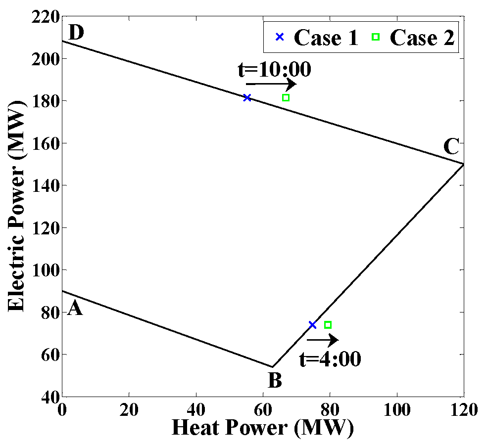
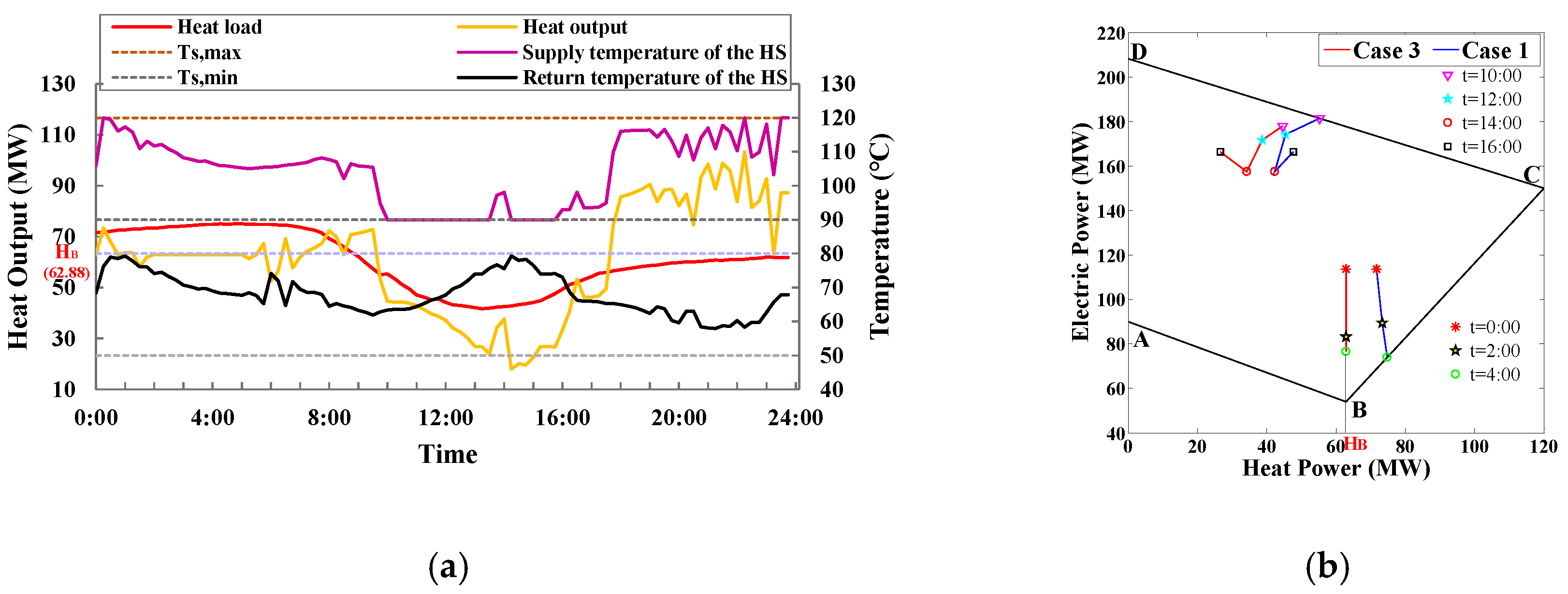
5.1.1. Influence of the Transmission Delay on Flexibility Scheduling

To analyze the impact of the transmission delay in the UHN on flexibility scheduling, the following three scenarios are set for a comparative analysis:
Case 1: Regardless of the dynamic characteristics of the UHN, optimal scheduling is carried out to maximize system flexibility;
Case 2: Considering the dynamic characteristics of the UHN and keeping the supply temperature of the HS in Case 1 unchanged, the flexibility scheduling plan of Case 1 is analyzed;
Case 3: For the model proposed in this paper, the dynamic characteristics of the UHN are considered, and optimal scheduling is performed with the goal of maximizing system flexibility.
Figure 7 shows the supply temperature of the HS for Cases 1 and 2 and the corresponding system flexibility.
According to Figure 7, for the scheduling results of Case 1 (without considering the transmission delay of the UHN), the system flexibility can meet the demand except for the 4:00–5:00 period, with an insufficient downward flexibility rate of 9.8% in the electric load valley period and an insufficient upward flexibility rate of 0% in the electric load peak period. However, in actual operation, due to the transmission delay of the UHN, there will be some deviation between the actual thermal output of the CHP units and the planned thermal output, and there may be a large change in the actual system flexibility, which may even affect the operational safety of the thermal system. For Case 2, the heating system is scheduled based on the optimized supply temperature in Case 1, and it can be observed from its flexibility curve that, in the electric load valley period, the system downward flexibility decreases at 3:00–6:00 and cannot meet the flexibility requirements; during the electric load peak period, the system upward flexibility is reduced and cannot meet the flexibility demand from 10:00 to 11:30. The actual insufficient downward flexibility rate during the electric load valley period is 29.3%, and the actual insufficient upward flexibility rate in the electric load peak period is 2.2%. Overall, these results show that ignoring the delay characteristics of the UHN will cause a significant difference between the actual system flexibility and planned system flexibility and accordingly goes against the penetration of wind power and the sufficient supply of electric load. In particular, the actual values of downward flexibility are negative at 4:00–4:45, indicating that the scheduling plan without considering the transmission delay of the UHN is infeasible.
Moreover, flexibility scheduling that does not consider the transmission delay may also destroy the operational security of the heating system. Figure 8 shows the supply and return node temperatures in Case 1 and Case 2.
According to Figure 8a, the dispatched return temperature of the HS is within the allowable range when the transmission delay of the UHN is not taken into account, and it should be noted that all the node return temperatures are the same in Case 1 because the dynamic characteristics of the UHN are not considered. However, in the actual operation, and due to the transmission delay of the UHN, the return temperatures of HL 1 and HL 3 exceed the lower limit of the return temperature at 0:00–6:30, the return temperature of HL 2 crosses the lower limit at 0:00–8:00 and the return temperature of the HS crosses the lower limit during 3:00–10:00, thus breaking the operational safety of the heat system, as shown in Figure 8b.
The thermal output of the CHP unit changes following the change in the HS return temperature. Figure 9 shows the scheduling results of the CHP unit output in Case 1 and Case 2 at 4:00 and 10:00. According to the supply temperature dispatched in Case 1, the actual thermal output of the CHP unit will exceed its feasible region, which further illustrates that a flexibility scheduling plan that does not consider the dynamic characteristics of the UHN may not be feasible in practice.
Next, we analyzed the results of the flexibility scheduling model proposed in this paper. Figure 10 shows the scheduling results of the proposed model (Case 3) and the scheduling results of Case 1.
Compared with Case 1, the model proposed in this paper reduces the insufficient rate of downward flexibility during the electric load valley period from 9.8% to 0%, and the upward flexibility during the electric load peak period is also improved. Among them, at 0:00–0:45 and 4:30–10:00, the system flexibility of Case 1 and Case 3 is kept at 40 MW, which is the sum of the maximum upward or downward climbing rate of all units within 15 min.
The next section of the research is concerned with the reasons for the improvement in the flexibility of the proposed model, which is analyzed from the temperature dynamic characteristics of the UHN and the power output changes of the CHP units. Figure 11 shows the supply and return temperatures of the HS and operational status of the CHP units.
In Figure 11a, Ts,max and Ts,min are the upper and lower limits of the HS supply temperature, respectively, and HB (62.88 MW) is the thermal power value corresponding to point B in the feasible region of the CHP unit. After considering the dynamic characteristics of the UHN, the thermal output of the CHP units is no longer required to be consistent with the HL at all times, whereas the thermal output of the CHP units is adjusted according to the flexibility requirements at different times, thereby improving system flexibility. According to Figure 11a, in the 0:00–4:00 electric load valley period, by adjusting the supply temperature of the HS, the thermal output of the CHP unit is basically kept near 62.88 MW (HB), where the CHP has the largest downward adjustable electric capacity; during 10:00–16:00 of the peak period, the HS supply temperature is basically maintained at the minimum value to minimize the heat output of the CHP unit and increase the upward adjustable electric capacity.
The results in this section indicate that after considering the actual dynamic characteristics of the UHN, the thermal output of the CHP unit can be adjusted within a certain range by reasonably regulating the supply temperature of the HS. Thus, the proposed model provides a greater margin for power adjustment and provides an adequate flexibility system to cope with RE fluctuations.

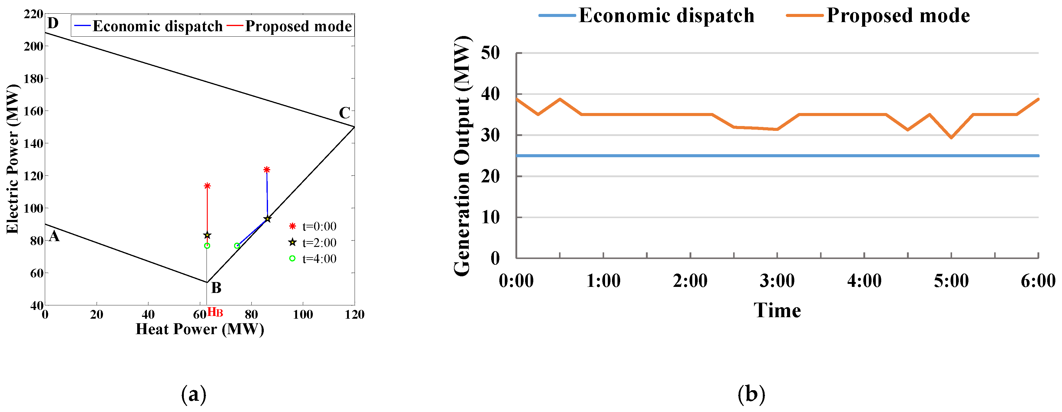
5.1.2. Comparative Analysis of Flexibility Scheduling and Economic Scheduling

Economic dispatch is the main dispatch mode of the UIES. This section will analyze the results of flexibility scheduling and economic scheduling and investigate the applicability of the proposed flexibility scheduling model. Among them, the economic dispatch model takes the minimum operating cost of each unit as the objective function, and the cost coefficients of each unit come from [26]. Figure 12 compares the system downward flexibility of the proposed model and the economic dispatch model during the valley load period and the system upward flexibility during the peak load period.
It can be seen from Figure 12 that according to the economic dispatch model, the insufficient downward flexibility rate of the system during the valley load period is 20.5%, and wind curtailment is required for some periods. Moreover, during the peak load period, the downward flexibility rate of the system is 44.9%, and most of the time, part of the load needs to be removed. It indicates that in this case, the effect of the flexibility scheduling is better than the economic scheduling.
Next, the system flexibility differences between the two scheduling models are analyzed. Figure 13 shows the system flexibility of the proposed model and the economic dispatch model in the valley and peak load periods.
Figure 13 shows that, since CHP units supply both electricity and thermal energy, the power generation cost of CHP units is lower than that of TPP units, and thus CHP power generation will be given priority for the economic dispatch. During the electric load valley period, the electric demand is mainly supplied by the CHP units, which can provide certain downward flexibility, while the TPP units all operate at the minimum output, and there is no downward adjustable capacity. The system cannot meet the flexibility requirements at 1:00–4:00. During the peak load period, the CHP unit basically operates at the upper limit of power generation, having no upward adjustable capacity, while the upward adjustable capacity of TPP units cannot meet the flexibility requirements. In the flexibility dispatch, during the valley load period, the thermal output of the CHP unit is adjusted to HB, which has the largest downward adjustable capacity. At the same time, the TPP units have a certain downward adjustable capacity within their climbing rate limits by reasonably dispatching the electric output of the TPP units; during the peak load period, the thermal output of the CHP unit is reduced to increase its upward adjustable capacity, while at the same time, the TPP units also have a larger upward adjustable capacity. Thus, the proposed model can meet both the flexibility demands in the valley load period and peak load period. Taking the valley load period as an example, Figure 14 shows the unit output status of the economic dispatch model and the proposed flexibility dispatch model.
The effect of flexibility scheduling is related to the prediction error of wind power. When the prediction accuracy of wind power is approximately unchanged, the prediction error is directly related to the level of wind power. The following is the analysis of the comprehensive operating costs of the economic dispatch and flexibility dispatch models under different levels of forecasted wind power. Figure 15 shows the overall cost structure of the two scheduling models when the predicted wind power generation relative to the peak load ratio varies from 5% to 25%. Under different ratios of wind generation, the shapes of the predicted wind power curve and the actual power curve remain unchanged, as shown in Figure 6b.
As shown in Figure 15, under any proportion of predicted wind power, the unit operating cost of the economic dispatch model is less than that of the flexibility dispatch model. However, as the ratio of wind power generation increases, the economic operating model will lead to wind curtailment and load shedding during actual operation. When wind power generation accounts for 10% or more of the maximum electric load, the superiority of the flexibility scheduling model gradually becomes more apparent. In particular, the load-shedding cost will account for 80.9% of the unit operating cost when the percentage of wind power generation reaches 25%. It shows that for the UIES with a high installed capacity of wind generation, when the forecasted wind power is large the next day, the flexibility scheduling model can be used to make the operation plan of each unit to avoid the loss caused by insufficient flexibility.

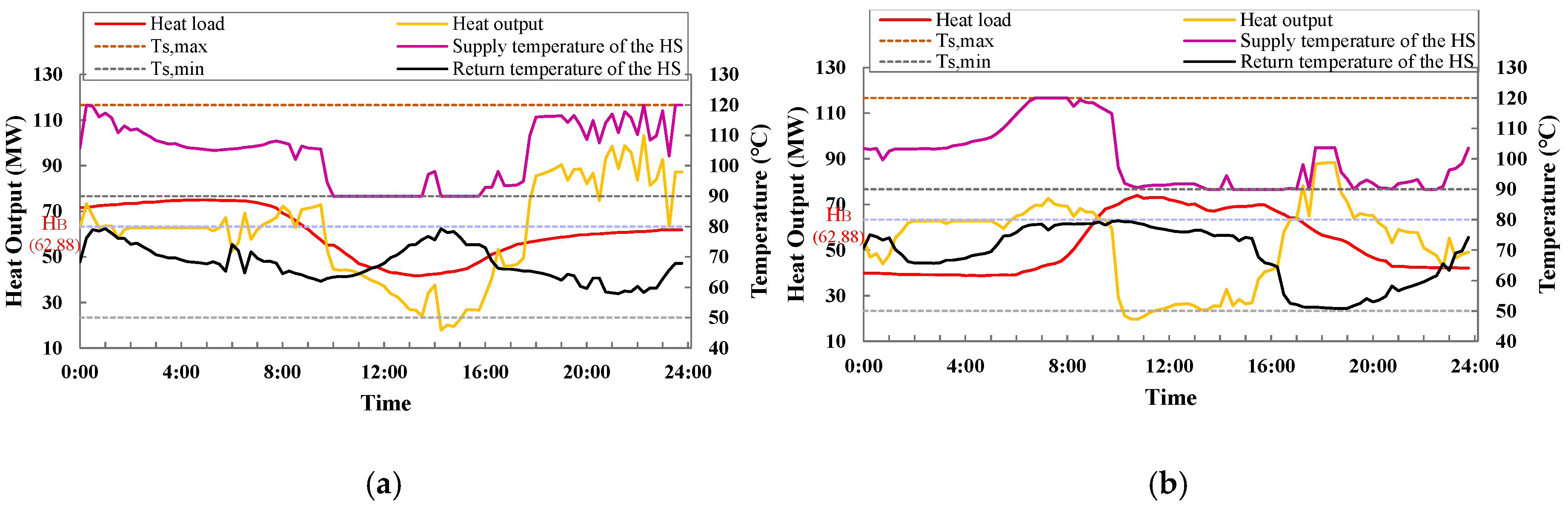
5.1.3. Impact Analysis of the HL Type

To analyze the impact of the type of HL on system flexibility, the HL type in Case 3 is changed from residential user to commercial user, which is set as Case 4 to compare with Case 3. Figure 16 shows the HLs of commercial and residential users, as well as the electric load. It can be seen that the peak and valley periods of the commercial HL are basically consistent with the electric load, which is completely opposite to that of residential users.
Figure 17 compares the system flexibility in Case 3 and Case 4 during the valley and peak load periods.
As can be observed from Figure 17, there is little difference in the level of flexibility between the two scenarios, and the system flexibility demands in each period can be met.
Subsequently, the two cases were analyzed from the change in the node supply and return temperatures. Figure 18 compares the supply and return temperatures at the HS, as well as the heat output between the pre- and post-changing HLs.
Figure 18 shows that there is a certain difference in both the HS supply and return temperature curves between Case 4 and Case 3, whereas there is little change in the temperature difference between the HS supply and return temperatures, resulting in a small change in the thermal output, which makes the change in system flexibility under the two cases small.
Overall, these results indicate that the type of HL has little influence on the system flexibility. The heat output of the CHP unit at different time periods can be adjusted by reasonably optimizing the HS supply temperature for different users, thus meeting the downward and upward flexibility demands of the system.

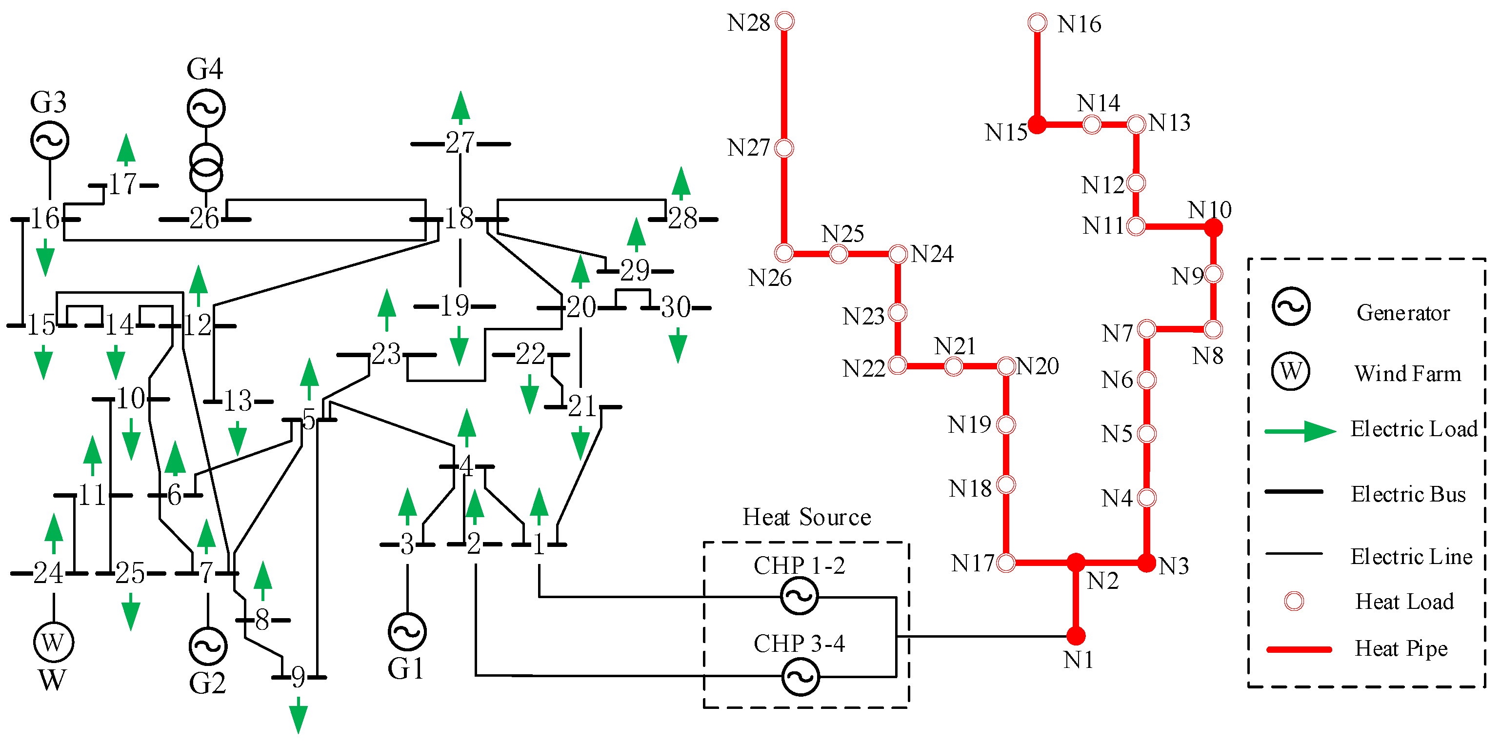
5.2. Practical-Scale System

To further verify the effectiveness of the proposed model, this section uses the heat and power networks of a real city for the simulation verification. The network structure is shown in Appendix B. The heating network parameters come from [30], and the detailed data of the thermoelectric system and unit parameters are provided in Appendix B. The total power capacity of this system is 1.44 GW, including 0.82 GW from CHP units, and 0.3 GW from wind turbines. The trend of electrical and thermal load as well as the wind power is consistent with the small-scale case, where the maximum thermal load is 331 MW, the maximum electrical load is 1073 MW and the maximum predicted wind power is 200 MW.
Figure 19 compares the system flexibility of the proposed model and the economic scheduling model at different periods.
For the proposed model, the insufficient downward flexibility rate during the electric load valley period is 4.32%, and the insufficient upward flexibility rate in the peak load period is 0.60%. For the economic dispatch model, it has an insufficient downward flexibility rate of 4.57% in the valley load period, and the insufficient upward flexibility rate during peak load periods is 47.13%.
Table 1 shows the overall cost composition of the two scheduling models.
According to Table 1, the unit operating cost of the proposed model is USD 601,821, which is USD 40,353 higher than that of the economic dispatch model, but the load-shedding cost is USD 250,790 lower than the economic dispatch model, and the overall cost is 25.78% lower than that of the economic dispatch model.

6. Conclusions

Aiming at a UIHPS with a high percentage of RE, this paper establishes a flexibility scheduling model for a UIHPS considering the dynamic characteristics of the UHN by combining the coupling characteristics of multi-energy system with the dynamic characteristics of a UHN. Through theoretical research and the analysis of case studies, the following conclusions are drawn:
(1)
In the UIES, due to the obvious transmission delay of the UHN, it must be considered in the flexibility scheduling model, otherwise the operational safety of the system may be broken. By making full use of the transmission delay and temperature dynamics of the UHN, the overall flexibility can be improved through the cooperative scheduling of the urban heat and electricity systems, thereby dealing with the random fluctuations of renewable generation effectively;
(2)
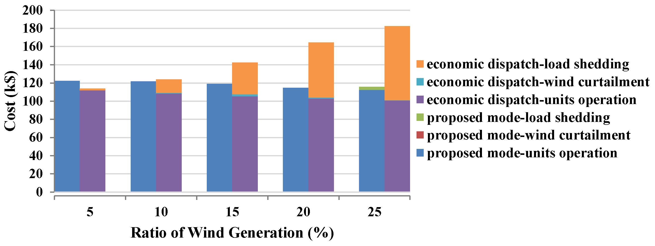
For the UIES with high penetration of RE, when the forecasted renewable generation is relatively large, the flexibility scheduling model can be used to make the operation plan of each unit. Although the unit operating cost is higher than that of the economic dispatching model, the huge cost of load shedding caused by fluctuations of renewable generation can be effectively avoided in the proposed model;
(3)
The type of HL has little effect on the flexibility dispatching results for the UIHPS. For different types of HL, the heat output of the CHP units can be optimized by adjusting the supply temperature of the HS to reduce the impact of different HL peak and valley periods on the system flexibility and effectively meet the flexibility demands of the system.
In the proposed model, we mainly utilize the temperature dynamics of the primary UHN and the coupling characteristics of CHP units to improve the system flexibility. In actual operation, when the prediction accuracy of the HL is rather low, it will cause the actual heat output of CHP units to largely deviate from the planned, and thus affect the system flexibility and RE integration. Furthermore, the thermoelectric coupling characteristics of the substations and the end users also have an effect on the system flexibility. Therefore, we will investigate to improve the forecast accuracy of the HL, and cooperatively consider CHP substations user-side energy equipment to enhance the system flexibility in future research.

Author Contributions

Conceptualization, supervision, writing-review & editing and funding acquisition, W.W.; methodology, software and writing—original draft, Y.S.; writing—review and editing, K.H., H.J. and J.W.; funding acquisition, L.G. and L.W.; resources, C.T. All authors have read and agreed to the published version of the manuscript.

Funding

This research was funded by State Grid Science & Technology Project “Research on simulation analysis model and comprehensive evaluation technology of urban energy internet” (No. 5400-201957186A-0-0-00).

Conflicts of Interest

The authors declare no conflict of interest.

Nomenclature

Abbreviations P g , min t p p / P g , m a x t p p Minimum/maximum electric output of the TPP unit g, MW
UIESUrban integrated energy system R d , g t p p / R u , g t p p Downward/upward ramp rate of the TPP unit g, MW/h
RERenewable energy ρ Density of the hot water, kg/m3
UHNUrban heat network Γ k s Transmission delay of the pipeline k
UIHPSUrban integrated heat and power system D k Diameter of the pipeline k, m
CHPCombined heat and power l k Length of the pipeline k, m
IRREinsufficient ramping resource expectation m ˙ k s Mass flow rate of the supply pipeline k, kg/s
HPHeat pump ψ k Temperature drop coefficient of pipeline k
HSHeat source T a Ambient pipeline temperature, °C
TPPThermal power plant α h Confluence coefficient related to the node h
HLHeat load n j , i Number of paths from node j to node i
CF-VTThe quality regulation mode F j , i v Product of node confluence coefficients in the v-th path from node j to node i
IEAInternational Energy Agency Ψ j , i v Product of pipeline temperature drop coefficients in the v-th path from node j to node i
Indices and sets Γ j , i v Sum of pipeline transmission delays in the v-th path from node j to node i
N S s / N S r Set of HS nodes in the supply/return network m ˙ i L Mass flow rate of HL i, kg/s
N k s / N k e Index of starting and ending nodes of the pipeline k T i , max L s / T i , min L s Maximum/minimum supply temperature of HL i, °C
N j , i v Set of nodes of the v-th path from node j to node i T i , max L r / T i , min L r Maximum/minimum return temperature of HL i, °C
P j , i v Set of pipelines of the v-th path from node j to node i P i j , min / P i j , max Minimum/maximum power of branch ij, MW
N H S Set of HSs U min / U max Minimum/maximum node voltage amplitude of bus i
C H P j Set of CHPs connected to the HS j θ min / θ max Minimum/maximum node voltage phase angle of bus i
P s / P r Set of supply/return pipelinesNgNumber of adjustable generation units
P i u / P i d Set of upstream/downstream pipelines of node iVariables
N s / N r Set of nodes in the supply/return network H g , t c h p / P g , t c h p Heat/electric output of the current operating point of the CHP unit g at time t, MW
N H L Set of HLs α g , t k Combination coefficient corresponding to the k-th corner point in the feasible region of the CHP unit g at time t
T1/T2Index of electric load valley/peak period T j , t S s / T j , t S r Supply/return temperature of the HS j at time t, °C
Parameters P g , t t p p Electric output of the TPP unit g at time t, MW
N K g Number of corner points in the feasible region of the CHP unit g T k , t p s , i n   / T k , t p s , o u t   Inlet/outlet temperature of the pipeline k at time t, °C
H g k / P g k Heat/electric output corresponding to the k-th corner point in the feasible region of the CHP unit g, MW H i , t L Heat load of the heat exchange station i at time t, MW
C g k Cost corresponding to the k-th corner point of the CHP unit g, $ T i , t L s / T i , t L r Supply/return temperature of the HL i at time t, °C
c Specific heat capacity of water, kJ/(kg·°C) T i n , i , t P L / T o u t , i , t P L Inlet/outlet temperature of the equivalent pipe of the heat load i, °C
m ˙ j S Mass flow rate of the HS j, kg/s P i , t t p p / Q i , t t p p Active/reactive power output of TPP units at bus i at time t, MW/Mvar
T j , min S s / T j , max S s Minimum/maximum supply temperature of the HS j, °C P i , t w i n d / Q i , t w i n d Active/reactive power output of the wind farm at bus i at time t, MW/Mvar
T j , min S r / T j , max S r Minimum/maximum return temperature of the HS j, °C P i , t l o a d / Q i , t l o a d Active/reactive power load at bus i at time t, MW/Mvar
R d , g c h p / R u , g c h p Downward/upward ramp rate of the CHP unit g, MW/h f t d / f t u Downward/upward flexibility of UIES at time t, MW
Δ t Dispatch time step, h Δ P t u / Δ P t d Upward/downward fluctuation of wind power at time t, MW
a g , b g , c g Cost coefficients of the TPP unit g Δ f t d / Δ f t u Downward/upward flexibility deficiency rate

Appendix A. Data of Small-Scale Case Study

Table A1. Units parameters.
UnitBusPmax
(MW)
Pmin
(MW)
Qmax
(MW)
Qmin
(MW)
RU
(MW/h)
RD
(MW/h)
a
($/MW2)
b
($/MW)
c
($)
Startup
($)
11301070−4015150.000516.83220.58125
225015200−8025250.001340.62161.87374
36208.254150−12040400.00443.60100600
Table A2. Feasible region and corresponding cost of CHP.
PointHeat Output (MW)Electric Output (MW)Cost ($)
A0902040
B62.88541770
C1201503330
D0208.22910

Appendix B. Data of Practical-Scale Case Study

Figure A1. Schematic diagram of the electricity and heating networks in the practical system.
Energies 13 03273 g0a1
Table A3. Heat network parameters.
idF_nodeT_nodeLength (m)Diameter (m)Conductivity (W/(m·°C))Roughness (m)Flowrate (kg/s)
112100010.120.00051757.012
2232264.510.120.0005596.784
33486510.120.0005596.784
445193910.120.0005489.276
556253110.120.0005397.893
66731510.120.0005320.219
7783000.90.120.0005254.195
8899900.90.120.0005198.075
99106890.90.120.0005150.373
1010112590.90.120.0005150.373
1111122000.80.120.0005109.826
1212133000.80.120.000575.361
1313142600.60.120.000546.066
1414154020.60.120.000521.166
15151616000.350.120.000521.166
16217250010.120.00051160.228
171718250010.120.0005957.334
181819205010.120.0005784.874
191920105010.120.0005638.282
20202118000.90.120.0005513.680
21212217500.90.120.0005407.768
22222326000.90.120.0005317.743
23232419000.90.120.0005241.221
24242524000.80.120.0005176.178
25252619000.80.120.0005120.891
26262728000.60.120.000573.898
27272836000.60.120.000533.953
Table A4. Electric network parameters
F_busT_busr (p.u)x (p.u)b (p.u)F_busT_busr (p.u)x (p.u)b (p.u)
140.00031 0.00180 −0.08495 14150.00267 0.02106 −0.01189
140.00031 0.00180 −0.02242 15160.00051 0.00630 −0.01189
240.00031 0.00180 −0.03879 15160.00051 0.00630 −0.00915
340.00031 0.00180 −0.02000 16170.00024 0.00299 −0.90000
450.00062 0.00367 −0.02130 16170.00024 0.00299 −0.01200
450.00062 0.00367 −0.01000 16180.00710 0.03739 −0.07777
5120.00327 0.01706 −0.01000 16180.00710 0.03739 −0.05500
560.00060 0.00310 −0.09215 19180.00139 0.01094 −0.01204
570.00026 0.00204 −0.04100 19180.00139 0.01094 −0.00862
590.00793 0.04177 −0.10824 20180.00560 0.02948 −0.03318
5230.00499 0.02630 −0.03660 20180.00560 0.02948 −0.04575
890.00292 0.02310 −0.12654 20230.00728 0.03833 −0.00165
780.00131 0.01031 −0.12654 20210.00197 0.01559 −0.20000
670.00011 0.00064 −0.15090 20210.00197 0.01559 −0.20000
670.00011 0.00064 −0.16410 22210.00165 0.00544 −0.15833
6100.00104 0.00543 −0.06128 1210.00148 0.01171 −0.01372
10110.00299 0.01573 −0.00044 1210.00148 0.01171 −0.01372
10110.00299 0.01573 −0.13150 24110.00207 0.00207 −0.43500
10120.00250 0.01315 −0.03596 25110.00207 0.00207 −0.39500
13120.00466 0.01535 −0.57500 26180.00207 0.00207 −0.75000
12150.00400 0.03163 −0.82500 27180.00207 0.00207 −0.75000
12140.00057 0.00452 −0.01696 28180.00207 0.00207 −0.00522
12180.00470 0.02475 −0.03431 29180.00207 0.00207 −0.00695
12180.00470 0.02475 −0.03250 30200.00207 0.00207 −0.01958
Table A5. Units parameters.
UnitBusPmax
(MW)
Pmin
(MW)
Qmax
(MW)
Qmin
(MW)
RU
(MW/h)
RD
(MW/h)
a
($/MW2)
b
($/MW)
c
($)
Startup
($)
1124098300−3001201200.00443.601001700
2124098300−3001201200.00443.601001700
3217060300−3001021020.00443.601001300
4217060300−3001021020.00443.601001300
530.010200−250000.014116.08212.311200
675020200−2525250.014116.08212.311200
7165020700−70025250.052743.66781.521500
82622060999−9991101100.052743.66781.522100
Table A6. Feasible region and corresponding cost of CHPs.
PointCHP 1−2CHP 3−4
Heat Output (MW)Electric Output (MW)Cost ($)Heat Output (MW)Electric Output (MW)Cost ($)
A010027530701927
B10298366250602124
C1351904875701543483
D0240413001702926

References

  1. Alizadeh, M.I.; Moghaddam, M.P.; Amjady, N.; Siano, P.; Sheikh-El-Eslami, M.K. Flexibility in future power systems with high renewable penetration: A review. Renew. Sustain. Energy Rev. 2016, 57, 1186–1193. [Google Scholar] [CrossRef]
  2. Agency, I.E. Empowering Variable Renewables—Options for Flexible Electricity Systems; OECD Publishing: Paris, France, 2009; pp. 13–14. [Google Scholar]
  3. Wu, S.Y.; Wang, P.; Yang, J.; Li, Z.N.; Ouyang, M. Review on interdependency modeling of integrated energy system. In Proceedings of the IEEE Conference on Energy Internet and Energy System Integration, Beijing, China, 26–28 November 2017. [Google Scholar]
  4. Wu, J.; Yan, J.; Jia, H.; Hatziargyriou, N.; Djilali, N.; Sun, H. Integrated energy systems. Appl. Energy 2016, 167, 155–157. [Google Scholar] [CrossRef]
  5. Mancarella, P. MES (multi-energy systems): An overview of concepts and evaluation models. Energy 2014, 65, 1–17. [Google Scholar] [CrossRef]
  6. Niemi, R.; Mikkola, J.; Lund, P.D. Urban energy systems with smart multi-carrier energy networks and renewable energy generation. Renew. Energy 2012, 48, 524–536. [Google Scholar] [CrossRef]
  7. Lannoye, E.; Flynn, D.; O’Malley, M. Evaluation of Power System Flexibility. IEEE Trans. Power Syst. 2012, 27, 922–931. [Google Scholar] [CrossRef]
  8. Zhao, J.Y.; Zheng, T.X.; Litvinov, E. A Unified Framework for Defining and Measuring Flexibility in Power System. IEEE Trans. Power Syst. 2016, 31, 339–347. [Google Scholar] [CrossRef]
  9. Ulbig, A.; Andersson, G. Analyzing operational flexibility of electric power systems. Int. J. Electr. Power Energy Syst. 2015, 72, 155–164. [Google Scholar] [CrossRef]
  10. Marneris, I.G.; Biskas, P.N.; Bakirtzis, E.A. An Integrated Scheduling Approach to Underpin Flexibility in European Power Systems. IEEE Trans. Sustain. Energy 2016, 7, 647–657. [Google Scholar] [CrossRef]
  11. Yang, Y.L.; Wu, K.; Long, H.Y.; Gao, J.C.; Yan, X.; Kato, T.; Suzuoki, Y. Integrated electricity and heating demand-side management for wind power integration in China. Energy 2014, 78, 235–246. [Google Scholar] [CrossRef]
  12. Nuytten, T.; Claessens, B.; Paredis, K.; Van Bael, J.; Six, D. Flexibility of a combined heat and power system with thermal energy storage for district heating. Appl. Energy 2013, 104, 583–591. [Google Scholar] [CrossRef]
  13. Chen, X.Y.; Kang, C.Q.; O’Malley, M.; Xia, Q.; Bai, J.H.; Liu, C.; Sun, R.F.; Wang, W.Z.; Li, H. Increasing the Flexibility of Combined Heat and Power for Wind Power Integration in China: Modeling and Implications. IEEE Trans. Power Syst. 2015, 30, 1848–1857. [Google Scholar] [CrossRef]
  14. Papaefthymiou, G.; Hasche, B.; Nabe, C. Potential of Heat Pumps for Demand Side Management and Wind Power Integration in the German Electricity Market. IEEE Trans. Sustain. Energy 2012, 3, 636–642. [Google Scholar] [CrossRef]
  15. Sayegh, M.A.; Danielewicz, J.; Nannou, T.; Miniewicz, M.; Jadwiszczak, P.; Piekarska, K.; Jouhara, H. Trends of European research and development in district heating technologies. Renew. Sustain. Energy Rev. 2017, 68, 1183–1192. [Google Scholar] [CrossRef] [Green Version]
  16. Sayegh, M.A.; Jadwiszczak, P.; Axcell, B.P.; Niemierka, E.; Brys, K.; Jouhara, H. Heat pump placement, connection and operational modes in european district heating. Energy Build. 2018, 166, 122–144. [Google Scholar] [CrossRef]
  17. Wang, J.D.; Zhou, Z.G.; Zhao, J.N.; Zheng, J.F. Improving wind power integration by a novel short-term dispatch model based on free heat storage and exhaust heat recycling. Energy 2018, 160, 940–953. [Google Scholar] [CrossRef]
  18. Gu, W.; Wang, J.; Lu, S.; Luo, Z.; Wu, C.Y. Optimal operation for integrated energy system considering thermal inertia of district heating network and buildings. Appl. Energy 2017, 199, 234–246. [Google Scholar] [CrossRef]
  19. Salta, M.; Polatidis, H.; Haralambopoulos, D. Industrial combined heat and power (CHP) planning: Development of a methodology and application in Greece. Appl. Energy 2011, 88, 1519–1531. [Google Scholar] [CrossRef]
  20. Lahdelma, R.; Hakonen, H. An efficient linear programming algorithm for combined heat and power production. Eur. J. Oper. Res. 2003, 148, 141–151. [Google Scholar] [CrossRef]
  21. Pirouti, M.; Bagdanavicius, A.; Ekanayake, J.; Wu, J.Z.; Jenkins, N. Energy consumption and economic analyses of a district heating network. Energy 2013, 57, 149–159. [Google Scholar] [CrossRef]
  22. He, P.; Sun, G.; Wang, F.; Wu, H. District Heating Engineering, 4th ed.; China Architecture and Building Press: Beijing, China, 2009; pp. 285–289. [Google Scholar]
  23. Liu, X.Z.; Wu, J.Z.; Jenkins, N.; Bagdanavicius, A. Combined analysis of electricity and heat networks. Appl. Energy 2016, 162, 1238–1250. [Google Scholar] [CrossRef] [Green Version]
  24. Zheng, J.F.; Zhou, Z.G.; Zhao, J.N.; Wang, J.D. Integrated heat and power dispatch truly utilizing thermal inertia of district heating network for wind power integration. Appl. Energy 2018, 211, 865–874. [Google Scholar] [CrossRef]
  25. Yu, D.L.; Tu, C.W.; Wang, Z.L.; Lv, C.; Wang, H.F. Optimal Energy Flow of Combined Electrical and Heating Multi-energy System Considering the Linear Network Constraints. Proc. CSEE 2019, 37, 1933–1944. [Google Scholar]
  26. Li, Z.G.; Wu, W.C.; Wang, J.H.; Zhang, B.M.; Zheng, T.Y. Transmission-Constrained Unit Commitment Considering Combined Electricity and District Heating Networks. IEEE Trans. Power Syst. 2016, 7, 480–492. [Google Scholar] [CrossRef]
  27. Illinois Inst. Technol. Test Data of 6-Bus System for UC-CEHN. Available online: http://motor.ece.iit.edu/data/UCCEHN_6bus.xls (accessed on 14 August 2015).
  28. Song, Z.R.; Shen, F.; Nan, Z.; Zhang, Y.B.; Zhao, L.; Deng, X.Y.; Zhang, N.; Li, H.; Zhang, Z.X.; Ye, W.; et al. Power Grid Planning Based on Differential Abandoned Wind Rate. J. Eng. 2017, 13, 1055–1059. [Google Scholar] [CrossRef]
  29. Awad, A.S.A.; EL-Fouly, T.H.M.; Salama, M.M.A. Optimal ESS Allocation and Load Shedding for Improving Distribution System Reliability. IEEE Trans. Smart Grid 2014, 5, 2339–2349. [Google Scholar] [CrossRef]
  30. Zhou, S.J. Operational Parameters Prediction and Optimization Research of District Heating System Based on Pipe Network Dynamic Model. Ph.D. Thesis, Shandong University, Jinan, China, 2012. [Google Scholar]
Figure 1. Schematic diagram of an urban integrated heat and power system (UIHPS).
Energies 13 03273 g001
Figure 2. Feasible operating region of combined heat and power (CHP).
Energies 13 03273 g002
Figure 3. Schematic diagram of an urban heat network (UHN).
Energies 13 03273 g003
Figure 4. Schematic diagram of the transmission delay.
Energies 13 03273 g004
Figure 5. Modified six-bus power system with a six-node heat system.
Energies 13 03273 g005
Figure 6. Power profiles: (a) electric and heat loads and (b) predicted and actual wind power.
Energies 13 03273 g006
Figure 7. Comparison of system flexibility between Case 1 and Case 2: (a) downward flexibility in the electric load valley period and (b) upward flexibility in the electric load peak period.
Energies 13 03273 g007
Figure 8. Node temperatures: (a) Case 1 and (b) Case 2.
Energies 13 03273 g008
Figure 9. Comparison of the CHP unit heat output in Case 1 and Case 2 at typical times.
Energies 13 03273 g009
Figure 10. Comparison of system flexibility in Case 1 and Case 3: (a) downward flexibility in the electric load valley period and (b) upward flexibility in the electric load peak period.
Energies 13 03273 g010
Figure 11. (a) Dynamic temperature characteristics of the UHN and (b) operational status of the CHP units.
Energies 13 03273 g011
Figure 12. System flexibility in the proposed model and in the economic dispatch model: (a) downward flexibility in the electric load valley period and (b) upward flexibility in the electric load peak period.
Energies 13 03273 g012
Figure 13. Composition of system flexibility in the economic dispatch and proposed models: (a) downward flexibility for the economic dispatch model, (b) downward flexibility for the proposed model, (c) upward flexibility for the economic dispatch model and (d) upward flexibility for the proposed model.
Energies 13 03273 g013
Figure 14. Unit output during the electric load valley period in the economic dispatch and proposed models: (a) electric and heat output of CHP units and (b) electric output of thermal power plant (TPP) units.
Energies 13 03273 g014
Figure 15. Composition of overall cost with different ratios of wind power generation in the proposed and economic dispatch models.
Energies 13 03273 g015
Figure 16. Heat loads in Case 3 and Case 4.
Energies 13 03273 g016
Figure 17. System flexibility in Case 3 and Case 4: (a) downward flexibility in the electric load valley period and (b) upward flexibility in the electric load peak period.
Energies 13 03273 g017
Figure 18. Dynamic temperature characteristics of the UHN and heat output: (a) Case 3 and (b) Case 4.
Energies 13 03273 g018
Figure 19. System flexibility in the proposed and economic dispatch models: (a) downward flexibility in the electric load valley period and (b) upward flexibility in the electric load peak period.
Energies 13 03273 g019
Table 1. Overall cost for different cases.
Cost (k$)Proposed ModelEconomic Dispatch Model
Unit operation601.821563.749
Wind curtailment0.9561.321
Load shedding3.235256.947
Total606.012822.016

