Advanced Control for Hydrogen Pyrolysis Installations ^†

Abstract

Today, hydrogen production plays an important part in the industry due to the increasing use of hydrogen in significant domains, such as chemistry, transportation, or energy. In this paper, we aim to design a numerical control solution based on the thermodynamic analysis of the pyrolysis reactions for hydrogen production and to present novel research developments that highlight industrial applications. Beginning with the evaluation of the technological aspects for the pyrolysis chemical process, the paper studies the thermodynamic evaluation of the system equilibrium for the pyrolysis reactions set, to recommend an appropriate automatic control solution for hydrogen pyrolysis installations. The numerical control architecture is organized on two levels, a control level dedicated to key technological parameters, and a supervisory decision level for optimizing the conversion performances of the pyrolysis process. The data employed for modelling, identification, control, and optimization tasks, were obtained from an experimental platform. The scientific results can be implemented on dedicated equipment, to achieve an optimal exploitation of the industrial pyrolysis process.

1. Introduction

The chemical and petrochemical industry is an area of interest for automatic control, and some of the most representative applications find their place in this domain. The chemical and petrochemical industry has experienced an unparalleled development through the evolution of technological equipment and production lines, as well as through the expansion of production capacity and use of automatic control tools. The pyrolysis installations are plants of high importance in the petrochemical industry. A multi-component set of the pyrolysis reactions is produced mainly by the cracking of hydrocarbons in the presence of steam [1,2,3]. The cracking reactor is the heart of this chemical complex process. For our research interest, hydrogen is the main component in the pyrolysis reactions, being used in significant industries, like chemical, transportation, or energy. Hydrogen production becomes mainstream in the future and the hydrogen energy technology is beginning to penetrate society. Projects of fuel cell vehicles have been carried out many times in Europe, America, and Asia. Fuel cell vehicles were sold, and fuel cell buses also began to run on ordinary roads. The production volume of these fuel cell vehicles will surely grow, and it seems that it will be important to mainstream automobiles in the future [4,5]. For example, more than 100 hydrogen stations have been built in Japan, and it is planned that 160 more will be built in 2020 and about 900 stations will be constructed by 2030 [6,7,8]. Furthermore, the use of hydrogen storage alloy is promoted as an energy stockpile. Hydrogen energy plants using storage alloys have been commercialized in recent years. Hydrogen storage is a technology that enables clean energy on a yearly basis, and it can be regarded as a distinguishing technology. In this way, the development of hydrogen energy technology has made remarkable progress [9,10,11].

The operating and security conditions required by pyrolysis installations for the hydrogen production involves the most recent solutions offered by automatic control tools [12,13]. For this reason, a study of the thermodynamic reactions is needed before proposing a control strategy.

This paper represents the extended version of the authors’ work presented at the 2019 IFAC ACD conference in Bologna, Italy [14]. The newly added contributions are related to the extended evaluation of the state of the art in the domain, which justifies the related novelty and innovation. The interest in hydrogen production in the transportation industry has been justified, and the computing methods for process modelling, identification, control, and supervision were detailed. New simulations were added.

After a short introduction, in Section 2, the paper presents aspects related to the thermodynamic equilibrium analysis of the hydrogen pyrolysis reactions set and to the reproduction possibility of the results obtained on industrial scale. Section 3 proposes the appropriate control systems, designed for key parameters of the pyrolysis reactor. In Section 4, the supervisory system is designed, with the aim to optimize the pyrolysis reactor operating point. Finally, conclusions are given in Section 5.

2. Thermodynamics of the Pyrolysis Chemical Process

The system of pyrolysis reactions is oriented towards obtaining hydrogen at the thermodynamic equilibrium, when the maximum quantity of hydrogen is obtained. The composition of the reaction products is determined at the thermodynamic equilibrium using a numerical procedure. Ethane and water (vapors) are used as raw materials (reagents). Under constant temperature T and pressure P conditions, the system with simultaneous reactions involving a number N of components is characterized by the thermodynamic function—the enthalpy, from Relation (1) [1,2,3]:

$$G=n^T\mu ={\displaystyle \sum }_{i=1}^N{n}_i{\mu }_i$$

(1)

where n is a vector with $n_i$ the number of moles corresponding to each component; i and $\mu$ are the vector of the chemical potentials of each component involved in the reaction.

At thermodynamic equilibrium, the enthalpy of the reaction has the minimum value and respects the conservation of the atomic mass constraints (number of atoms).

$${\displaystyle \sum }_{i=1}^N{a}_{ji}{n}_i=b_j,j=1,2,\dots ,m$$

(2)

where $a_{ji}$ are the elements of the atomic matrix representing the number of atoms of the element j in component i of the system; $b_j$ is the atomic abundance of the chemical element j in the system (number of atoms of element j originally introduced into the system); and m is the number of chemical elements in the reaction system.

For the equilibrium condition, the problem of nonlinear optimization with equality restrictions is formulated as:

$$\begin{gathered} \min \left\{G={\displaystyle \sum }_{i=1}^N{n}_i{\mu }_i\right\} \\ {\displaystyle \sum }_{i=1}^N{a}_{ji}{n}_i=b_j,\hspace{1em}j=1,2,\dots ,m,\hspace{1em}{n}_i\ge 0 \end{gathered}$$

(3)

The system of pyrolysis reactions is described by enthalpy G, given by the following representation:

$$G={\displaystyle \sum }_{i=1}^N{n}_i\left[{\mu }_i^0\left(T\right)+RT\mathit{ln}p+RT\mathit{ln}\frac{n_i}{{{\displaystyle \sum }}_{i=1}^N{n}_i}\right]$$

(4)

where ${\mu }_i^0\left(T\right)$ is the standard chemical potential of component i, and R is the ideal gas constant.

We consider the reaction system to obtain hydrogen as main product, in the following conditions:

-

reaction temperature: $T=1100°K$;

-

pression: $P=3.8 atm$;

-

ratio $\frac{\mathrm{no}.{\mathrm{of} \mathrm{moles} \mathrm{H}}_2\mathrm{O}}{\mathrm{no}.{\mathrm{of} \mathrm{moles} \mathrm{C}}_2{\mathrm{H}}_6}=4/1=r$;

-

reaction products: H₂, CO, CO₂, CH₄, C₂H₂, O₂, H₂O, C₂H₄, C₂H₆ (N = 9);

-

the atomic matrix in

Table 1. Atomic matrix for the product.

Element j	Component i	(1) CH4	(2) C2H4	(3) C2H2	(4) CO2	(5) H2	(6) CO	(7) O2	(8) H2O	(9) C2H6
1	C	0	1	1	1	1	2	2	0	2
2	H	2	0	0	4	4	2	0	2	6
3	O	0	1	1	0	0	0	2	1	0

;

-

the values of the standard chemical potentials in

Table 2. Standard chemical potentials.

Component	CH4	C2H4	C2H2	CO2	H2	CO	O2	H2O	C2H6
Chemical potential	3.42	13.743	17.7	−42.9	0	−22.8	0	−20.1	14.46

;

-

vector of atomic abundance: $b=\left(2;14;4\right)$.

The optimization problem for thermodynamic analysis in (3) is reformulated as follows:

$$\begin{gathered} \min I\left(x\right) \\ {h}_i\left(x\right)=0,\hspace{1em}i=1,2,\dots ,m \\ {g}_j\left(x\right)\ge 0,\hspace{1em}j=m+1,m+2,\dots ,p \end{gathered}$$

(5)

where $I=\frac{G}{RT}$ is the criterion function, x is the vector of component concentrations ($x=n$), h and g express the constraint functions from (3).

In order to solve the problem (5), a nonlinear programming method is proposed through penalty techniques [15,16], which will compute the optimal solution x*. The penalty technique turns (5) into the equivalent problem:

$$\begin{gathered} \underset{x\in C_{adm}}{min}I\left(x\right) \\ {F}^{\left(k\right)}-C(x^{\left(k\right)})\ge 0 \end{gathered}$$

(6)

where $F^{\left(k\right)}$ is the flexible tolerance function calculated at step k; $D(x^{\left(k\right)})$ is the restriction violation (penalty) function.

In the minimization algorithm, $F^{\left(k\right)}$ is decreasing positively:

$$F^{\left(k\right)}\le F^{\left(k-1\right)}\le \dots \le F^{\left(0\right)}$$

(7)

The penalty criterion $C\left(x\right)$ is defined as follows, using its quadratic form:

$$C^2(x)={{\displaystyle \sum }}_{i=1}^m{h}_i^2\left(x\right)+{{\displaystyle \sum }}_{i=m+1}^p{\delta }_i{g}_i^2\left(x\right)$$

(8)

with ${\delta }_i$ the Heaviside operator:

$${\delta }_i=\left\{\begin{array}{ll}0,& g_i\left(x\right)\ge 0\\ 1,& g_i\left(x\right)<0\end{array}\right.$$

(9)

and the admissible domain $C_{adm}$ given by:

$$C_{adm}=\left\{x | h_i\left(x\right)=0,i=1,2,\dots ,m; g_i\left(x\right)\ge 0,i=m+1,\dots ,p\right\}$$

(10)

This penalty technique works based on the concept of quasi-admissibility, defined as:

$$F^{\left(k\right)}\ge C(x^{\left(k\right)})\ge 0$$

(11)

or,

$$F^{\left(k\right)}-C(x^{\left(k\right)})\ge 0$$

(12)

For the case where the intermediate search point $x\left(k\right)$ is not admissible (the inequalities from Relation (5) are not respected), the algorithm proceeds to minimize $C\left(x\right)$ until (12) is met, and then the criterion function $I\left(x\right)$ will be minimized respecting $C_{adm}$.

The algorithm is working to minimize the penalty function $C\left(x\right)$ and to reduce the tolerance function $F^{\left(k\right)}$ in the search process for the solution x*, ensuring corresponding values, such that $C\left(x\right)$ respects (12).

The minimization for criterion functions $I\left(x\right)$ and $C\left(x\right)$ is performed with the evolutionary direct search algorithm BOX, recommended for solving the problems formulated in (6). The BOX method described in [15,16], constructs a COMPLEX geometric figure in the n-dimensional space, which moves in a controlled sequence towards the solution x*, by reflection, expansion, or contraction operations.

The flexible tolerance function $F^{\left(k\right)}$ is calculated at each search level as follows:

$$F^{\left(k\right)}=\min \left\{F^{\left(k-1\right)},\frac{m+1}{n-m+1}{\displaystyle \sum }_{i=1}^{n-m+1}\Vert x_i^{\left(k\right)}-x_C^{\left(k\right)}\Vert \right\}$$

(13)

where m is the number of equality restrictions, $x_i^{\left(k\right)}$ are the peaks of the geometrical search figure at level k, $x_C^{\left(k\right)}$ is the centroid of this geometrical search figure, $F^{\left(k-1\right)}$ is the value of the tolerance criterion at level k-1. The initialization is done by choosing:

$$F^{\left(0\right)}=2\left(m+1\right)a$$

(14)

where a is the side of the initial geometrical search figure.

Considering the pyrolysis reaction simulation at the parameters: $T=1100 K$, $P=3.8 atm$, $\frac{H_{2}O}{C_2{H}_6}=4:1$, the results from

Table 3. Element concentrations for the pyrolysis reaction mixture.

Mixture Elements	CH4	C2H4	C2H2	CO2	H2	CO	O2	H2O	C2H6
Concentration [%]	3.410	0.1451	0.001225	1.094	49.72	18.86	0.2577	26.313	0.0987

, with the hydrogen concentration at thermodynamic equilibrium, were obtained.

Based on the results of this thermodynamic analysis for the pyrolysis process, a control solution for the cracking reactor to the industrial plant is proposed.

3. Nominal Control Level Design

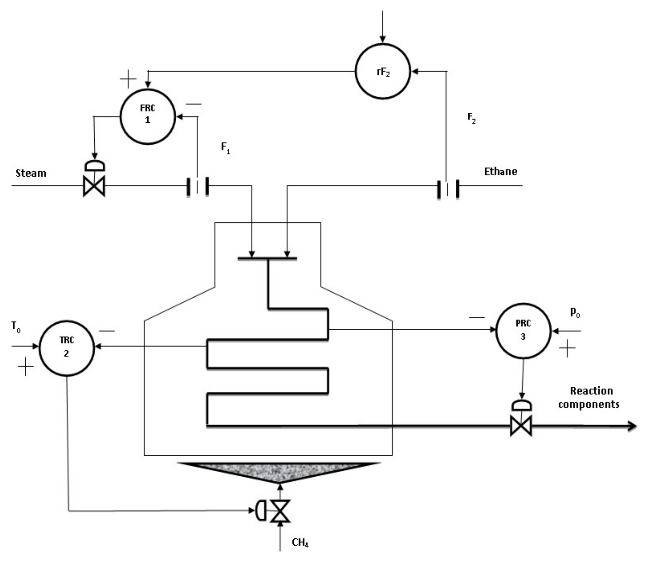
By taking the results of the thermodynamic reaction analysis from Section 2 into account, a control solution for the pyrolysis reactor was proposed, in order to handle two major aspects concerning the operation of the chemical process: to maintain a good ratio between the quantities of reactants, steam and ethane, that are given to the installation, in a proportion 4:1, and to ensure the reaction conditions regarding the temperature and the pressure inside the reactor. Furthermore, we have considered a control structure which involves three closed loops, presented in Figure 1: FRC-1, control loop for steam/ethane flow ratio; TRC-2, control loop for temperature; PRC-3 control loop for pressure.

For the control solution, RST polynomial control was recommended to assure the construction of the two-level proposed architecture, offering independent performances in tracking and control [12,17,18,19].

The design of the polynomials $R(z^{-1})$, $S(z^{-1})$ and $T(z^{-1})$ is performed in two steps. The closed-loop poles are defined by the desired characteristic polynomial, $P(z^{-1})$, as regulation objective, and $R(z^{-1})$ and $S(z^{-1})$ polynomials are computed by the Diophantine equation:

$$P\left(z^{-1}\right)=\widehat{A}\left(z^{-1}\right)S\left(z^{-1}\right)+\widehat{B}\left(z^{-1}\right)R\left(z^{-1}\right)$$

(15)

where the polynomials $\widehat{A}\left(z^{-1}\right)$ and $\widehat{B}\left(z^{-1}\right)$ represent the discrete model of the process.

The Equation (15) has a single unique solution for:

$$\begin{gathered} rank\left(\widehat{A}\left(z^{-1}\right)\right)=na \\ rank\left(\widehat{B}\left(z^{-1}\right)\right)=nb \\ rank\left(P\left(z^{-1}\right)\right)=np\le na+nb-1 \\ rank\left(S\left(z^{-1}\right)\right)=ns=nb-1 \\ rank\left(R\left(z^{-1}\right)\right)=nr=na-1 \end{gathered}$$

(16)

The polynomial Equation (15) can be solved by means of the linear algebraic system:

$$Mx=p$$

(17)

where $M$ is the Sylvester matrix of dimensions $\left(na+ns\right)\times \left(na+ns\right)$ and

$$\left[\begin{array}{c}{x}^T\triangleq \left[1 s_1 s_2\dots s_{ns}, r_0 r_1 \dots r_{na+ns-1}\right]\\ p^T\triangleq \left[1 p_1 p_2 \dots p_{na+ns-1}\right]\end{array}\right.$$

(18)

where $p_i$ are the coefficients of the characteristic polynomial $P(z^{-1})$, $s_i$ and $r_i$ are the coefficients of the $S(z^{-1})$ and $R(z^{-1})$ unknown polynomials, respectively. The solution of the algebraic Equation (17) is obtained by the inversion of the matrix $M$:

$$x=M^{-1}p$$

(19)

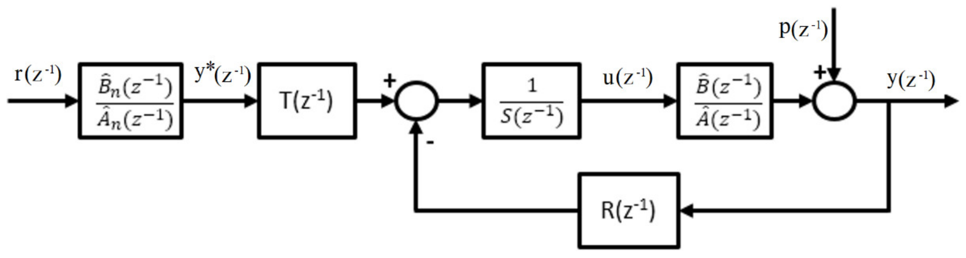
The polynomial $T(z^{-1})$ is determined in order to find the reference trajectory $y^{*}\left(z^{-1}\right)$, the output of the trajectory generator, given by the pair (${\widehat{A}}_n\left(z^{-1}\right),{\widehat{B}}_n\left(z^{-1}\right)$), and to assure the output of the global control system to reference trajectory, $y\left(z^{-1}\right)=y^{*}\left(z^{-1}\right)$ (see Figure 2).

3.1. Control of Stream/Ethane Flow Ratio

The first loop ensures the control of the steam flow to the hydrogen reactor, respecting the imposed ratio. Since steam flow respects the ratio imposed with ethane flow, it is thus achieved the control of both parameters. In order to determine the control algorithm for the steam flow which is pumped into the reactor, we have analytically determined the mathematical model based on the flow equations provided by the parameters of the technological pipe, from the experimental platform [18,19].

Let us consider the pipe with $Q$—flow rate, $\Delta P$—differential pressure across the pipe, $\alpha$—flow coefficient, $S$—pipe section, and $\rho$—fluid density. Considering the short pipe is equivalent to a hydraulic resistance for which the following relation is valid:

$$Q^2={\alpha }^2 S^2\frac{2\Delta P}{\rho }$$

(20)

Using the technological values for the steam flow process, after some calculus operations (linearization and normalization), we will arrive to the non-dimensional linearized model.

For the fluid flow in stationary state, the forces acting on the system are in equilibrium:

$$\Delta P_{0}S-\frac{Q_0^2\rho }{2{\alpha }^2{S}^2}S=0$$

(21)

where $\Delta P_{0}S$ is the active force of pressure on the liquid and $\frac{Q_0^2\rho }{2{\alpha }^2{S}^2}S$ is the reactive force due to the restriction.

In the dynamic state, the difference between both forces is compensated by the inertial force (time variation of quantity of movement):

$$\Delta P\left(t\right)S-\frac{Q^2\left(t\right)\rho }{2{\alpha }^2{S}^2}S=\frac{d}{dt}\left(M\nu \right)$$

(22)

where $M$ represents the mass of the fluid in the pipe and $\nu$ is its velocity. Therefore, we have:

$$\Delta P\left(t\right)S-\frac{Q^2\left(t\right)\rho }{2{\alpha }^2{S}^2}S=\rho L\frac{dQ\left(t\right)}{dt}$$

(23)

In general, we work in stationary state and we consider small variations around an operating point, which translates into:

$$\Delta P\left(t\right)=\Delta P_0+\Delta \left(\Delta P\left(t\right)\right)=\Delta P_0+\Delta p\left(t\right)$$

(24)

$$Q\left(t\right)=Q_0+\Delta Q\left(t\right)$$

(25)

From Equation (23) and Relations (24) and (25), we get:

$$[\Delta P_0+\Delta p\left(t\right)]S-\frac{{[Q_0+\Delta Q\left(t\right)]}^2\rho }{2{\alpha }^2{S}^2}S=\rho L\frac{d\left[Q_0+\Delta Q\left(t\right)\right]}{dt}$$

(26)

By extracting the stationary regime expressed by (26), we get:

$$\Delta p\left(t\right)S-\frac{2\rho Q_0\Delta Q\left(t\right)+\rho \Delta Q{\left(t\right)}^2}{2{\alpha }^2{S}^2}S=\rho L\frac{d\left[\Delta Q\left(t\right)\right]}{dt}$$

(27)

In this equation, which corresponds to the non-linear knowledge model, $\Delta p\left(t\right)$ represents the variation $\Delta \left(\Delta P\left(t\right)\right)$ of the differential pressure.

By ignoring the quadratic term $\Delta Q^2\left(t\right)$ in Equation (27), and using the normalized values for $Q\left(t\right)$ and $p\left(t\right)$ with respect to stationary state, with the notations:

$$\begin{array}{c}y\left(t\right)=\frac{\Delta Q\left(t\right)}{Q_0}\\ u\left(t\right)=\frac{\Delta p\left(t\right)}{\Delta P_0}\end{array}$$

(28)

the final model becomes:

$${\alpha }^2\frac{V_0}{F_0}\frac{dy\left(t\right)}{dt}+y\left(t\right)=\frac{1}{2} u\left(t\right)$$

(29)

By including the actuator and the flow sensor [12,20] for a sampling period of 0.5 s, the discrete dynamic model of the steam flow process has been obtained:

$$H_{P1}\left(z^{-1}\right)=\frac{0.03964z^{-1}+0.006944z^{-2}}{1-0.8484z^{-1}+0.001634z^{-2}}$$

(30)

Taking into consideration this model, the controller was designed to ensure the desired performance using the RST polynomial control algorithm, represented in Figure 2.

The control polynomials R, S and T were computed using the poles allocation method [20]. For the ratio control system, we have obtained the control polynomials in (31):

$$\begin{array}{l}{R}_1\left(z^{-1}\right)=6.254-5.126z^{-1}+0.01z^{-2}\\ S_1\left(z^{-1}\right)=1-0.956 z^{-1}-0.043 z^{-2}\\ T_1\left(z^{-1}\right)=21.466-33.426z^{-1}+13.098z^{-2}\end{array}$$

(31)

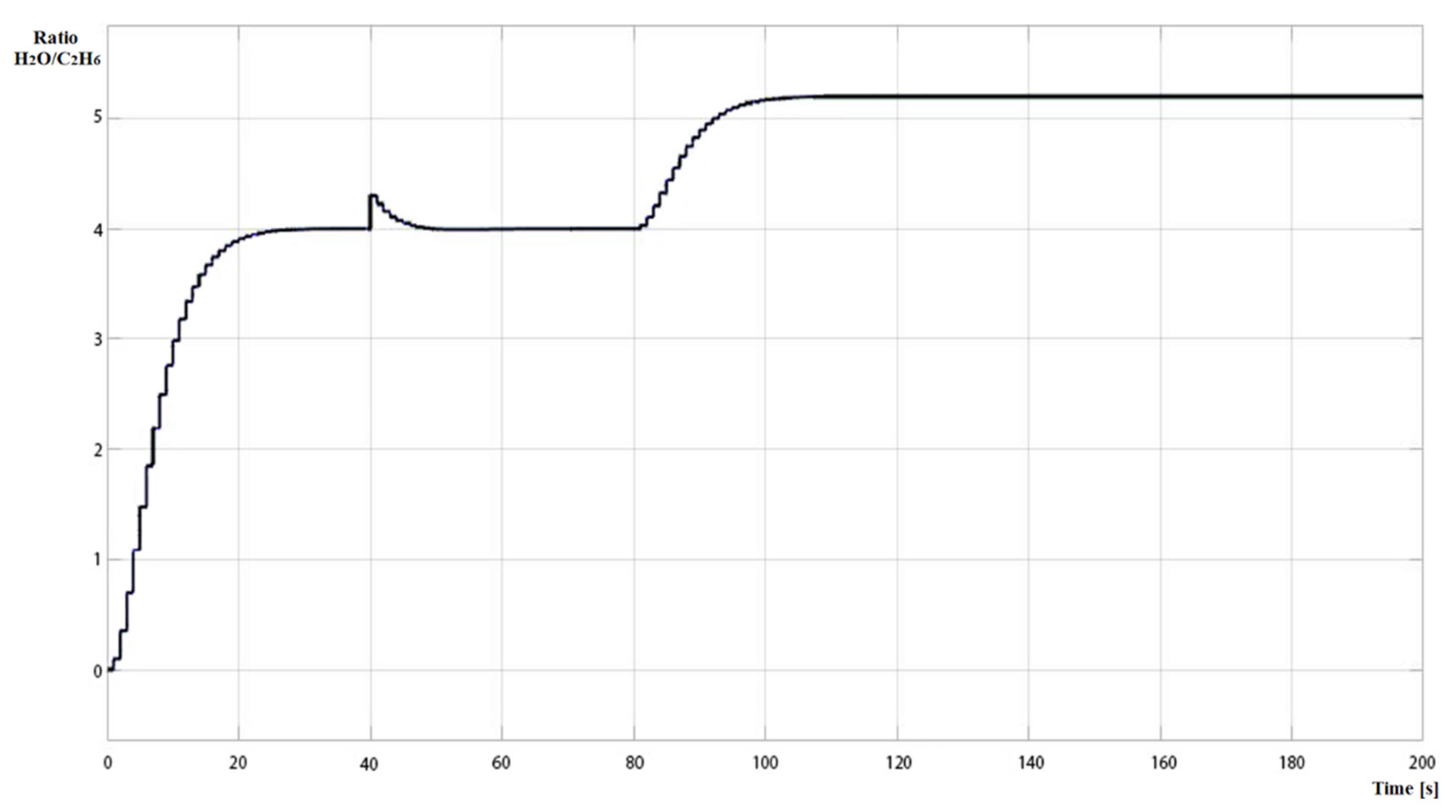
To validate the performances in closed loop, the Matlab/Simulink simulation environment was used. The results of the simulation are shown in Figure 3. It can be noticed that the RST controller ensures in closed loop both tracking and regulation performances for the steam/ethane ratio system [12,21].

3.2. Control of Reaction Parameters

It is of utmost importance that the values of the temperature and the pressure are maintained within the boundaries of the admissible operating domain so that the process functions properly and the reactor walls are not submitted to any risk of degradation. In this case, the temperature within the median section of the reactor is controlled by the CH₄ combustion flow that heats the reactor [22]. The automatic control solution should be able to provide the possibility of maintaining the temperature value in the $(1100–1150 K)$ interval and the pressure value, in the interval $(3.7–4.4 atm)$. By controlling the temperature and the pressure inside the reactor, the reaction equilibrium state is ensured.

In this case, the proposed solution must attain two tasks: the data acquisition and identification of the dynamic models from the experimental pyrolysis platform and, respectively, the control system design of the major parameters of the process. The physical data acquired from the plant are used for the identification of the mathematical models. After the identification process was completed, by using the Least Squares Recursive Experimental Method (LSREM), the models were validated using the whiteness test [12]. A dedicated software for experimental identification, WINPIM [20], was used.

The model identified and validated for the reactor temperature is:

$$H_{P2}\left(z^{-1}\right)=\frac{0.0471z^{-1}}{1-1.614z^{-1}+0.6534z^{-2}}$$

(32)

Moreover, the model identified and validated for the reactor pressure is:

$$H_{P3}\left(z^{-1}\right)=\frac{0.00598z^{-1}}{1-1.68365z^{-1}+0.7073z^{-2}}$$

(33)

The controllers were designed to ensure the desired tracking and regulation performances, using RST polynomial control algorithms. The discrete control polynomials R, S, T were computed by poles allocation methods using a model-based control design software WINREG [20].

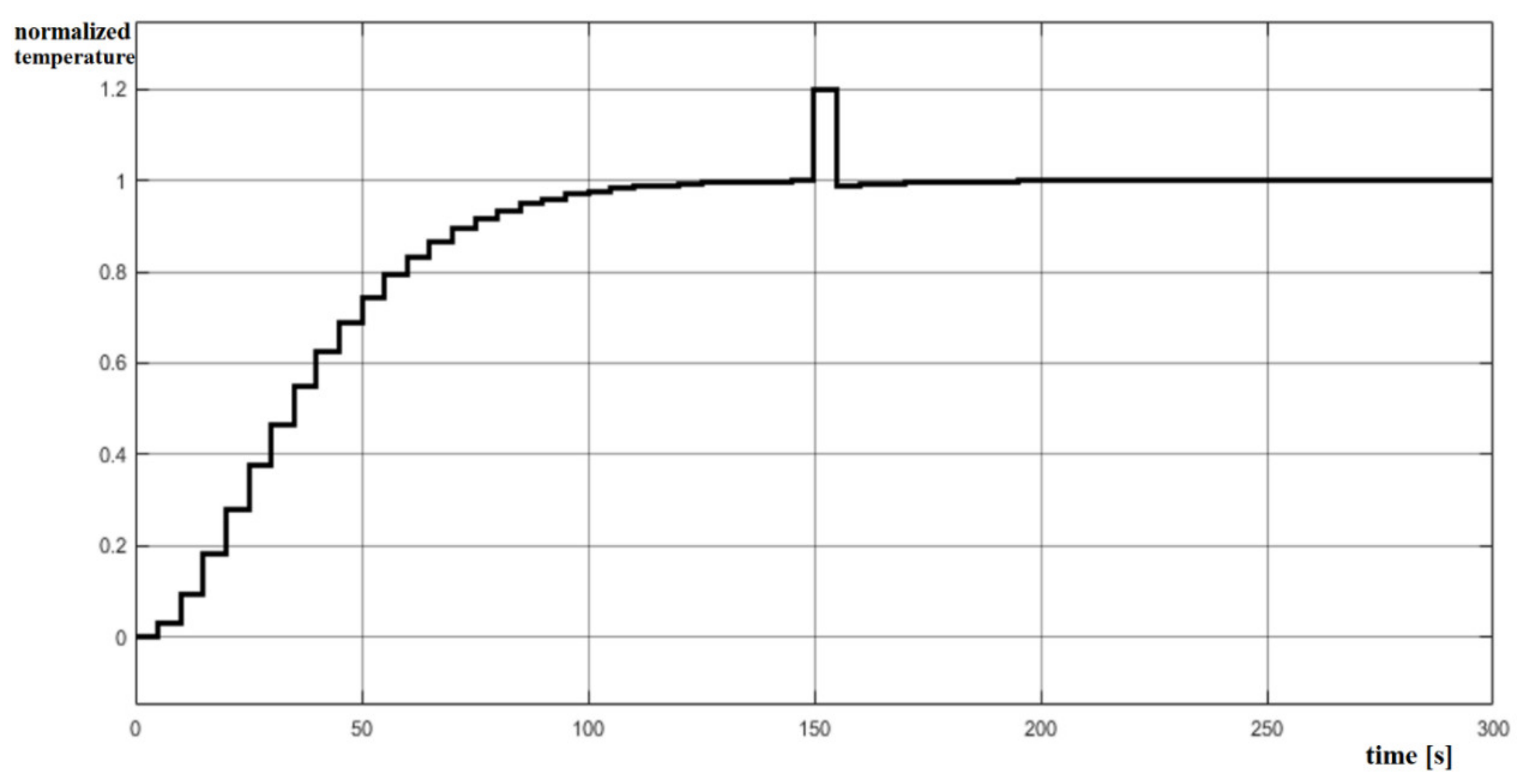
For the temperature control system, we have obtained the control polynomials in (34):

$$\begin{array}{l}{R}_2\left(z^{-1}\right)=22.277-35.061z^{-1}+13.872z^{-2}\\ S_2\left(z^{-1}\right)=1-z^{-1}\\ T_2\left(z^{-1}\right)=21.231-33.222z^{-1}+13.079z^{-2}\end{array}$$

(34)

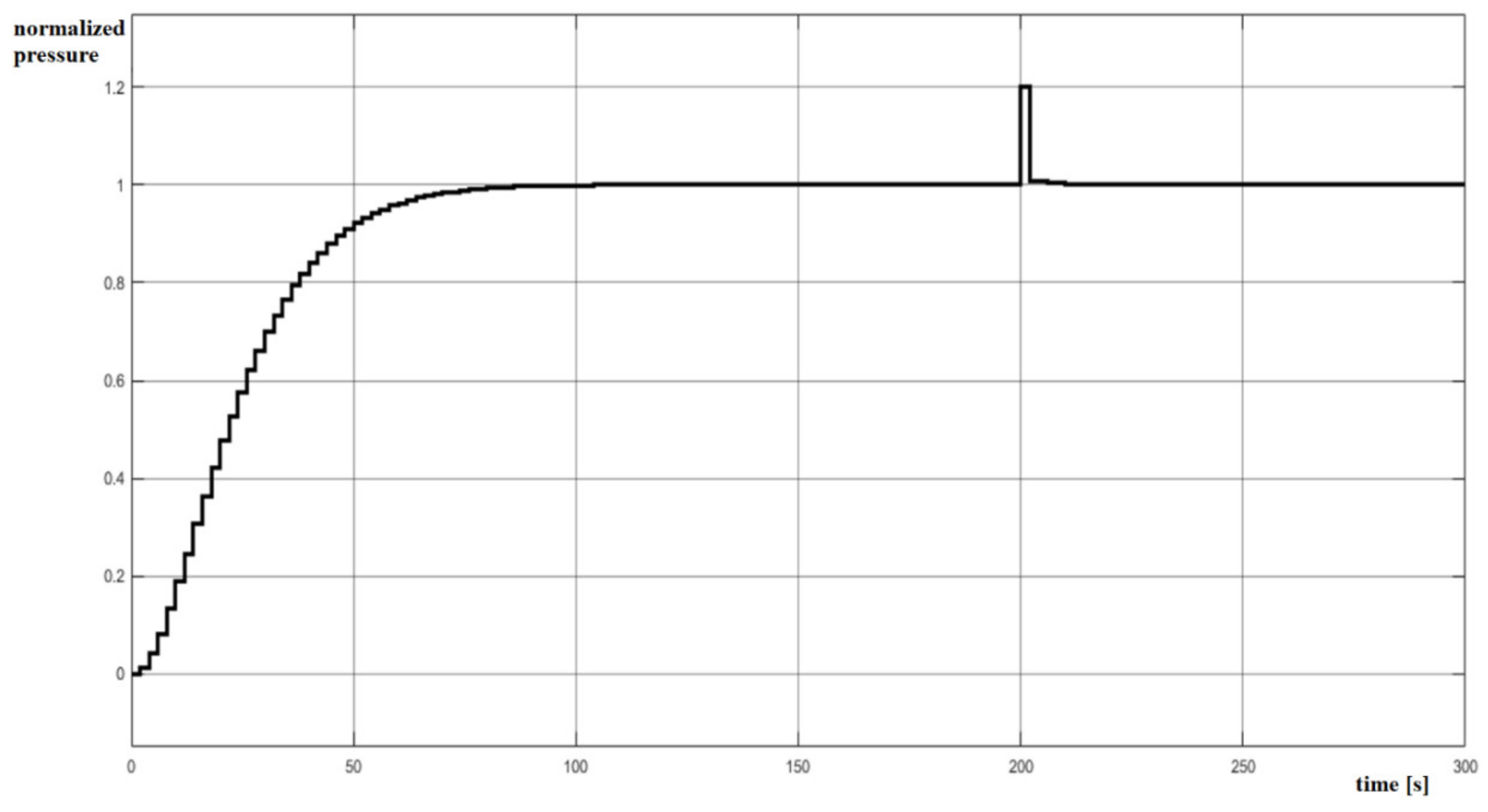
Figure 4 shows the dynamic response of the closed loop temperature control system when a 20% step disturbance is added.

For the pressure control system, we have obtained the control polynomials in (35):

$$\begin{array}{l}{R}_3\left(z^{-1}\right)=160.732-275.495z^{-1}+118.277z^{-2}\\ S_3\left(z^{-1}\right)=1-z^{-1}\\ T_3\left(z^{-1}\right)=167.224-288.039z^{-1}+124.329z^{-2}\end{array}$$

(35)

Similarly, Figure 5 shows the response of the closed loop pressure control system when a 20% step disturbance is added.

For all three systems (FRC-1, TRC-2, PRC-3), the R, S polynomials were computed solving the polynomial Diophantine equation and the T polynomial was computed by assuring the tracking performances for the closed loop systems [18,19].

The RST controllers ensure that the desired tracking and regulation performances for the closed loop systems are met.

3.3. Robust Control Solution

The main goal is to design the robust control systems for temperature and pressure that can provide a way of preserving the performances obtained in simulation on the physical pyrolysis reactor in the presence of disturbances (ethane quality) or modeling uncertainties [18,19,20].

The robustness design is based on the disturbance-output sensitivity function of closed loop system. The sensitivity function for the polynomial RST systems (computed) defined as:

$$S_{py}\left(z^{-1}\right)=\frac{\hat{A}\left(z^{-1}\right)S\left(z^{-1}\right) }{\hat{A}\left(z^{-1}\right)S\left(z^{-1}\right)+\hat{B}\left(z^{-1}\right)R\left(z^{-1}\right)}$$

(36)

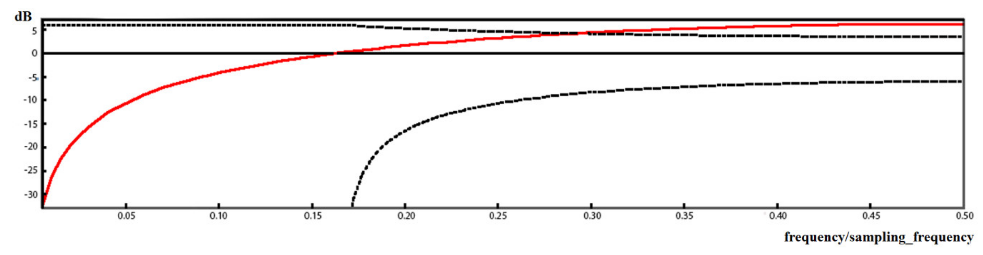
where $\hat{A}\left(z^{-1}\right)$ and $\hat{B}\left(z^{-1}\right)$ are the two polynomials of the identified process model, and $R\left(z^{-1}\right)$ and $S\left(z^{-1}\right)$ are the control polynomials computed earlier. It is desirable for the maximum value of the output sensitivity function to be as low as possible.

For each robust control system, we imposed a usually maximum of 6 dB for the output sensitivity function.

The sensitivity function of the previously designed nominal temperature control system does not meet this requirement, as shown in Figure 6.

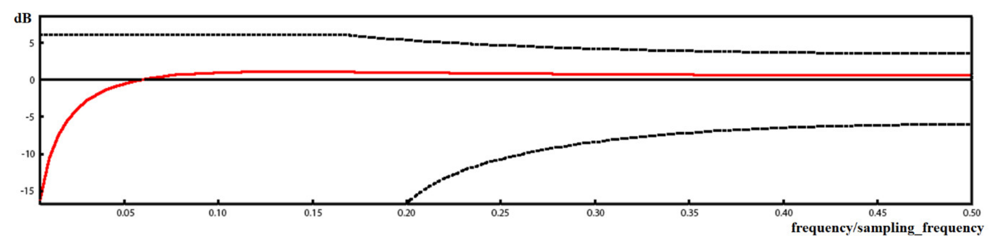
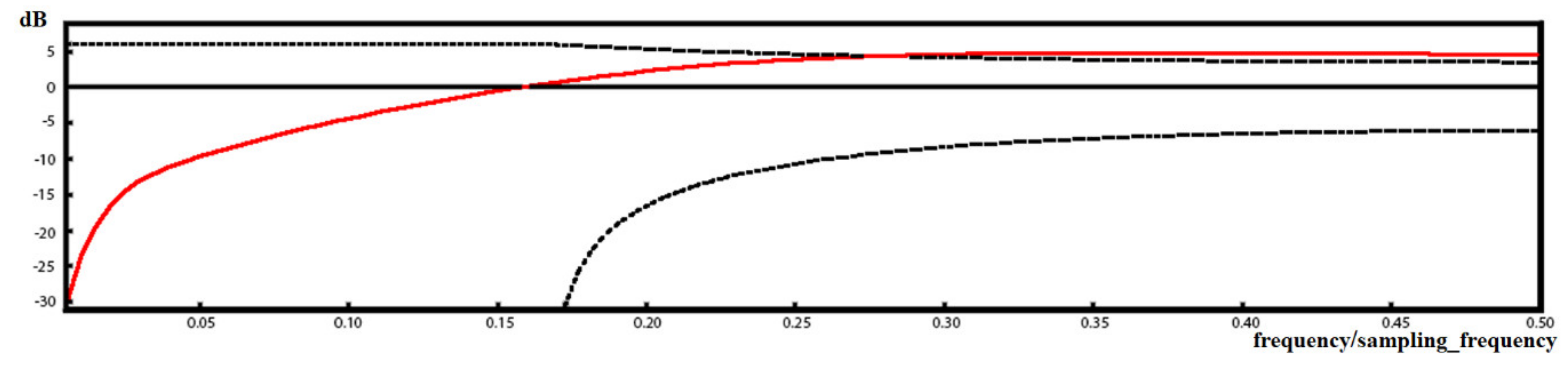
To improve the controller, a pair of complex auxiliary poles was added to the characteristic polynomial, given by the denominator of the sensitivity function. The new robust control polynomials are:

$$\begin{array}{l}{R}_2\left(z^{-1}\right)=3.42-5.53z^{-1}+2.24z^{-2}\\ S_2\left(z^{-1}\right)=1-1.24 z^{-1}+0.24z^{-2}\\ T_2\left(z^{-1}\right)=21.22-60.68z^{-1}+65.15z^{-2}-31.19z^{-3}+5.63z^{-4}\end{array}$$

(37)

The sensitivity function of the new closed loop system meets the imposed 6 dB limit (1.7 dB), which makes the new controller a robust one, see Figure 7.

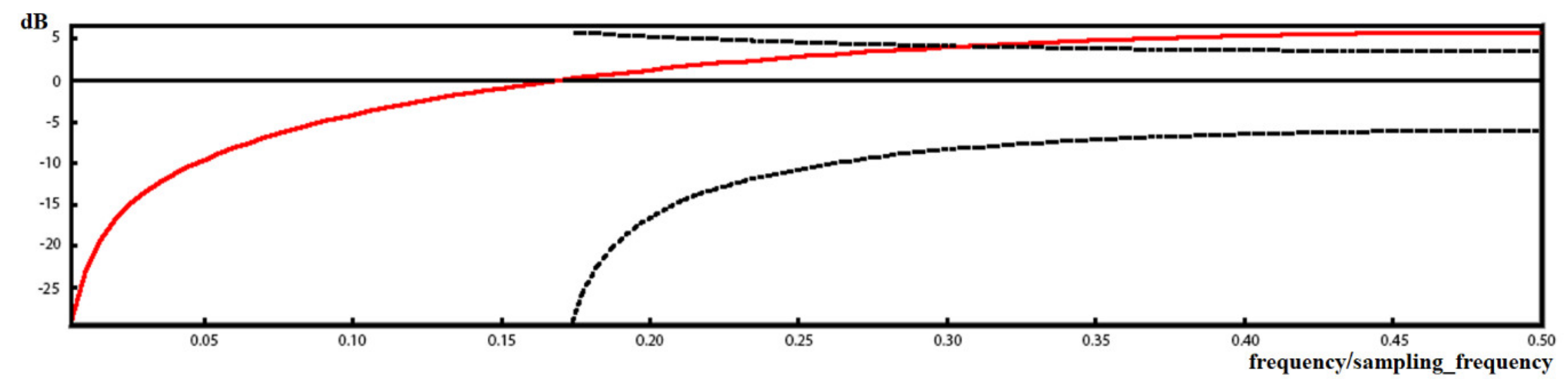
For the pressure control system, we have used a similar approach, since we encountered a similar situation, see Figure 8.

We added the robust correction, by adding a pair of real stable poles to the characteristic polynomial, and obtained the following control polynomials:

$$\begin{array}{l}{R}_3\left(z^{-1}\right)=152.833-267.49z^{-1}+118.277z^{-2}\\ S_3\left(z^{-1}\right)=1-1.15 z^{-1}+0.15z^{-2}\\ T_3\left(z^{-1}\right)=167.224-295.938z^{-1}+132.335z^{-2}\end{array}$$

(38)

The new controller is a robust one, as illustrated in Figure 9.

To summarize, the two control systems achieve the desired robustness margin while preserving the nominal performances.

4. Supervisory Level Design

The optimal operating point of the process can be determined by solving an optimization problem [15,16]. The solution of this problem represents the optimal decision for the hydrogen pyrolysis installation. In this case, the objective is to maximize the hydrogen concentration from the reactor output products. In order to solve this problem, we used a number of experimental data collected directly from the experimental platform: steam flow $\left(y_1\right) \left[m^3/h\right]$, ethane flow $\left(y_2\right) \left[m^3/h\right]$, reactor pressure $\left(y_3\right) \left[atm\right]$, reactor temperature $\left(y_4\right) \left[K\right]$ and hydrogen concentration $\left(z\left(y\right)\right) \left[\%\right]$. The data sets are represented in

Table A1. Experimental data sets.

No. of Data Set	Dsteam [m3/h] y1	Dethane [m3/h] y2	p [atm] y3	T $\left[\mathit{K}\right]$ y4	H2 [%] I(y)
1	1493	473	3.50	1124	45.885
2	1693	450	3.80	1110	39.492
3	1773	465	4.20	1125	44.117
4	1817	485	4.30	1126	45.766
5	1817	474	3.38	1124	42.606
6	1849	468	3.40	1126	43.240
7	1773	486	4.00	1126	42.320
8	1874	453	3.40	1126	44.117
9	1760	463	3.80	1126	40.644
10	1711	465	3.70	1126	40.200
11	1620	475	3.50	1125	39.248
12	1380	486	3.30	1113	33.948
13	1467	474	3.30	1109	41.400
14	1707	442	3.50	1124	41.413
15	1567	444	3.80	1114	38.982
16	1824	468	3.40	1116	37.904
17	1787	450	4.50	1132	42.153
18	1440	482	4.70	1126	41.709
19	1920	540	4.00	1124	37.329
20	1840	465	3.70	1127	41.542
21	1773	540	4.10	1102	38.454
22	1933	480	3.17	1099	44.380
23	1547	515	3.30	1106	41.910
24	1827	432	3.70	1120	39.682
25	1727	475	3.73	1122	42.552
26	1741	476	3.60	1123	42.763
27	1724	479	3.80	1120	42.478
28	1720	473	3.70	1122	43.456
29	1744	473	3.85	1121	43.478
30	1747	470	3.80	1121	42.505

.

The multivariable nonlinear structure of the model, was evaluated by:

$$\widehat{z}\left(y\right)={\widehat{a}}_0+{\widehat{a}}_1{y}_1+{\widehat{a}}_2\frac{1}{y_2}+{\widehat{a}}_3{y}_3+{\widehat{a}}_4{y}_4^2$$

(39)

where,

$${\widehat{a}}^{\mathrm{T}}=[{\widehat{a}}_0 {\widehat{a}}_1 {\widehat{a}}_2 {\widehat{a}}_3 {\widehat{a}}_4]$$

(40)

represents the parameters vector.

The structure of the model was determined after a sensitivity test of the output model $z$ in relation to the inputs y. The parameter vector was estimated using the Least Squares Method, resulting the following values: ${\widehat{a}}_0$ = −7.228894, ${\widehat{a}}_1$ = 0.003917, ${\widehat{a}}_2$ = 2192.393311, ${\widehat{a}}_3$ = 0.082378, ${\widehat{a}}_4$ = 0.00003.

Considering the criterium function J(y) = z(y), the optimization problem is:

$$\max J\left(y\right)$$

(41)

respecting the constraints:

$$\begin{array}{l}1300\le y_1\le 2100\left[m^3/h\right]\\ 430\le y_2\le 540 \left[m^3/h\right]\\ 3.3\le y_3\le 4.7 \left[atm\right]\\ 1090\le y_4\le 1150 \left[K\right]\end{array}$$

(42)

To solve the problem in (34), the BOX algorithm was used, as it is recommended for nonlinear criterion functions with explicit constraints [15,16,20]. The BOX method generates, in the search space, the COMPLEX geometric figure that initially respects the restrictions in (42). The algorithm calculates the values of the criterion function $J\left(y\right)$ and advances towards the maximum solution through controlled operations of reflection, expansion and contraction in the admissible domain, without resorting to the calculation of the gradient of the criterion function.

The optimal solution, obtained from a dedicated software (SISCON) [20] is within the imposed limitations:

$$\begin{array}{l}{y}_1^{*}=1954.595 \left[m^3/h\right]\\ y_2^{*}=443.219 \left[m^3/h\right]\\ y_3^{*}=3.634 \left[atm\right]\\ y_4^{*}=1125.231\left[K\right]\end{array}$$

(43)

The resulting optimal steam/ethane flow ratio is r * = 1954.595/443.219 = 4.41.

The quantity of hydrogen produced in this case $\widehat{J}\left(y^{*}\right)$ = 43.6575% represents the maximum value from the total of the pyrolysis reaction products. By implementing this procedure, the hydrogen concentration has been increased by 2.14% in relation to the mean value of 41.522% of the data sets, which corresponds to an approximate of $10.14 [m^3/h]$ of hydrogen.

The optimal decision ($y^{*}$) from this supervisory level is automatically transferred as setpoints to the control systems [23,24,25]. The research area can be extended to the estimation of the optimal combustion regime for the heating reactor, aiming to decrease industrial pollution and to introduce the stochastic optimization approach for an efficient exploitation of the pyrolysis installation [26].

5. Conclusions

A modern control solution for hydrogen pyrolysis installation, an important part of the petrochemical platform, was designed, based on robust and supervisory control. The RST control structure was recommended to assure the demands imposed by the two-level architecture, assuring the independent performances in tracking and control. A set of dynamic models for process control systems and the robust control polynomial RST algorithms were computed to support the implementation.

An optimal operating point was computed to maximize the hydrogen production, using mathematical nonlinear programming techniques.

The simulation work was supported by dedicated software: WINPIM for identification, WINREG for control design and SISCON for optimization. The experimental data for the computational support were obtained from a petrochemical experimental platform.

The results obtained in this study can be implemented in technological and numerical architecture configuration, using dedicated equipment for process control to obtain the optimal exploitation on an industrial pyrolysis platform.