Passenger Travel Patterns and Behavior Analysis of Long-Term Staying in Subway System by Massive Smart Card Data

Abstract

Due to the massive congestion in ground transportation in Beijing, underground rail transit has gradually become the main mode of travel for residents of large urban areas. Because the average daily traffic of the Beijing subway is over 12 million passengers, ensuring the safety of underground rail transit is particularly important. Big data shows that more than 4000 passengers participate in Long-term Stay in the Subway every day. However, the behaviors of these passengers have not been characterized. This paper proposes a method for identifying the Long-term Staying in Subway System (LSSS) in the subway based on the shortest path and analyze its travel mode. In combination with the past research of scholars, we try to quantify the suspected behavior with a database of assumed suspected behavior records. Finally, we extract the spatial-temporal travel characteristics of passengers and we propose a SAE-DNN algorithm to identify suspected anomalies; the accuracy of the training set can reach 95.7%, and the accuracy of the test set can also reach 93.5%, which provides a reference for the subway operators and the public security system.

1. Introduction

Statistics show that there are approximately 1.2 million people riding the subway every day in Beijing [1]. With rapid advances in information technology and infrastructure, transactional records collected by smart cards are now available for understanding passengers’ mobility patterns and urban dynamics [2]. The rules for the travel patterns of passengers vary by station, time period and route [3,4,5,6]. Although current research is more concerned with normal passenger flow, such as transfer characteristics, abnormal passengers flow also warrants attention, and detecting abnormal passengers in the subway system is an important task for public security departments [7,8]. In addition, we discovered that many passengers travel for a substantially longer period than the expected time of the ride; we named this occurrence Long-term Staying in Subway System (LSSS).

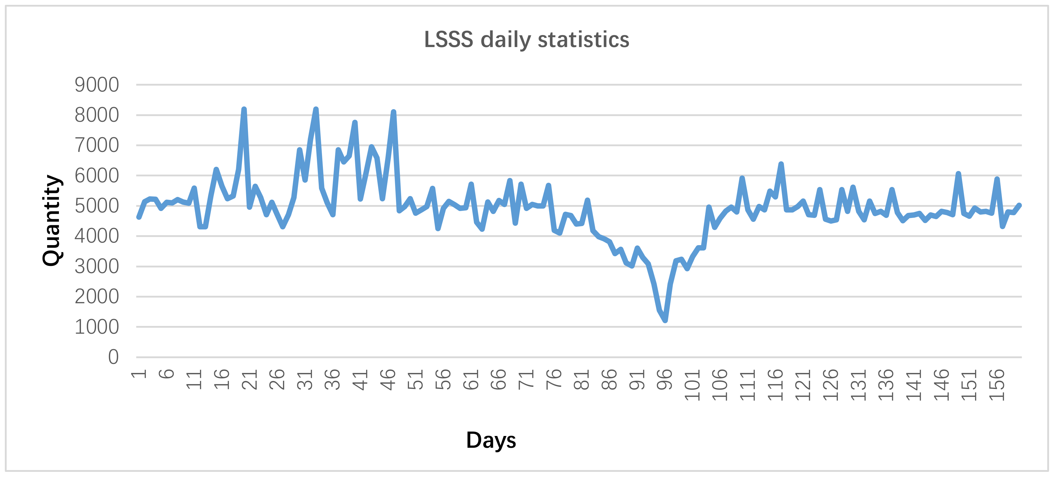
During the 183 days period from 12 November 2017 to 24 April 2018, a total of 787,283 people stayed in the Beijing underground rail transit system for a long time with an average of 4302 person-times per day (Figure 1). The trough in the picture occurred from 14 February to 23 February 2018. This trough occurs during the Spring Festival holiday. In China, there is a Spring Festival travel season, also known as ChunYun in Chinese. This is a special period when people who work far away from home return to their families in celebration of the Chinese Lunar New Year (the Spring Festival) [9]. LSSS is also the case, most of them went back home for the Spring Festival. In addition, without the Spring Festival holiday, the daily number of people who stay in the subway is predominantly stable. The number of passengers ranges between 4500 and 6000 and occasionally increases to 8000 in a few days, which is related to the traffic congestion caused by weather [10]. Some of the LSSS passengers are unintentional LSSS passengers (Intentional behavior means passengers do this deliberately to achieve a certain purpose. On the contrary, unintentional LSSS means that passengers are unwilling to do that, as for LSSS due to travelers missing a stop or being delayed. We think that if a passenger has very few LSSS(only one or two times), LSSS can be explained that travelers missing a stop or being delayed, it is a unintentional behavior; and if a passenger has a lot of LSSS, he must do it on purpose, it is an intentional behavior. In this paper, LSSS on purpose should be noticed, while unintentional LSSS should be ignored.) Unintentional LSSSs are normal behaviors, which are not subjects of our study. For the unintentional LSSS case, the passenger should not have LSSS four times in a week (the value is determined with subway operators). We cleared up the unintentional LSSS records.

Considering the period 12 November 2017 to 18 November 2017 as an example, 46,347 situations of LSSS occur in a week, including 27,068 LSSS card numbers. After removing unintentional factors, approximately 1000 people stayed in the subway for a long time in 1 week.

Several forbidden behaviors exist in the subway system, such as theft, begging and unauthorized advertisement. We analyzed the harmfulness of the behaviors as follow:

(1) Theft is an illegal and criminal act in any scene, which needs to be strictly prohibited. (2) Considering humanitarianism, begging behavior is acceptable, but the beggars in the subway are “professional beggars”. They are organized, large-scale and illegal. This kind of behavior seriously disturbs the order of passengers. When they are begging on the subway, passengers are not easily evacuated, which can easily cause a stampede. (3) Like begging, it is legal for unauthorized advertisement, but it is forbidden in the subway. If not handled properly, it will cause a stampede.

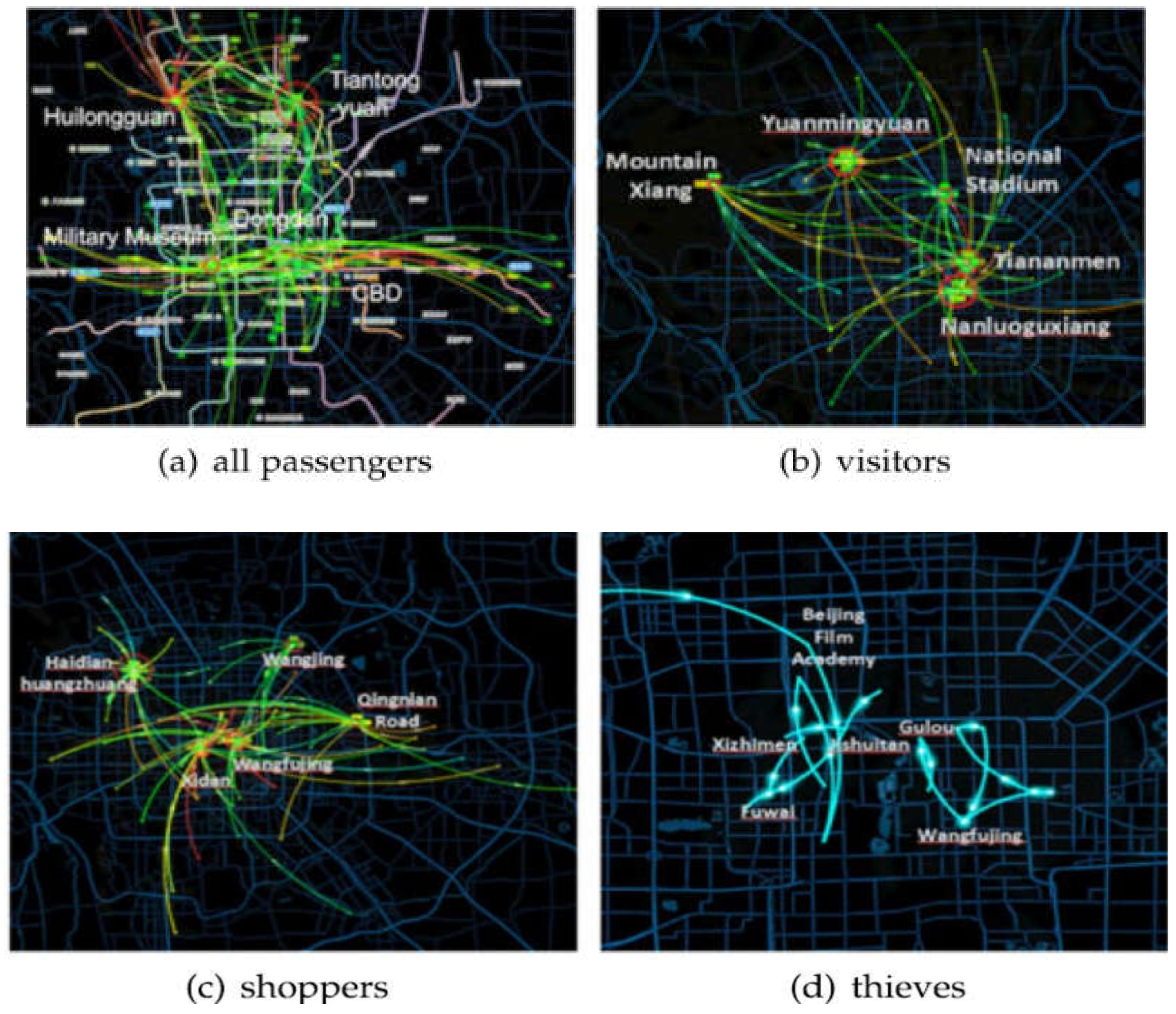
Public transit passengers can easily become distracted in crowded environments, because their focus drifts from their belongings, they often become common targets of pickpockets [7,8,11]. Du et al. [8] described the activity route of the pickpocket (Figure 2). Figure 3 and Figure 4 show some cases of the forbidden behaviors on Micro-blog. These prove that there are many abnormal passengers in the subway system. Based on literature and social media reviewing, and communication with rail transit safety experts, we summarize the characteristics of the three types of suspected abnormal behavior, as shown in

Table 1. Feature summary.

Type	Description
Suspected theft	Frequent rides in a certain period of time
	No distinct travel destination
	Transfer frequently
	Short trip
	Short ride time
Suspected begging	More fixed subway lines
	More stable begging route
	Very long ride time
Suspected unauthorized advertisement	More fixed time
	Frequent activities
	Very long ride time

[11,12,13,14,15]. The subway stays for a maximum of 4 h for the primary purpose to forbid the behavior of profit, begging [16]. If the card exceeds the time limit, the card cannot be used to exit the station. Even if a 4-h limit is issued, some people engage in acts of profit, begging, and advertising that endanger the safety and efficiency of rail transit operations. The subway operators and government agencies are not aware of the reasons for LSSS, if they stay in the subway for an extended period and perform some premeditated actions, this situation will not only hinder the interests of operators but also pose a substantial threat to the public safety.

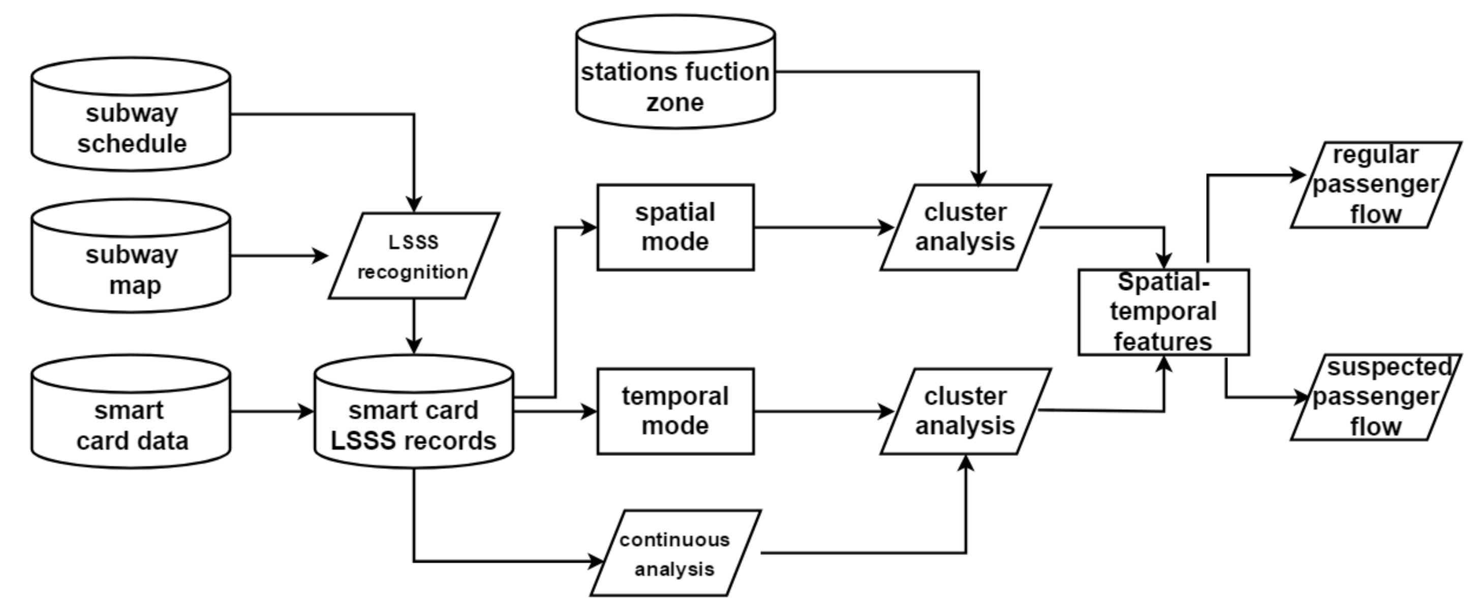
In this paper, we mine the temporal and spatial characteristics of LSSS and analyze the possibility of their behavior being abnormal. Then based on an assumed dataset of suspected abnormal passengers, we try to quantify the abnormal behaviors, and a SAE-DNN model is proposed to identify suspected abnormal passengers under the hypothesis. Figure 5 provides an overview of this paper.

2. Related Work

With the emergence of the Internet of Things technology in the era of big data, massive data are generated in urban operation management [2]. An increasing number of scholars have begun to study traffic data mining with tools such as data mining and machine learning. Pelletier et al. [2] concluded that the application of smart card data can be used for customer behavior analysis, timetable planning, and personal travel patterns. This paper focuses on such issues as travel behavior analysis, pattern mining and traffic anomaly analysis.

2.1. Travel Pattern Mining

Regarding travel behavior analysis and pattern mining, many scholars have investigated these issues in recent years. Ma et al. [3] (2013) proposed an effective data mining program that simulates the travel mode of Beijing passengers in Beijing and uses a K-Means ++ clustering algorithm and rough set theory to analyze travel patterns. Silva et al. [17] (2014) demonstrated that people’s travel patterns are predominantly spatial-temporal and predictable. Dabiri et al. [18] (2014) proposed a deep semi-supervised convolution auto encoder (SECA) architecture for travel pattern recognition, which not only automatically extracts relevant features from GPS segments but also utilizes unlabeled data. Tao et al. [19] (2014) used smart card data and flow-comap to check the spatial-temporal dynamics of bus passenger travel behavior; their research results can provide information for local public transport policies. Wang et al. [20] (2016) applied the LDA model to cluster the purpose of passenger travel in special areas; the results show that the model can identify users with different travel purposes and can determine the regular bus traffic demand and unconventional demand of commuters. Zhang et al. [21] (2016) proposed a new algorithm to identify the passenger mode by analyzing the event pattern and extracting the passenger’s transfer time and travel time using spatial-temporal information. The model was verified; the average estimation error is only approximately 15%. Medina [22] (2018) used discrete selection models to extract features from smart card data, applied DBSCAN clustering algorithms to these vectors, and estimated the likelihood of activity as HOME, WORK/STUDY or OTHER. Lu et al. [23] (2019) proposed a graph-based iterative propagation learning algorithm to identify visitors from public commuters and then designed a tourism preference analysis model to learn and predict their next trip. The literature [3,17,18,19,20,21,22,23] primarily analyzed the passenger’s travel mode from a spatial and temporal perspective.

2.2. Traffic Anomaly Analysis

Anomaly detection is a problem of finding outliers in the data. Till now, many anomaly detection techniques have been specifically developed for various applications. The techniques can be categorized as classification-based, distanced-based, clustered-based, and statistical-based, etc. Regarding traffic anomaly analysis, Lee et al. [24] proposed a partition and detect framework to detect outlying sub-trajectories from massive trajectory data. Ge et al. [25] provided an evolving trajectory outlier detection method by computing the outlying score for each trajectory in an accumulating way. Bu et al. [26] proposed an outlier detection framework for continuous trajectory streams. Pan et al. [27] (2013) described detected anomalies by mining representative terms from social media published by people at the time of the anomalies. Zheng [28] et al. (2014) established a trajectory model that simulated various group events and identified abnormal events, such as celebrations, marches, protests, and traffic congestion. Liu et al. [13] (2017) used a localized transportation mode selection model to identify areas with defective bus lines. Zhao et al. [29] (2017) defined the passenger’s travel mode from three aspects: spatial, temporal and spatial-temporal. Based on the clustering results, some marginal passengers were identified. The results were combined with the survey results, and a reasonable explanation of the abnormal travel characteristics of these passengers was provided. Public transport passengers are easily distracted in crowded environments, and they often become targets of pickpockets [7,8]. Du et al. [8] (2019) developed one suspected detection and surveillance system that identified pickpocket suspects based on their daily transit records.

3. Long-Term Staying in Subway System (LSSS) Recognition Model

Definition 1. 

A subway card contains the following information:

• t_route: Passenger’s route
• t_sboard: Passenger’s inbound station
• t_tboard: Passenger’s inbound time
• t_sexit: Passenger’s outbound station
• t_texit: Passenger’s outbound time
• t_ncard: Passenger’s card number
• t_mcard: Passenger’s card type
• t_ccard: Passenger’s card deduction
• t_bcard: Passenger’s card balance

From this information, we can calculate a passenger’s ride distance, ride time and the station and line that passed.

Definition2. 

A passenger’s ride information is a collection of all information in Definition 1:

T = (t1, t2..., tn)

where t = (t_route, t_sboard, t_tboard, t_sexit, t_texit, t_ncard, t_mcard, t_ccard, t_bcard)

t_ncard = 1–3 (ordinary card), 99–1 (Staff card), 99–19 (Student card)

Notations used throughout the paper are listed as follows and all boldface letters denote the corresponding vectors.

(1)

Indices

i	Line index, i = 1,2,…I

(2)

Parameters

L	theoretical time
M	the passenger transfer time in the subway
N	the actual time
O	the one ride boundary time
$D_i$	shortest distance in line i
$V_i$	represents technical speed of each line (Average speed of trains on each line)
$y_i$	whether the line i is passed or not, 1 means pass the line, 0 means not pass the line
$W_i$	waiting time for each line

Definition 3. 

The actual time of a passenger’s ride is the difference between the passenger’s outbound time and the inbound time.

Definition 4. 

The theoretical time of a passenger’s ride is the time required for the ride based on the shortest path algorithm with certain assumptions. The following series of assumptions are presented:

Hypothesis 1. 

The shortest path is selected when the passenger selects the transfer line.

Hypothesis2. 

Different subway lines have different speeds, and the speed of a train on each line is a fixed value.

Hypothesis 3. 

The $W_i$of different lines on the subway differs, and the$W_i$ is a fixed value.

Hypothesis 4. 

The theoretical time ($L$) of a passenger’s ride is calculated by the following formula:

$$L={\displaystyle \sum }_i^n\left(D_i/V_i\right)+{\displaystyle \sum }_i^n(y_i\times W_i)+[{\displaystyle \sum }_i^n(y_i)-1]\times M$$

(1)

Hypothesis 5. 

The passenger’s border travel time O rule is expressed as follows (

Table 2. Boundary Time Rule.

L	O
0–30 min	60 min
30–60 min	2$\times$L min
60–99999 min	∞ min

).

When the theoretical time of the ride is 0–30 min, the boundary time is 60 min. When the theoretical time of the ride is 30–60 min, the boundary time is two times the theoretical time. When the theoretical time of a ride is greater than 60 min, the boundary time is infinite. Due to the differences in the habits of different passengers, to avoid misjudging the normal passenger flow, we apply a strict definition of the abnormal duration, which may cause the omission of some LSSS but does not affect our research results.

Hypothesis 6. 

LSSS refers to the situation in which the actual time of a passenger exceeds the boundary time, N > O, N denotes to the actual time.

We determine these parameters based on experience and discussion with rail transit staff. Because of the lack of assurance, and in order to prevent misjudgment of some normal riders, the parameters we set are relatively strict. This may lead to some false negative riders, but false positive results will pose a threat to riders’ privacy, and therefore, the strict parameters are necessary.

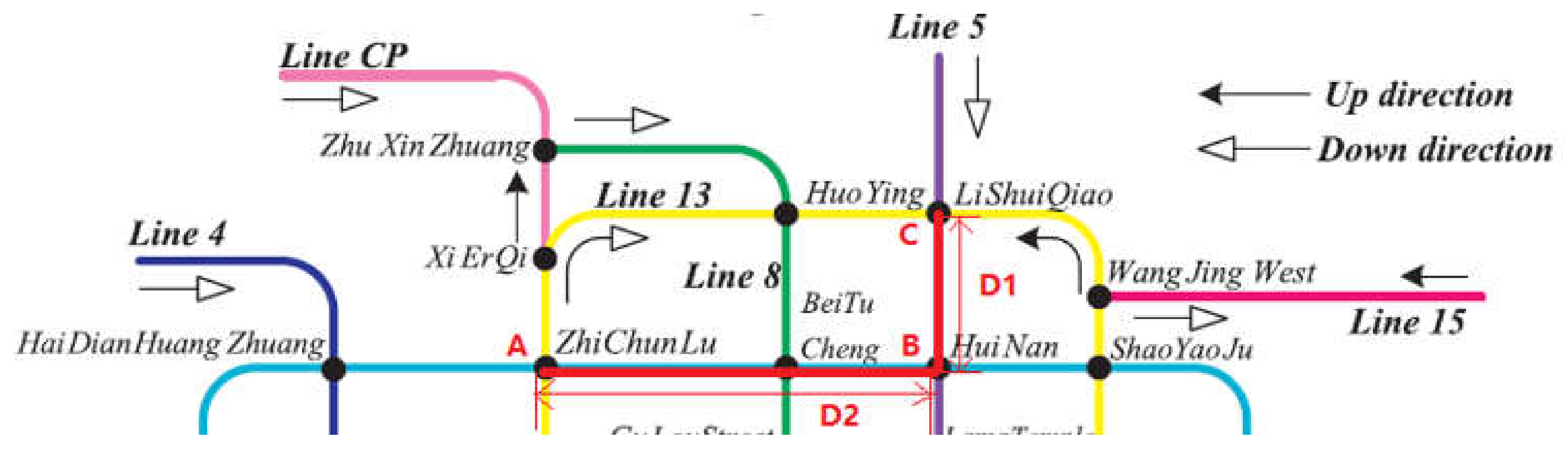
This is an example of calculating riding time for LSSS (Figure 6).

As for Figure 6, one ride is from stations A to C, the shortest path is calculated as A$\to$B, and then B$\to$C. The distance between B$\to$C is D1 and the distance between A$\to$B is D2. That is D_min,5 = D1, D_min,10 = D2; otherwise, D_min,I = 0. $y_5=1$ and$y_{10}=1$; otherwise, $y_i=0$.

D1 = 2.5 km, D2 = 5.5 km, $V_{line,5}$= 0.727 km/min, $V_{line,10}=0.755 \mathrm{km}/\min$, $T_{line,5}=2 \min$, $T_{line,5} = 3 \min$, $trt = 5 \min$

$$L=\frac{\mathrm{D}1}{V_{line,5}}+\frac{D2}{V_{line,10}}+T_{line,5}+T_{line,10}+M=\frac{2.5}{0.727}+\frac{5.5}{0.755}+2+3+5=20.72 \min$$

(2)

And then O = 60 min, if the passenger’s N is 65 min, this is an abnormal ride.

Five types of tickets are sold for the Beijing Subway: the outbound ticket, one-way ticket, ordinary stored value card, staff card, and student card. Each item of OD information has an identification code.

In this study, three types of noise data need to be eliminated:

• In the fare system, if the passenger does not have an IC card, he could buy a one-way ticket from station A to station B (assumed a price of 3 yuan). However, if he changes the destination from B to C during his trip (now his real route is A to C, assuming a price of 5 yuan), then the extra fee is needed (2 yuan); and an outbound ticket fee means the extra fee. This situation is inconsistent with the actual situation, which we aim to study in this article.
• Staff cards are used by staff members. They usually need to do maintenance work in the subway system and stay in the subway for a long time. Staff members have staff cards with a unique label, which can be distinguished from regular passengers.
• “In-Out” in the Same Subway Station refers to passengers entering and leaving at the same subway station. Passengers do not have spatial displacement, and this special phenomenon requires special research.

According to the previously discussed assumptions and definitions, the Floyd Shortest Paths Algorithm is imported. Data preprocessing and data cleaning environment is R language, and the solution environment is Python 3. This paper calculates the boundary time between the two stations of Beijing Subway, and the output of the model includes the actual time, theoretical time, passing line, passing station, and transfer times, as shown in

Table 3. LSSS solution results.

Start	To	Time	Transfer	Lines	Station	Stations
Andelibeijie	Andingmen	17	1	[‘line8’]	2	[‘Andelibeijie‘, ‘Guloudajie’, ‘Andingmen’]
Andelibeijie	Anhuaqiao	4	0	[‘line 8’]	1	[‘Andelibeijie’, ‘Anhuaqiao’]
…	…	…	…	…	…	…

. The OD data of the rail transit from 12 November 2017 to 24 April 2018 are divided into 22 slices in weekly units, and we separately solve the LSSS records, the results of the weekly solutions are highly consistent. We discover a total of 787,283 passengers’ actual time beyond the boundary time during 12 November 2017 to 24 April 2018. The research in the later sections of this paper is based on this result.

4. Temporal Model Based on LSSS

Temporal model based on LSSS means that this paper explores the sustainability of LSSS from three temporal dimensions, and then conducts Clustering Research on different persistent passengers. The model analyzes the characteristics of LSSS in time dimension, and finally extracts several typical time groups. Except for some special points caused by the weather, the characteristics of LSSS show strong consistency in different weeks, this paper considers the actual data of 1 week from 12 November 2017 to 18 November 2017, as an example and analyzes the data as follows, in which 46,347 situations of LSSS occur in a week, including 27,068 LSSS card numbers. The dataset of continuous LSSS Clustering includes 4752 records, and the rest of LSSS records are used in non-continuous LSSS Clustering.

4.1. LSSS Persistence Analysis

According to the statistics, LSSS has a substantial difference in the continuity of travel. To study the persistence of LSSS, this paper starts with the time data of three dimensions, namely, the time of passengers’ stay, the frequency of passengers’ rides and the inbound time distribution of passengers.

Most ride times in the subway are less than 2 h. The time does not seem long, but considering that the travel distance (only three to five stations without transfers), a typical ride is approximately 20 min. The time duration of the LSSS is far beyond the boundary time defined by the model, and the phenomenon of these passengers is extremely abnormal. Of all LSSS passengers, most of the timeouts range from 15–60 min, and most of these passengers have very few LSSS. Therefore, more than half of the stay behavior may not be attributed to the intentional willingness of the passenger but may be attributed to a wrong route, missed stop, and temporary change in travel route. The previously mentioned users are not within the scope of LSSS research. Therefore, this paper excluded these LSSS records.

We define a user’s intentional LSSS in such a way that the user has four or more occurrences of LSSS in a week. If this phenomenon occurs during the week, a passenger’s LSSS behavior will be recorded one time, and then we count the LSSS weeks of each user. The proportion of passengers who had a single-week LSSS phenomenon and then disappeared exceeds 50%, while the proportion of users who have LSSS for more than 3 consecutive weeks accounts for only approximately 10%. We divide intentional LSSS into continuous LSSS (continuous behavior for more than 3 weeks) and non-continuous LSSS to study passenger preference in temporal mode.

4.2. Continuous LSSS Clustering Analysis

To study the distribution of continuous LSSS in various time periods during the day, we will divide the distribution into a time period every 3 h. The time periods H1, H2...H7 represent 3:00:00–6:00:00, 6:00:00–9:00:00…21:00:00–24:00:00 (0:00:00–3:00:00 no subway departure). Unsupervised clustering algorithms are often used to classify travel patterns [3,14].

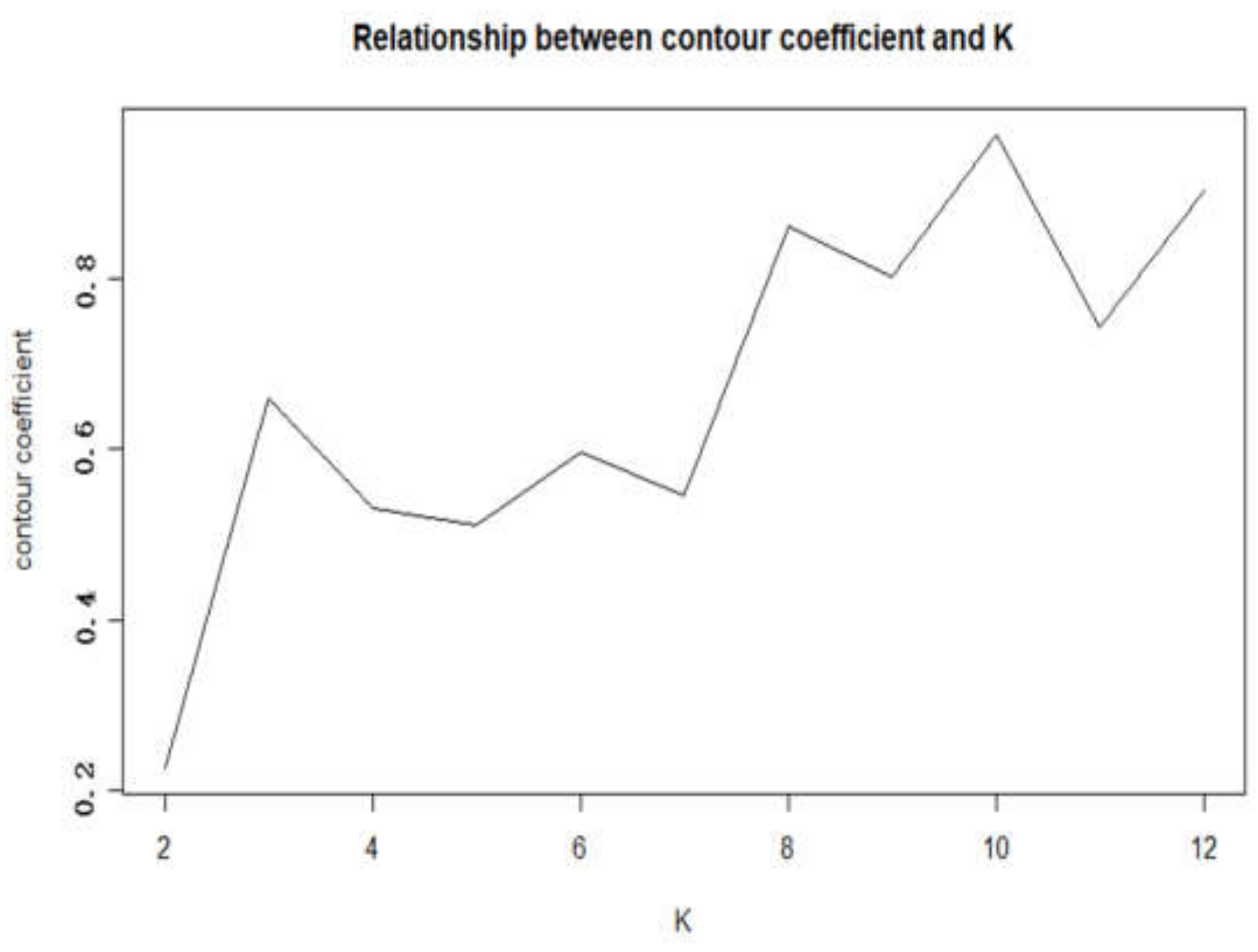
Silhouette Coefficient is an evaluation metric of a clustering algorithm. The silhouette coefficient $s_i$ is calculated by $s_i=b_i-a_i/\max \left(a_i,b_i\right)$ where $a_i$ is the average dissimilarity of the ith passenger with all other passengers within the same cluster. $b_i$ is the lowest average dissimilarity of ith passenger to any other cluster. The silhouette coefficient is in [−1, 1], where a large value indicates that the passenger is well matched to the cluster and poorly matched to others. We compare the silhouette coefficient of k-means, DBSCAN and Hierarchical methods; k-means algorithm is the suitable one for this problem. A K-means cluster analysis was performed using the number of inbound recordings of each passenger in the seven time periods as variables.

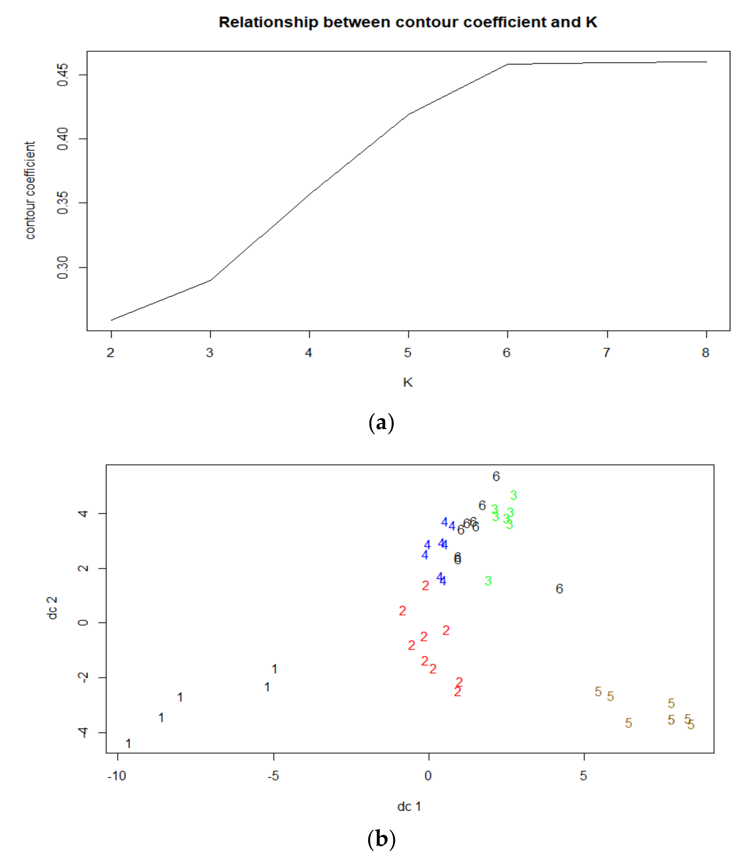
As shown in Figure 7a, when K = 6, the Silhouette Coefficient reaches the maximum. We gathered these passengers into six categories: CTGrp1, CTGrp2, CTGrp3, CTGrp4, CTGrp5, and CTGrp6. And Figure 7b shows the distribution of classes, because of the limitation of space, we selected some samples to show in the figure. The cluster center points of these six types of passengers are shown in

Table 4. Continuous LSSS Clustering Center.

Type	H1	H2	H3	H4	H5	H6	H7	Percent
CTGrp 1	0	0	29.2	5.2	0.8	0.4	0.6	10.8%
CTGrp 2	5	5.8888	5.5555	2.3333	1.8888	2.1111	1.44444	19.5%
CTGrp 3	0	1.7142	1.1428	29.7142	4.7142	2.7142	0.28571	15.2%
CTGrp 4	0	0.625	1.75	2.875	6	24.75	2.375	17.3%
CTGrp 5	0	37.375	0.375	0.25	0.625	0.125	0	17.3%
CTGrp 6	0	1.777	0.33333	1.5555	29.444	2.333	0.1111	19.5%

H1, H2…H7 represent 3:00:00–6:00:00, 6:00:00–9:00:00 …21:00:00–24:00:00 (0:00:00–3:00:00 no subway departure). The values in Hi columns denote the average passenger numbers of the type CTGrp j in Hi time period. Percent column denotes the proportion of the type CTGrp j in total samples. And the bold denotes to active point of the passenger.

.

The inbound times of CTGrp1 passengers are concentrated from 9:00:00–12:00:00; the inbound times of CTGrp3 passengers are concentrated from 12:00:00–15:00:00; and the inbound times of CTGrp6 passengers are concentrated from 15:00:00–18:00:00. In addition, the inbound times of CTGrp4 passengers and CTGrp5 passengers are concentrated in the morning or evening peaks. These five categories of passengers have only 1 peak hour of travel, while long-term stable commuter passengers usually contain round-trip OD pairs. Thus, these five types of passengers are not regular commuters; they are “special personnel” who work at fixed times. The CTGrp2 passengers do not have a stable inbound time; they act like people who wander in the subway. With caution, we suspect that they are suspected of being thieves.

4.3. Non-Continuous LSSS Clustering Analysis

The Non-continuous LSSS is the residual LSSS that removes the continuous LSSS, which is considerably larger in number than the continuous LSSS. These passengers may occasionally have occurrences of LSSS for 1 to 2 weeks for work or other reasons. They may need to change the card number to avoid tracking by big data. We perform a passenger cluster analysis based on the inbound records for the H1–H7 time period. The results are presented as follows:

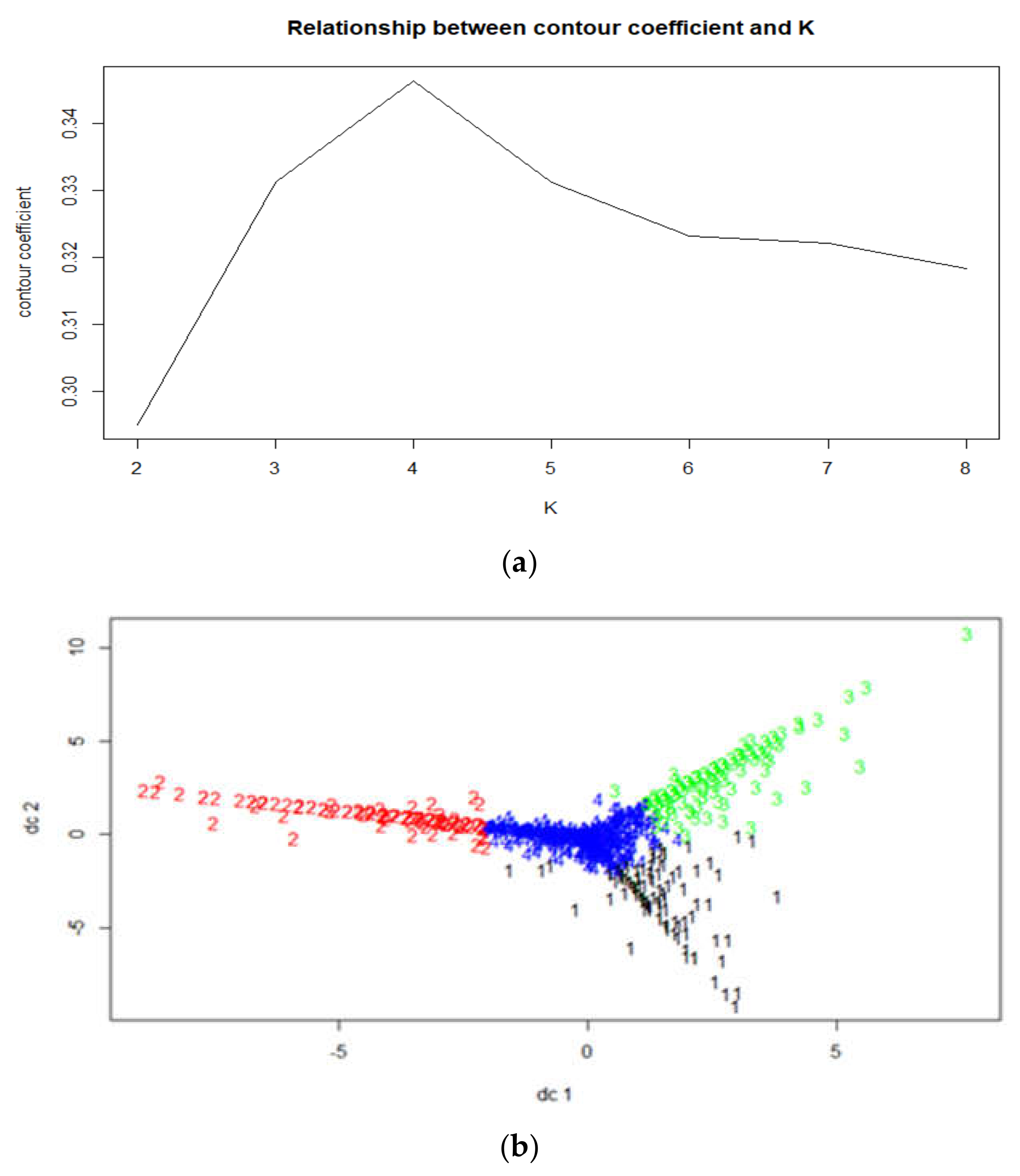
As shown in Figure 8, when K = 4, the Silhouette Coefficient is the largest. Thus, the non-continuous LSSS is clustered into four categories: N-CTGrp1, N-CTGrp2, N-CTGrp3, and N-CTGrp4. And Figure 8b shows the distribution of classes. The cluster center points are shown in

Table 5. Non-continuous LSSS Clustering Center.

Type	H1	H2	H3	H4	H5	H6	H7	Percent
N-CTGrp 1	0.034	0.401	0.1282	0.5811	17.017	1.5982	0.0940	11.9%
N-CTGrp 2	0.133	16.266	0.7733	0.2866	0.5333	0.1933	0	15.3%
N-CTGrp 3	0	0.171	0.2808	0.1438	1.8493	13.7671	0.73287	14.9%
N-CTGrp 4	0.621	1.808	2.6690	1.9911	1.76106	0.98938	0.52389	57.7%

H1, H2…H7 represent 3:00:00–6:00:00, 6:00:00–9:00:00 …21:00:00–24:00: 00 (0:00:00–3:00:00 no subway departure). The values in Hi columns denote to the average passenger numbers of the type N-CTGrp j in Hi time period. Percent column denotes the proportion of the type N-CTGrp j in total samples. And the bold denotes to active point of the passenger.

.

The common characteristics of the first three types of passengers are described as follows: the existence of only 1 inbound peak hour; the inbound stations are concentrated at 15:00:00, 6:00:00, and 9:00:00; and the proportions in the total non-continuous passenger flow are similar; they range between 10% and 15%. Similar to several types of passengers in continuous LSSS, commuting behavior does not exist. N-CTGrp4 does not have distinct inbound peaks and includes purposeless wandering passengers.

By comparing the clustering results of continuous and discontinuous LSSS, we discovered that the two clustering results are similar to the whole set of results. For example, many types of passengers represent single inbound peaks; a class of passengers enters the station with chaotic times.

The difference is that the centralized period of continuous LSSS is more dispersed, while the non-continuous LSSS is only concentrated in three periods. The number of intricate paths in the non-continuous LSSS is substantially higher than that in the continuous LSSS. A larger number of chaotic riders tend to hide their travel data, which prevents the tracking of big data.

5. Spatial Model Based on LSSS

Spatial based on LSSS means that this paper first divides each station into different categories according to their functions. Then, according to the preference of LSSS’s function area, the model makes cluster analysis, and finally extracts several typical spatial groups. LSSS Clustering Analysis based on Spatial Model and Functional Area Classification uses the actual data of 1 week from 12 November 2017 to 18 November 2017, as an example and analyzes the data as follows, in which 46,347 situations of LSSS occur in a week, including 27,068 LSSS card numbers.

5.1. Subway Station Functional Area Classification

In order to explore the law of LSSS in geospatial space, this paper classifies the functional areas of various stations in Beijing, which helps to understand the subway LSSS features on spatial patterns.

Most of the research on the classification of subway stations considered the urban built-up area as the research object and the suburban subway station as a sub-category (Korf et al., 1981) [30]. Chinese scholars have not yet formed a unified understanding of the classification method for subway stations. The main classification methods are described as follows: The first method is the standard adopted by some cities in China’s about urban subway construction; the second method is classifying according to the land-use near the station, that is, according to the location characteristics of the subway station; the third method is classifying by the rail transit operation data; and the fourth method is the microscopic urban spatial form based on the station [31]. Because this research examines passenger travel patterns, the classification of subway stations from the perspective of passenger travel characteristics is more suitable for the research. Yin Qin et al. [31] (2016) employed the time series clustering method with passenger flow characteristics to classify the 195 subway stations in Beijing. Tan [32] et al. performed feature factor extraction and station type identification using smart card data of 136 subway stations in Guangzhou. Chen et al. [33] (2018) extracted five main factors from the variables and the main factors to cluster the stations. By the K-means clustering method, the subway station of Shanghai Metro Line 359 is divided into several types of stations with different congestion levels. This paper quotes the results of Yin Qin et al. [31] and combines the research results of Tan [34] to fine-tune the results of the station; the metro stations are divided into 10 categories.

5.2. LSSS Clustering Analysis Based on Spatial Model and Functional Area Classification

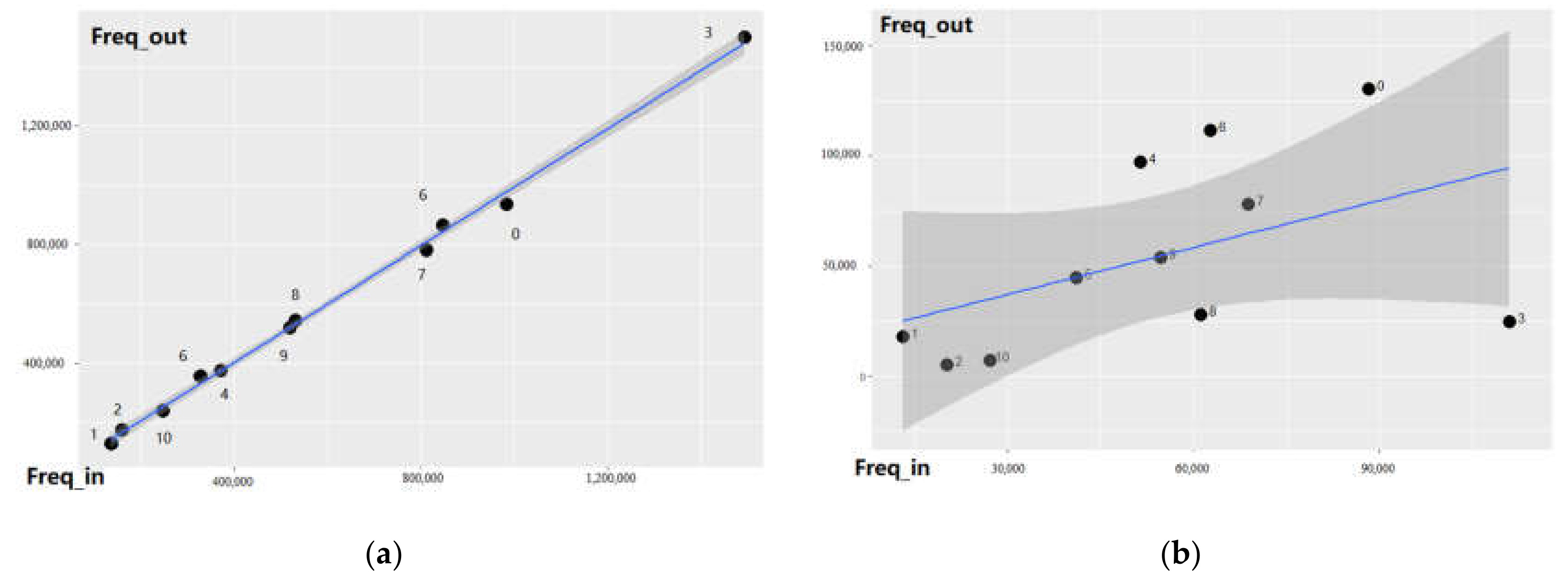
Each station is matched with the corresponding functional area. Figure 9 left shows the functional area OD pairs of the regular passenger flow; the abscissa is the inbound frequency of the i-function zone; and the ordinate is the outbound frequency of the i-function zone. Each point in the figure is near the y = x asymptote, as observed in the functional areas of the regular passenger flow, which are very balanced. However, the distribution of the LSSS passenger’s functional area inbound and outbound OD pairs (Figure 9b) is very different. The LSSS inbound station prefers the misplaced area and the transportation hub area, while the outbound station prefers the misplaced biased residential stations, the mixed-type stations and other stations.

To study the preference of LSSS in each functional area, we select the frequency of each passenger’s entry and exit in 10 functional areas as a clustering index and perform a K-means cluster analysis for users who make more than 10 rides in half a year.

As shown in Figure 10, when K = 10, the Silhouette Coefficient attains the maximum. Thus, the best classification is 10, SGrp1, SGrp2…SGrp10. We determined that the proportion of more than 60% has a distinct functional zone preference. SGrp2, 3, 5, and 7 have only a distinct preference in the inbound functional area, and the outbound station distribution is random. For SGrp4 6, 8 and 9, only the function area of the outbound station has a distinct preference, and the inbound station is randomly distributed. The SGrp1′s inbound station and the outbound station both have distinct preferences. The SGrp10 passengers are distributed in each functional area without a distinct preference. Except for SGrp10, each category has a single area preference (inbound function area or outbound function area) on the functional area. Most of the LSSS routes are fixed, and we extract each type’s high-frequency functional area. The preferences are shown in

Table 6. Spatial clustering results.

SGrp	In	Out	Percent	SGrp	In	Out	Percent
1	Misplaced biased residence	Misplaced biased residence	8.5%	6	None	Misplaced biased residence	13.3%
2	Employment-oriented	None	4.39%	7	Mixed type	None	6.1%
3	Position misplaced	None	14.5%	8	None	Comprehensive	11.9%
4	None	Other	13.9%	9	None	Comprehensive	9.1%
5	Scenic type	None	4.5%	10	None	None	13.1%

.

Regardless of the type, none of the passengers prefer residential functional areas; thus, we can infer that these LSSS passengers are not commuters. For SGrp1, they tend to misplace the biased residence station. Most of these stations are Shunyi, Xihongmen and other places; they are located at the edge of the city and belong to the beginning or end of the subway line.

SGrp2, 3, 5, and 7 have fixed preferences on the entry station, with SGrp5 entering the station that tends to the tourist zone, and SGrp2, 3, and 7 prefer the employment-oriented zone. Their outbound stations are complex, which increases their likelihood of suspected distributing advertising behaviors.

SGrp4, 6, 8, and 9 have fixed preferences on the outbound station, with SGrp4, 8, and 9′s outbound stations preferring the comprehensive and mixed zones, while SGrp6 outbound stations are more likely to be misplaced biased residence. Although the types have distinct tendencies, evidence of their purpose does not exist.

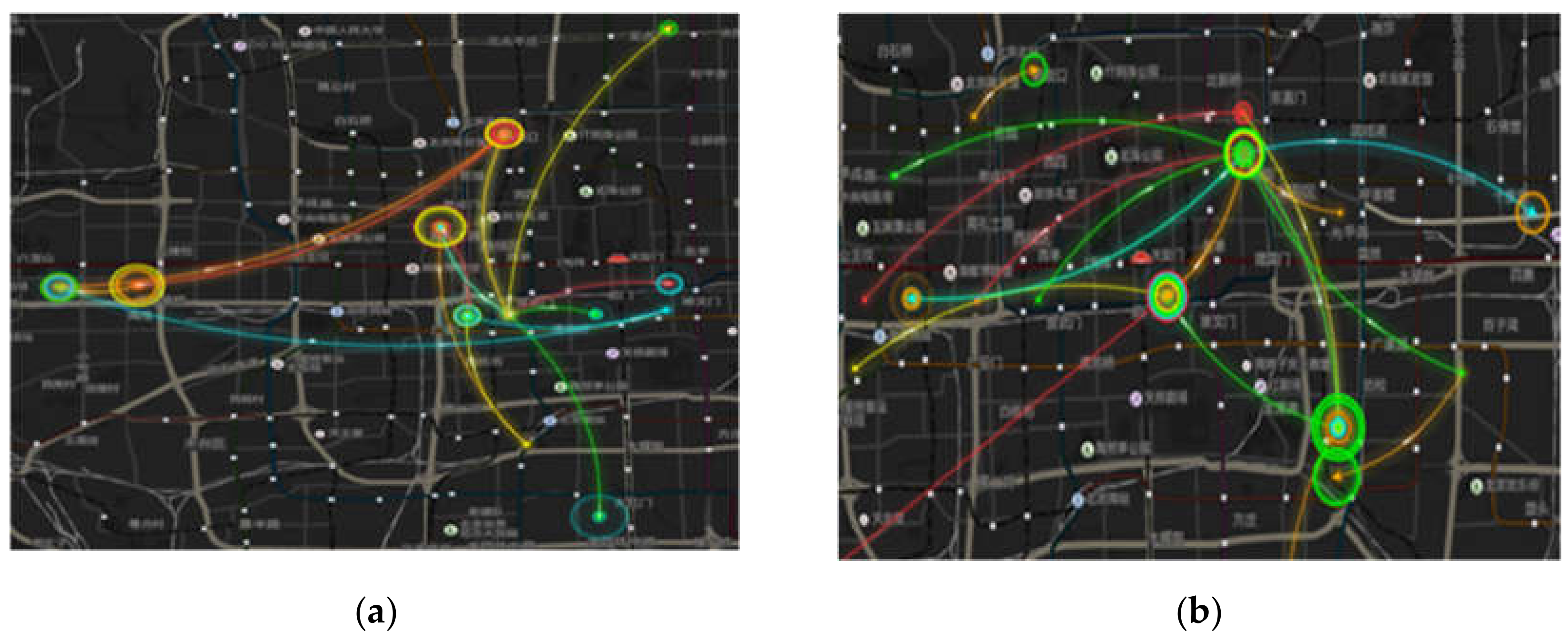
For SGrp10, these passengers have no station preference and the lines are intricate, as shown in Figure 11. Their most prominent feature is that they wander purposelessly. According to literature [8], suspected passengers of each travel purpose have unique fixed characteristics. The spatial characteristics of this type of passenger are consistent with the paths of suspected thieves.

6. Identification Method of Anomaly Riders

6.1. Identification Problem

In order to identify the suspected anomaly riders, we try to qualify the anomaly behavior based on the riding records and above analysis, and propose a model to identify the anomaly behavior, which could reduce the risk of subway system. Suppose the subway network is $G=\left(S, E\right)$, where $S=\left\{s_1,s_2, . . . , s_N\right\}$is the set of stations, and N is the number of stations. $\left(s_i,s_j\right)\in E$ denotes the OD (Origin-Destination) path from station $s_i$ to $s_j$, where $s_i$ is termed as origin station, and $s_j$ is destination station. Given a passenger IC card, a set of OD paths with inbound and outbound time are obtained, and the model extracts the a spatial-temporal feature vector of the rider. Finally, the anomaly rider is identified by the SAE-DNN framework.

6.2. Anomaly LSSS Feature Vector Extraction

It has been proved above that the travel of suspected anomaly people has obvious characteristics both temporal and spatial. If the passenger’s valid travel feature vector can be extracted, the suspected anomaly behavior can be supervised and identified. Du et al. [8] built a suspected pickpocket training set from Travel Time and Frequency and achieved good results.

This paper considers that suspected beggars like to live in the fringe area of the city, and suspected thieves like to haunt in densely populated areas. We divide 358 subway stations into four functional areas based on people’s general perception and passenger flow distribution. That is: urban fringe (M), urban core (C), transportation hub (T) and other stations (O). From this, the OD matrix PM_i of each passenger can be constructed:

$$P{M}_i=\begin{array}{ccccc}& M& C& T& O\\ M& P_{i\left(1,1\right)}& P_{i\left(1,2\right)}& P_{i\left(1,3\right)}& P_{i\left(1,4\right)}\\ C& P_{i\left(2,1\right)}& P_{i\left(2,2\right)}& P_{i\left(3,2\right)}& P_{i\left(2,4\right)}\\ T& P_{i\left(3,1\right)}& P_{i\left(3,2\right)}& P_{i\left(3,3\right)}& P_{i\left(3,4\right)}\\ O& P_{i\left(4,1\right)}& P_{i\left(4,2\right)}& P_{i\left(3,4\right)}& P_{i\left(4,4\right)}\end{array}$$

(3)

For example, the input of machine learning models such as regression, decision tree, and SVM should be vectors instead of matrices. We do the following processing to get PV_i:

$$P{V}_i=\begin{array}{ccccccc}M\to \mathrm{M}& M\to \mathrm{C}& M\to \mathrm{T}& M\to \mathrm{O}& \dots & O\to \mathrm{T}& O\to \mathrm{O}\\ P_{i\left(1,1\right)}& P_{i\left(1,2\right)}& P_{i\left(1,3\right)}& P_{i\left(1,4\right)}& \dots & P_{i\left(3,4\right)}& P_{i\left(4,4\right)}\end{array}$$

(4)

In the time dimension, we consider two aspects, one is the distribution of the travel time period, such as suspected beggars like to take action at noon and afternoon, and suspected thieves like to haunt in the morning and evening peaks. Another indicator is the distribution of travel time. For example, suspected beggars will stay in the subway for a long time, and suspected thieves often have shorter pit stops. To this end, we divide the day into four time periods: morning, noon, afternoon, and evening. The ride duration is divided into five time periods: 0–15, 15–30, 30–60, 60–120, and 120–∞. Passenger time feature vector PT_i:

$$P{T}_i={\begin{array}{ccccccccc}\mathrm{Morning}& \mathrm{Noon}& \mathrm{Afternoon}& \mathrm{Evening}& 0\to 15& 15\to 30& 30\to 60& 60–120& 120\to \infty \\ P_{i,M}& P_{i,N}& P_{i,A}& P_{i,E}& P_{i,15}& P_{i,30}& P_{i,60}& P_{i,120}& P_{i,\infty }\end{array}}_{ }$$

(5)

The Spatial-temporal feature vector P_i of a passenger is (PV_i, PT_i).

An imbalanced data set means that the sample size of each category of the data set is extremely uneven. Taking the binary classification problem as an example, it is assumed that the number of samples of the positive class is much larger than that of the negative class. The data in this case is called imbalance data. Obviously, In the identification model of regular passenger flow and suspected anomaly passenger flow, the sample of suspected anomaly prediction is an imbalanced data set. We apply naive random under sampling method to process regular passenger data.

6.3. A Deep Neural Network with Stacked Autoencoders (SAE-DNN)

In this paper, we build a deep neural network with a stacked autoencoders (SAE-DNN) model for suspected anomaly recognition. In the SAE stage, we can conduct a feature extraction about the feature vector, and input the trained weight into DNN, which could improve the accuracy of suspected anomaly detection.

An autoencoder is an artificial neural network used for unsupervised learning of efficient coding [35]. It was first introduced in the 1980s by Hinton and the PDP group [36] to address the problem of ‘‘back propagation without a teacher”, by using the input data as the teacher [37]. Recently, autoencoders have been more widely used for learning generative models of data [38].

It typically has an input layer that consists of the input vector X, one or more hidden layers which consist of the transformed feature vector H defined as an encoder shown in Equation (6), and an output layer which consists of the reconstruction vector R defined as a decoder shown in Equation (10). $\delta$ and $\tilde{\delta }$ denote the linear and weighted combinations shown in Equations (7) and (8), respectively. The output vectors should match the input vectors, which have the same dimensionality and values similar to those of the input vectors. T(·) is the activation function. We apply tanh and rectifier as the activation functions shown in Equations (10) and (11), respectively [36].

$$H=f\left(X\right)=T\left({\displaystyle \sum }_i{w}_i{x}_i+b_i\right)$$

(6)

$$R=g\left(X\right)=T\left({\displaystyle \sum }_i\widetilde{w_i}{h}_i+\widetilde{b_i}\right)$$

(7)

$$\delta ={\displaystyle \sum }_i{w}_i{x}_i+b_i$$

(8)

$$\tilde{\delta }={\displaystyle \sum }_i\widetilde{w_i}{x}_i+\widetilde{b_i}$$

(9)

$$Tanh\left(\alpha \right)=\frac{e^{\alpha }-e^{-\alpha }}{e^{\alpha }+e^{-\alpha }}$$

(10)

$$Rectifer\left(\alpha \right)=\max \left(0,\alpha \right)$$

(11)

where input vector X is a set of training datasets {x₁, x₂, x₃,…, x_n}; H is a set of encoders {h₁, h₂, h₃,…, h_n}; R is the a set of reconstruction results {r₁, r₂, r₃,…, r_n}; f(X) is the encoder function with weight (w_i) and bias (b_i); g(H) is the decoder function with weight ($\widetilde{w_i}$) and bias ($b_i$); and $\alpha$ denotes $\delta$ or $\tilde{\delta }$.

Equation (12) is used to minimize the reconstruction error between the input vector X and the reconstruction vector R.

$$L\left(X,R\right)=minL\left(X,R\right)$$

(12)

In order to make the reconstruction results R match the input vector X; the loss function L(X,R) should be minimized by fine-tuning the parameters of $w_i$ and $b_i$ shown in Equations (13) and (14).

$$w_i{}^{’}=w_i-\eta \frac{\partial L\left(x_i,r_i\right)}{\partial w_i}$$

(13)

$$b{i}^{’}=bi-\eta \frac{\partial L\left(x_i,r_i\right)}{\partial bi}$$

(14)

where $w_i$ and $w_i{}^{’}$ are the original weight and updated weight for the ith node in each hidden layer; $bi$ and $b{i}^{’}$ are the original bias and updated bias for the ith node in each hidden layer; and $\eta$ is the learning rate.

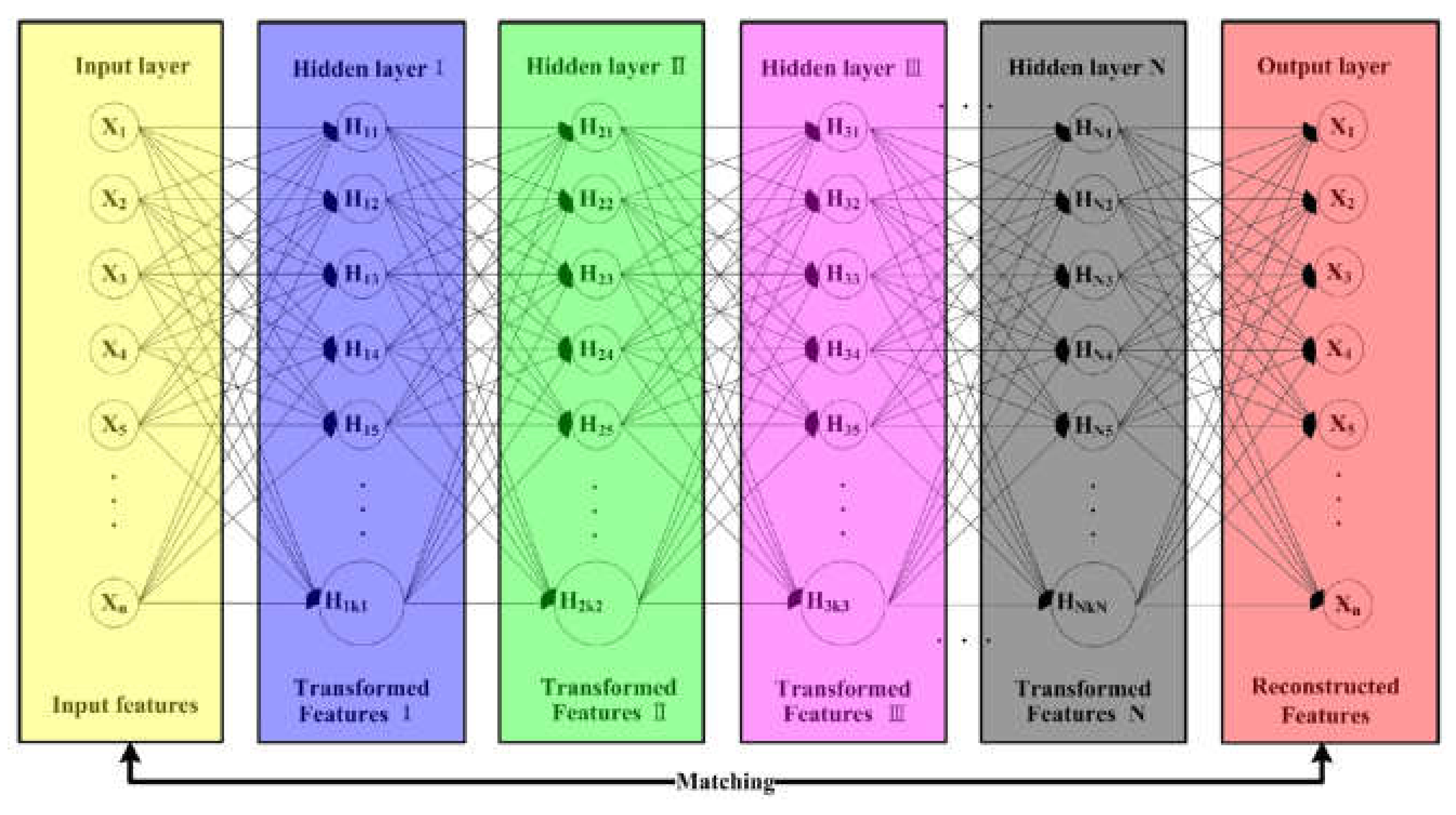
Autoencoders can be stacked to form a deep network to obtain an abstract representation of the input through gradual feature extraction, known as a SAE. The structure of a SAE is shown in Figure 12. The blue, green, purple, and grey backgrounds represent the first hidden layer, the second hidden layer, the third hidden layer, and the Nth (last) hidden layer, respectively. The number of nodes in each hidden layer is kn (n = 1, 2...N).

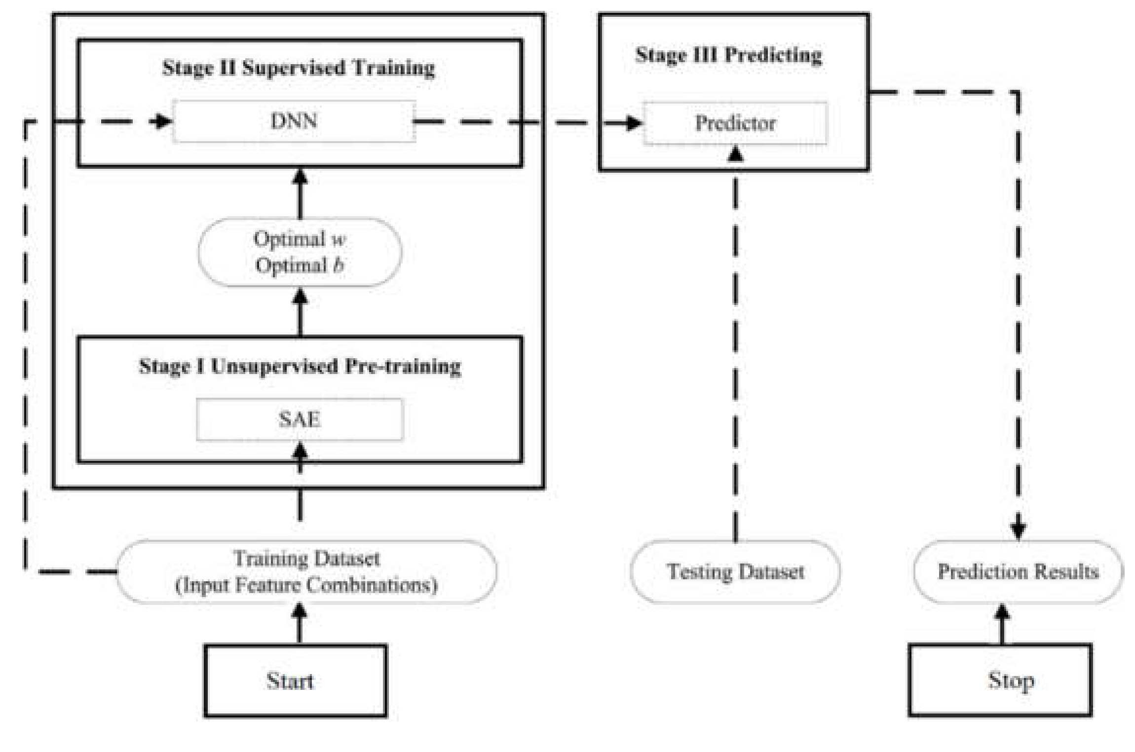
Figure 13 shows the structure of the SAE-DNN. The training and predicting procedures of a SAE-DNN consist of three stages. In the first stage, we pre-train the greedy layer-wised SAE by using a purely unsupervised approach with different features combined as different training datasets. The SAE is used to initialize the weights and bias for the DNN. In the second stage, the supervised DNN with the label data is conducted. The final stage predicts the category of passengers. The feed-forward and back-propagation algorithms are based on the literatures. Detailed explanations of the training and predicting procedures in the three stages are shown in Algorithm 1 [39].

Algorithm 1

Stage I: SAE for an unsupervised pre-training. Input: (1) Training dataset X = {xij}, i is the number of unsupervised input examples, j is the number of unsupervised input features; (2) One input layer, one output layer, and N hidden layers; (3) Number of nodes in each hidden layer: kn (n = 1, 2…N); (4) Stop threshold: $\theta$. Step 1: Initialize the parameters (w, b) in all layers (N + 2) randomly. Step 2: Layer-wise train all nodes in all hidden layers. The training process in each layer includes the following four steps. (1) Encode every node by Equations (6), (8) and (10); (2) Decode every node by Equations (7), (8) and (10); (3) Compute the reconstruction error L(X, R) by Equation (12); (4) Back-propagation algorithm: If (L(X, R) >$\theta$) Minimize the reconstruction error L(X, R) by Equations (13) and (14), go to Step 2(1); Else end. Step 3: Repeat Step 2 until all the hidden nodes in all hidden layers have been trained. Output: The pre-trained SAE. Stage II: DNN for a supervised training. Input: (1) The pre-trained SAE; (2) Training dataset X = {xij’}, i is the number of supervised input examples, j’ is the number of supervised input features; (3) One input layer, one output layer, and N’ hidden layers; (4) Number of nodes in each hidden layer: kn (n = 1, 2…N’); (5) Stop threshold: ${\theta }^{\prime }.$ Step 4: Use the SAE to initialize the parameters (w’, b’) for all layers (N’ + 2). Step 5: Train all nodes from the input layer to output layer with the assumed passenger type as the label data. It includes the following three steps. (1) Train every node with the feed-forward algorithm by Equations (6), (8) and (11) layer to layer, and get the output Y in the (2) output layer; (3) Compute the error L(X, Y) between the input in the first input layer and the output in the last output layer by Equation (9); (4) Back-propagation algorithm: If (L(X, Y) > ${\theta }^{\prime }$) Minimize the error L(X, Y) by Equations (13) and (14), go to Step 5(1); Else end. Output: The trained model (predictor). Stage III: Predicting. Input: (1) Testing dataset T = {tmj}, m is the number of testing examples, j is the number of input features; (2) Predictor. Step 6: Input T into the predictor. Step 7: Perform the prediction. Output: Prediction type.

7. Experimental Results

7.1. Anomaly LSSS Samples

The datasets consist of the Beijing Subway OD data from 12 November 2017 to 24 April 2018, with approximately 75 million effective travel records. OD traffic refers to the amount of traffic between the start point and the end point. “O” is derived from the English ORIGIN, which indicates the starting point of the line, and “D” is derived from the English DESTINATION, which indicates the destination of the line.

From the temporal mode analysis, the subway LSSS can be divided into continuous LSSS and discontinuous LSSS. The two types are similar in some respects. From the clustering results, we determine that the total LSSS can be summarized into two categories in the inbound time dimension: A: Inbound time stable; B: Inbound time unstable. Combined with the station functional area classification, the spatial pattern can show the passenger’s preference, and the passengers are clustered into 10 categories. To highlight the differences in passengers in the spatial model, we merge the types that are similar. Passengers are divided into four categories in spatial mode: (A): Inbound and outbound stations are stable, (B): Inbound stable type, (C): Outbound stable type, and D: Inbound and outbound stations are irregular.

We counted the classification of each passenger in temporal mode and spatial mode. X_Y represents the passenger classified as X in temporal mode, the passenger classified as Y in spatial mode, and the classification of passengers, as shown in

Table 7. Spatial clustering results.

Type	A_A	A_C	A_D	B_B	B_D
Freq	28.65%	44.38%	8.99%	11.24%	6.74%

and

Table 8. Temporal and spatial comprehensive classification.

Type	A_A	A_C	A_D	B_B	B_D
Suspected behavior	suspected begging	suspected unauthorized advertisement	suspected theft	suspected unauthorized advertisement	suspected theft

. After checking the characteristics one by one with the rail transit safety experts, some LSSS passengers with low similarity to suspected abnormal behaviors were eliminated. After serious judgment, we obtained the most suspected passengers (158 in total, training set includes 110 samples and testing set includes 48 samples; the division method is random division).

7.2. Results

The evaluation metrics are Logarithmic Loss metric:

$$LogLoss=-1/n{\displaystyle \sum }_{i=1}^n\left[g{t}_i\log \left(p_i\right)+\left(1-g{t}_i\right)\log \left(1-p_i\right)\right],$$

(15)

where $g{t}_i$ denotes the ground truth of rider i, and $p_i$ is the probability returned by a system that the identification result of rider i is true.

$$Acc=\frac{TP+TN}{TP+TN+FP+FN},$$

(16)

where $TP \mathrm{and} FP$ denote True Positive and False Positive;$TP \mathrm{and} FN$ denote True Positive and False Negative.

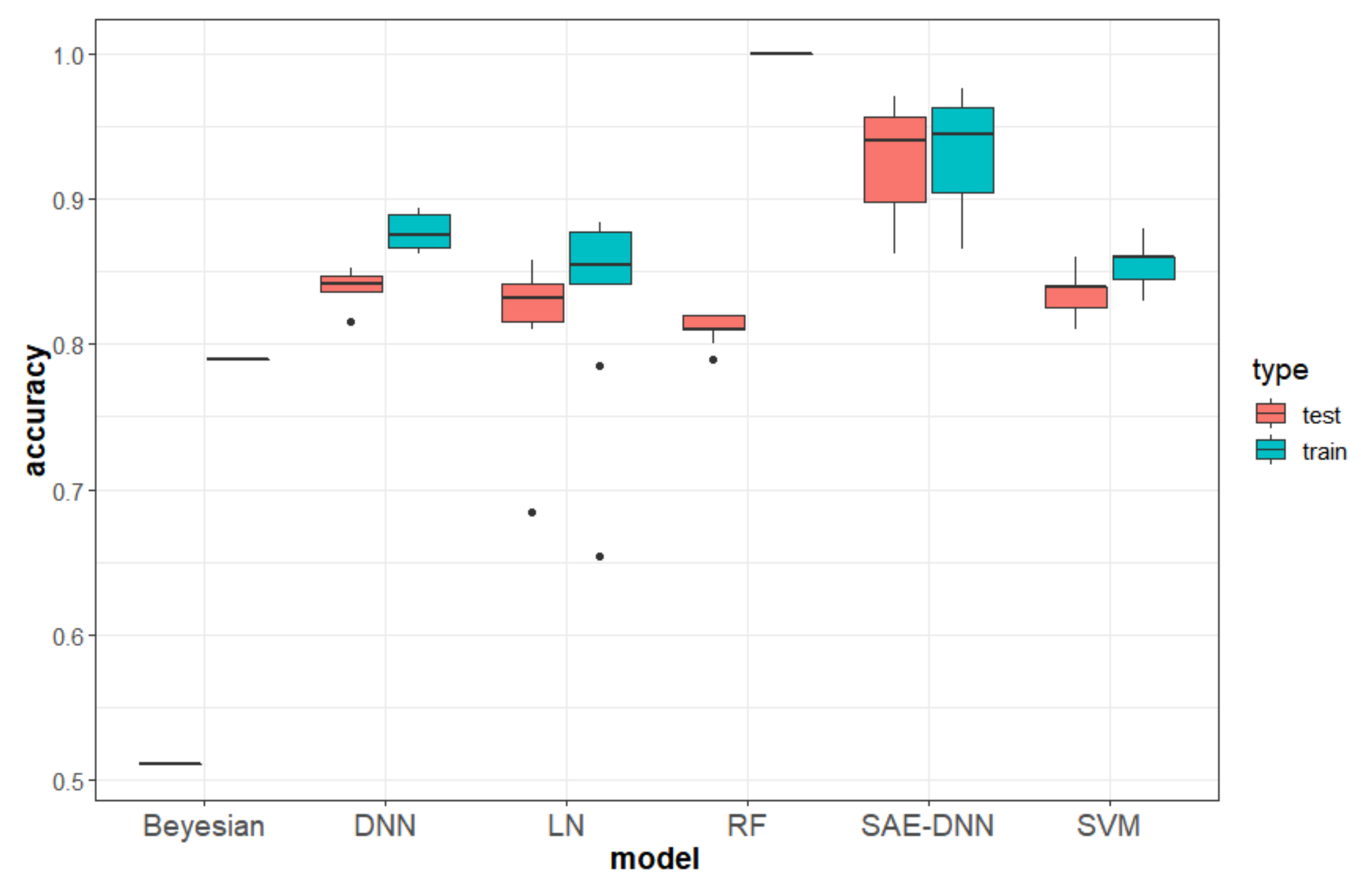
Comparison with baseline: We compared the results of baseline methods: Naive Bayes, Random Forest (RF, ntree = 100, mtry = 3), linear regression, Support Vector Machine (SVM, kernel = radial), deep neural networks (DNN, hidden units (200, 400, 400, 200), and SAE-DNN (hidden units (200, 400, 400, 200) (Figure 14). We found an overfitting about decision trees and Bayesian, which cause the test set accuracy to only be about 50%, while other models performed well on both the training and test sets. SAE-DNN’s performance is the best one. The training set accuracy can reach 95.7%, and the test set accuracy can also reach 93.5%.

Comparison of different hyperparameter: We further analyze the impact of hyperparameters in the framework, including the structure of SAE-DNNs. In the following discussion, we change one hyperparameter while keeping other hyperparameters unchanged.

Table 9. Comparison of the structure of SAEDNNs.

Hidden Layers	Hidden Units	$\mathit{L}\mathit{o}\mathit{g}\mathit{L}\mathit{o}\mathit{s}\mathit{s}$	$\mathit{A}\mathit{C}\mathit{C}$
3	(100,100,100)	0.411	0.827
3	(200,200,200)	0.402	0.849
3	(400,400,400)	0.345	0.903
4	(100,100,100,100)	0.313	0.906
4	(100,200,200,100)	0.288	0.912
4	(200,200,200,200)	0.274	0.924
4	(200,400,400,200)	0.253	0.935
5	(400,400,400,400)	0.269	0.922
5	(400,800,800,400)	0.277	0.92

shows the performance of different SAE-DNNs structures, the structure of four hidden layers and (200,400,400,200) hidden units perform best.

Comparison with other researches:

Table 10. Comparison with other researches.

Research	Data	Problem	Results
Du et al. [8]	AFC records in Beijing	Detecting Pickpocket Suspects	Recall = 0.931
Zhao et al. [7]	AFC records in Beijing	Detecting Pickpocketing Gangs	Recall = 0.94
Tang et al. [40]	AFC records in Shenzhen	Detecting Passenger Flow Anomalies	F1 = 0.87
Chong et al. [41]	PTS records and tweets in USA	Detecting Flow Anomalies	RMSE lower than baselines
Silva et al. [42]	GPS in unmentioned country	Anomaly Detection in Roads	Algorithms scores = 0.87
Proposed method	AFC records in Beijing	Anomaly Detection in subway	Accuracy = 0.935

PTS denotes to Public Transportation System.

shows the comparison with other researches. Tang et al., Chong et al. and Silva et al. [40,41,42] aimed to detect Flow Anomalies in public transportation or road transportation; our proposed method performs better than these methods. In addition, Zhao et al. and Du et al. [7,8] aimed to detect pickpocket by AFC data, and our proposed method could not only identify pickpocket, but also could identify beggars etc., which reaches a similar result with state of the art.

7.3. Discussion

Between inbound and outbound stations, the passenger could, in theory, travel through multiple paths, and if there was a problem like a train stopped, travelers were asked to take alternative routes. Although this situation will not happen too frequently, we should pay attention to it. Chilipirea, et al. [43] developed three algorithms for determining stops and movements for GPS-based datasets and explored their applicability to WiFi-based data, if the problem of train stops etc. are considered in our research, it will reduce the false positive phenomenon of the model.

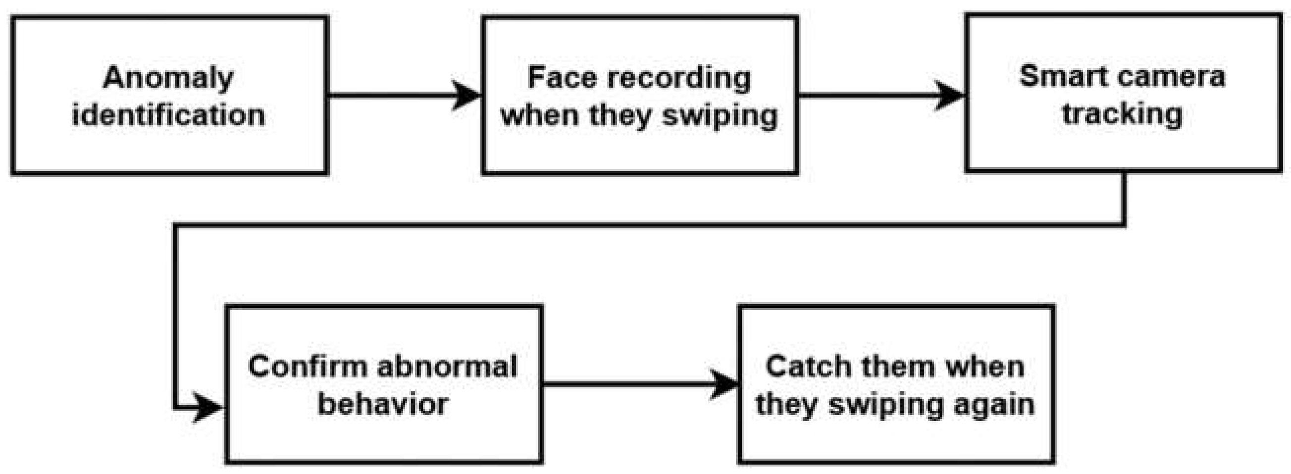
In addition, our research team is developing a system that addresses the suspected behavior (Figure 15). The system can capture the faces of passengers with suspected behavior when they swipe their cards and applies a smart camera to continuously record the behaviors of these passengers. Once the suspected behavior is confirmed, the subway staff can catch the offending passengers the next time that they swipe their cards. In order to protect privacy, normal card swiping will not be recorded.

8. Conclusions

This paper proposes a method for identifying the LSSS in the subway based on the shortest path and analyzes its travel mode. In combination with the past research of scholars, we try to quantify the suspected behavior with a database of assumed suspected behavior records. Finally, we extract the spatial-temporal travel features of passengers, and we propose a SAE-DNN algorithm to identify suspected anomalie; the accuracy of the training set can reach 95.7%, and the accuracy of the test set can also reach 93.5%, which provides a reference for the subway operators and the public security system.

Besides, three issues need to be focused on:

Dataset: It is hard for us to get real-world labels. Indeed, the suspected passengers are not real thieves, etc. the labels of the suspected abnormal passengers were marked manually based on the high similarity. This is a result judged by the rail transit safety experts and police based on data and experience. Using such a dataset is because they show some odd rides exactly. Our model performs well in identifying assumed abnormal behaviors, this means that if the real-world dataset is obtained, the model has great potential to be effective.

Method: Since we focus on the extraction and analysis of spatial-temporal features, this paper is inadequate regarding the model construction of LSSS identification. We only rely on the shortest path algorithm and do not consider the diversified path selection problem of passengers. We establish a constant transfer time and do not consider the difference in the spatial structure of different stations. For this reason, we deliberately set this constant to the maximum value of all transfer times and try to avoid defining normal passenger flow as abnormal. However, this approach may miss some abnormal passenger flow. In future research, we can infer the passenger’s path selection problem based on probability and achieve a more accurate identification model of suspected abnormal passenger flow.

Privacy: Firstly, the smart card data we collect is anonymous, the cards do not involve any personal information. So, the privacy of passengers was not be touched in the model. Secondly, if the system is applied to the real world, the offence to regular passengers caused by the error of classification is a key problem. Improving the performance of the model can reduce such risks; and using surveillance video to verify the behavior can fundamentally solve this problem. In addition, surveillance video Intelligent verification without artificial observation is a good future work.

Others: We are not sure that LSSS is commonly found in other underground systems all over the world, but we believe that odd rides are commonly found all over the world; for example, there are thieves everywhere, and their habits must be different from those of ordinary passengers; LSSS is just one of the odd rides, and we chose it for our research. The proposed framework of research methods can quantify these odd riding behaviors and identify them, this is the value that this paper brings to the whole world.