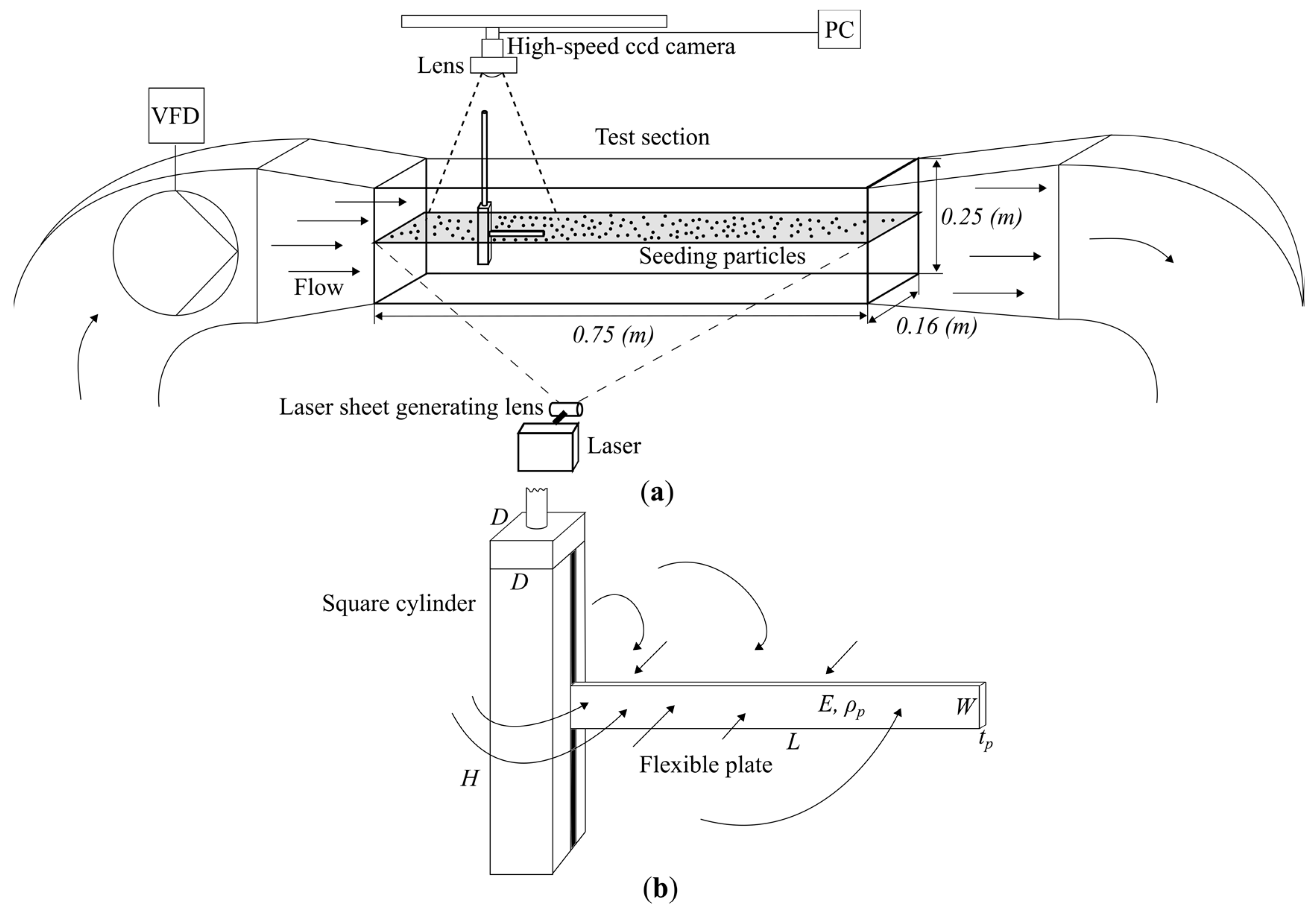
Article

Flexible Plate in the Wake of a Square Cylinder for Piezoelectric Energy Harvesting—Parametric Study Using Fluid–Structure Interaction Modeling

by
Emmanuel Mbondo Binyet
,
Jen-Yuan Chang
* and
Chih-Yung Huang
Department of Power Mechanical Engineering, National Tsing Hua University, Hsinchu 30013, Taiwan
*
Author to whom correspondence should be addressed.
Energies 2020, 13(10), 2645; https://doi.org/10.3390/en13102645
Submission received: 2 May 2020 / Revised: 18 May 2020 / Accepted: 19 May 2020 / Published: 22 May 2020
(This article belongs to the Section A: Sustainable Energy)

Abstract

:
Piezoelectric energy harvesters can scavenge energy from their ambient environment in order to power low-consumption electronic devices. The last two decades have seen a growing interest towards vortex-induced vibration harvesters; most harvesters consist in rigid splitter plates oscillating at higher frequencies. The concept presented here is a low-frequency undulating flexible plate placed in the wake of a square cylinder. Piezoelectric patches can be placed at the plate surface to harvest the strain energy arising when the plate bends. The flapping pattern mimics an anguilliform swimming motion. There is a great need to establish correlation between wake generating bluff body size, plate dimensions and power output. Geometric parameters were investigated using water tunnel experiments, particle image velocimetry and fluid–structure interaction modeling. Results showed that for a given plate length and within a given freestream velocity range, there is a square cylinder diameter and a thickness that optimize the plate–wake interaction. Longer plates yield greater power output but have lower flapping frequencies. Additionally, the more frequent curvature changes occurring can result in charge cancellation among the piezoelectric cells. Consequently, the estimated conversion efficiency from mechanical strain to electricity is higher for shorter plates.

1. Introduction

Square cylinders placed in fluid flow generate an oscillatory wake behind them; the impinging flow detaches at the front edges and rolls up into vortices that are shed alternatively in the wake. This phenomenon is known as the Karman vortex street and is characterized by a travelling pressure wave. Flexible plates placed in such an oscillatory wake would undergo periodic oscillations that could generate electricity through piezoelectricity. Piezoelectric energy harvesters have a growing potential for powering remote sensors and low-consumption electronic devices, especially where battery replacement is not a convenient task. Besides, batteries put great stress on the environment at the end of their life cycle and therefore it is important to find sustainable alternatives. Various vortex-induced vibrations piezoelectric harvester designs have been presented in the last two decades owing to the rise in the popularity of piezoelectric materials. While An et al. [1] make use of a pivoting rigid plate in the wake of a cylinder to squeeze adjacent piezoelectric patches near the hinged end, most harvesters consist in fluttering rigid splitter plates with piezoelectric patches mostly near the clamped end. Tang et al. [2] developed an aero-electromechanical model validated by wind tunnel experiments for energy harvesting fluttering cantilever plates. Their harvester is a rigid plate placed in the wake of a square cylinder that hosts piezoelectric cells on its surface. According to the power output measurements, most of the power came from the cells placed from the clamped end to within 40% of the total length while the cells near the free end of the cantilever plate recorded negligible power output because of the low curvature. In the prototype developed by Akaydin et al. [3], the cylinder is attached to the free end of the aluminum plate while the fluid flow goes from the free end side towards the clamped end side. PZT (lead zirconate titanate) patches are located near the clamped end. They performed wind tunnel tests and measured the strain at the patches’ location and successfully modeled the effect of load resistance on the natural frequency and damping ratio. They recorded an overall aero-electromechanical efficiency of 0.72% and an electromechanical efficiency of 26%. The plate was mostly oscillating in the two first bending modes; the dynamic coupling was strong and electromechanical coupling weak. To illustrate the electromechanical coupling, Erturk and Inman [4] showed in their experiments with a PZT-5H (highest piezoelectric constant lead zirconate titanate) bimorph cantilever without a tip mass a delay of around 4% in the first mode natural frequency between short circuit R l = 0 and open circuit R l = 1000   ( k Ω ) . Vibration amplitude also increased with the resistive load. According to Shafer and Garcia [5], at most 44% of the strain energy can be converted to electrical energy. Tang et al. [2] found maximum conversion efficiencies nearing 60%. The conversion efficiency depends on the load resistance and the frequency; this is why different studies achieved different values. According to Shu and Lien [6], considering rectification of the current, the conversion efficiency can range from 20% to close to 90%. When converting stress into electric charges, piezoceramics have higher piezoelectric constants than piezoelectric elastomers. On the other hand, their rigidity makes them unfit for acute bending applications. Following the growing interest towards piezoelectricity, composite piezoelectric materials combining both flexibility and high piezoelectric constants are being developed. Some of those piezocomposite energy harvesters (PCEHs) consist in hard piezoelectric particles within an elastomer. The main challenge encountered is the inefficient stress-transfer within the soft matrix. Zhang et al. [7] proposed a piezoceramic skeleton inspired by a sea porifera filled by a soft polymer matrix. Such a structure significantly enhances the energy harvesting performance of the piezocomposite by effectively distributing the stress while maintaining elasticity. They measured a power output about 16 times higher than for conventional PCEH devices. Han et al. [8] developed a flexible piezoelectric membrane using a thin film of PZT adhering on a polymer membrane for use in self-powered acoustic sensors. These state-of-the-art piezoelectric materials could be implemented in energy harvester concepts in order to further increase the conversion efficiency.
Most concepts that have been investigated rely mostly on small to moderately large deflections. Less literature is available on piezoelectric harvesters relying on large-amplitude flexural vibrations. As a reason, we turned our interest towards flexible undulating ribbons with piezoelectric patches along the plate’s surface [9,10,11,12,13,14,15]. The subject of the present research is based on the “energy harvesting eel”. This concept was first introduced by Taylor et al. [9], which recalls the anguilliform swimming motion. This mode of fish locomotion is mainly two-dimensional, allowing the fish to spend less energy and cover longer distances [16]. The prototype of Taylor et al. [9] consists in a bluff body hosting in its wake a polymeric flexible neutral layer with on each side: piezoelectric cells composed of PVDF segments sandwiched between electrodes and a sealing layer. Aiming to maximize the strain within the cells, several water tunnel studies have described the influence of the bluff body size as well as the width and length of the plate. Allen et al. [10] tested a prototype with a gap between the bluff body and the clamped end, they carried out water tunnel experiments with two different bluff body widths and two different length-to-width ratios of the plates and gave a thorough description of the plate dynamics. Shi et al. [11,12] tested two different plate lengths and found that longer plates yield more strain energy due to an earlier transition to a travelling wave flapping pattern. Taylor et al. [9] used the mode shapes of a free-vibrating cantilever beam to describe the dynamics of their “eel”. This approach which was used by Binyet et al. [13,14,15] to investigate the plate length influence on the strain energy. Those studies did not provide optimum geometric parameters of the bluff body and plate for maximum strain energy generation. Moreover, no design information is available on plate thickness, which is a tremendously important parameter regarding plate response. The dynamic pressure impinging on the plate triggers its response and the response will in turn influence the dynamic pressure distribution [17] as the flow around the plate is now modified by the plate motion. For this reason, the bluff body size, the plate length and its stiffness are the main parameters dictating the response. Binyet et al. [13] attempted to fill the gap in a preliminary study, but the data was not exhaustive and the superimposed layers approach to increase the thickness does not represent the increase in stiffness accurately. While rigid-splitter-plate-oscillation-based harvesters can be modelled mathematically with great accuracy, undulating-plate-forced motion within a turbulent wake is dominated by large-amplitude undulations resulting in a complex fluid–structure interaction mechanism [9,10,11,12,13,14,15]. For this reason, the response can be investigated either by carrying out water (wind) tunnel experiments or through fluid–structure interaction modelling coupling both computational fluid dynamics and computational structure dynamics.
Simulations are a great tool to carry out parametric studies as they spare costly experiments. However, fluid–structure interaction (FSI) modelling of unstable structures at practical Reynolds numbers remains a difficult task. The FSI model has to be validated through comparison with experimental data or existing benchmarks. Turek et al. [18] developed a 2D benchmark in the case of flow around a cantilever plate clamped to a cylinder under incoming laminar flow. The benchmark results give the lift and drag on the cylinder as well as the displacement and oscillating frequency of the cantilever plate. The accuracy of the different FSI modelling approaches can be tested against their benchmark results. Giannelis and Vio [19] carried out the Turek et al. FSI2 benchmark (large deformation, periodical oscillations) coupling ANSYS Mechanical and ANSYS Fluent, using a structured O-grid of hexahedral elements, a laminar-pressure-based solver, second-order pressure and a second-order upwind momentum specification. Under-relaxation of the pressure data transfer from the fluid as well as mesh diffusion were specified to avoid mesh distortion. Their results showed excellent agreement with the benchmark with error in the quantities of interest below 6%. The FSI3 (large deformations and complex oscillations) benchmark of Turek et al. is available in the COMSOL application gallery [20]. Results show good agreement, with 2% error in the mean drag, 25% error in the mean displacement, y, and 7% error in the amplitude. COMSOL Multiphysics is a commercial software that can solve fluid–structure interaction problems. It uses a finite element approach to discretize the governing equations. The fluid and solid domains are resolved using one single solver. A large coefficient matrix accounting for all the degrees of freedom makes it possible to solve the system in a fully coupled manner. The fluid–structure interface and mesh motion is described using the Arbitrary Lagrangian–Eulerian (ALE) method. A Lagrangian frame is used to describe the solid domain while an Eulerian frame is used for the fluid domain. The Arbitrary Lagrangian–Eulerian method allows for the inner grid points to be moved independently of the fluid motion. This can prevent mesh distortion. However, at the interface, the kinematic condition (continuity of velocities) is enforced so that the fluid and structural domain do not overlap or detach. At the interface, the structural nodes and fluid nodes are superimposed [21]. Curatolo et al. [22] used COMSOL’s fluid–structure interaction, electrostatics and electric circuit packages all together in order to estimate the electrical energy output of a deformable piezoelectric solid in water flow. The concept under investigation is similar to that of Akaydin et al. [3]. Fluid flow is impinging on a concave half-tube connected to the free end as the clamped end is connected to a fixed cylinder. The piezoelectric layer is connected to the clamped end. Their model has about 3 · 10 5 degrees of freedom. The amplitude of the free end was around 50 mm, but the piezoelectric layer oscillates with small amplitude. They computed an average power of 0.5 mW/m in the PZT 5-A (lower piezoelectric constant lead zirconate titanate) layer under an incoming velocity of 1 m/s. Load resistance influence as well as electromechanical coupling were not investigated. Because most of the studies in the literature are only concerned with incoming laminar flow, to fill the gap, De Nayer et al. [23] realized an FSI benchmark for a 2 mm thick flexible rubber plate clamped to a cylinder in turbulent flow (Reynolds number of 30,470). They carried out water channel experiments in order to measure the plate displacement, flapping frequency and Strouhal number in order to validate their FSI simulations. They also used particle image velocimetry to capture the flow field, but no detailed analysis of the wake flow pattern was made. Their FSI model is based on a partitioned coupling scheme: the fluid flow is predicted by the large-eddy simulation technique and the structure response is computed by solving the momentum equation in a Lagrangian frame of reference. The solution is obtained through implicit coupling between the computation of the pressure and the structural displacements. The flapping frequency was very well predicted (relative error of around 2%). However, the overprediction of the amplitude mostly exceeded 10%. The velocity magnitude was overpredicted in the acceleration zone around the cylinder (under 20%), but the flow structures were all in agreement with the PIV recordings. The commercial software ANSYS Fluent is based on the finite volume method, which is the most common approach as it is closer to the physics of fluid flow. The discrete algebraic equations are expressed following exactly the conservation law. Moreover, after decades of software development, techniques have been embedded for solution stabilization. Molina-Aiz et al. [24] agreed with several previous comparative studies and concluded that the finite element method was computationally less efficient than the finite volume method for solving fluid flow.
The present study aims to provide information on the bluff body size and plate thickness that maximize the power output by carrying out fluid–structure interaction modelling of the undulating plate coupling the commercial solvers ANSYS Fluent and ANSYS Mechanical from Ansys Inc. (Canonsburg, PA, USA) version 14.5. To our knowledge, in most FSI-modeling-related studies, the plate-deflected shapes are limited to the first two cantilever beam bending modes. Whereas, in the present study, large-amplitude deflected shapes up to the first four bending modes are modelled. Water tunnel experiments were performed in order to assess the accuracy of the model, describe the flow and flapping pattern and finally evaluate the power generated by bending. In conclusion, optimum thickness and square cylinder diameter vary with plate length and incoming flow velocity. Design information was provided for several free-stream incoming velocities. In general, longer plates yield greater power output but have lower piezoelectric conversion efficiencies.

2. Experimental and Computational Methods

2.1. Water Tunnel Experiments: Particle Image Velocimetry and Plate Deflection Analysis

Experiments were carried out in a recirculating water tunnel (schematic shown in Figure 1a); the freestream velocity in the test section was adjusted using a variable frequency drive (VFD) controlling a pump. The velocity was varied from around 0.6 m/s to around 1 m/s, giving a Reynolds number based on the square cylinder of around 9200 to 14,300 and vortex shedding frequencies of around 6 to 9 Hz. The square cylinder vortex shedding frequencies f v are calculated from
f v = S t · u f D ,
where St = 0.14 represents the Strouhal number for a square cylinder (Okajima) [25]. The Reynolds number is expressed as
R E = ρ f · u f · D μ f ,
where D represents the square cylinder diameter, ρ f the density, u f the incoming fluid velocity, and μ f the dynamic viscosity of the fluid. The kinematic viscosity is ν f = μ f ρ f ; values are given in Table 1.
The diameter of the square cylinder was of D = 15 mm; its height was H = 105 mm (schematic shown in Figure 1b). Compared to the cross-sectional area of the test section, the blockage was under 5%. Although turbulence is always a tridimensional phenomenon, for slender cylinders, the wake can be assumed to be quasi-two-dimensional far from its top and bottom surfaces. The present study relies on the core assumption that the plate motion is quasi-two-dimensional, as it is more efficient for converting the impinging flow into harvestable strain energy. For this reason, the plate width was kept under a value of W = 10 mm so that torsion was not significant. Piezoelectric materials were not used during this investigation, but, instead, the plate was made of polyethylene terephthalate (PET), which shows similar density and stiffness to piezoelectric PVDF. Consequently, it can presumably mimic the piezoelectric material behavior. The properties of the PET-based plates used are listed in Table 2. A prior measurement campaign that focused only on the plate deflection was run using a 500 frame-per-second high-speed camera. It was then followed up with a second measurement campaign focusing on plate deflection and the related flow field, which was run with a 5000 frame-per-second high-speed camera. The thickness of the plates used among the measurement campaigns was of 80, 100 and 120 microns. The square cylinder was made of one aluminum block connected to a fixation rod and of two aluminum blocks screwed together while clamping the plate in between them. Tape was wrapped around the square cylinder to seal the gap where the two blocks unite. A 532 nm 3 watts green laser pointing into a cylindrical lens generated a bright laser sheet illuminating the plate and the flow field. PVC spheres of a diameter of 3 µm acting as seeding particles were poured in the test section to scatter the light from the laser sheet. The particles have a density which is close to water to ensure that the fluid motion is well represented by their displacement. Particles appear bigger than their actual size on the images captured because they scatter the light in all directions. The flow field around the plate as well as the plate deflection were captured by the high-speed camera. The frames were stored on a computer for further image processing. From the frames, the flow field was computed using the particle image velocimetry (PIV) method and the plate deflection was deduced by measuring the plate position. PIV consists in measuring the displacement of the identical seeding particles between each pair of frames; the velocity vectors can be deduced from the displacement vectors and the elapsed time between the pair of frames. The foundation of PIV is discrete cross-correlation: the successive images pairs are divided into interrogation areas Ai and Bi; the discrete cross-correlation function measures the agreement for a given displacement vector for each area pair ABi. The discrete cross-correlation function [26] is expressed as
C ( m , n ) = i j A ( i , j ) B ( i m , j n )
where m and n account for the pixel offset between interrogation areas A and B .
The function yields an intensity peak for identical particles in the first and second exposure which are the i = j terms; on the opposite, a noise floor results from the i j terms which are random particles. The coordinates of the peak in the correlation matrix plane give the most probable displacement vector of the seeding particles from Ai to Bi. The u and v components of the velocity vector can then be retrieved knowing the time lapse between both exposures. The software PIVlab developed by Thielicke [26] was used for computing the velocity vectors of the characteristic deflected shapes. The PIV routine consists in first selecting the region of interest and masking the plate, then applying contrast-limited adaptive histogram equalization (CLAHE), high-pass filtering and a Wiener 2 denoise filter to optimize the image before executing the frequency domain cross-correlation algorithm. Three passes were carried out with window sizes of 64, 48 and 32 pixels. It was not possible to reach 16 pixels because of the camera resolution, and mostly because the full plate is required to be present in the frame. Because the displacement of the particles between frames has to be kept below 16 pixels, a frame rate of 5000 fps was necessary. An in-house Matlab code was developed for shape capture; the frames are first cropped at the clamped edge, converted to grayscale and finally to negative. The frames are then filtered, so that the plate is emphasized and the particles diminished. The negative image is converted to a binary image according to a suitable threshold level; this makes the plate and the particles appear in white (pixels with a 1 value) while the background is in black (pixels with a 0 value). The particles are then removed by running a loop that turns isolated 1-valued pixels to 0-valued pixels in the matrix columns. Isolated pixels are mostly surrounded with 0-valued pixels or are out of plate reach. Finally, the plate deflection is determined by locating in each column the next group of 1-valued pixels either above or below the neutral line. The distance from the neutral line to each group of pixels at each horizontal position gives the vertical coordinate of the plate w. From the w coordinate of the plate, each corresponding x coordinate is determined applying the Pythagorean theorem, as for each vertical position increment there is a corresponding horizontal shift because the neutral line is inextensible. The measured positions are converted from pixels to millimeters through a calibration image. The raw deflection data are finally fitted with a n-degree polynomial that is the best fit in the least-squares sense.

2.2. Plate Response

From the plate deflection data for each frame, the strain energy and modal contribution are computed. All the following computations rest on several fundamental hypotheses. The plate motion can be regarded as two-dimensional with no torsion, no shear deformation, no warping, nor any deformation along the plate width. Moreover, the neutral line is assumed inextensible as stated by Lighthill [16]; in other words, there is no tension at the centerline. It is also assumed that the swelling or contracting of the plate under compression or traction is negligible (no deformation along the thickness). Therefore, the plain sections remain plain and perpendicular to the neutral line and the cross-sections remain the same. These assumptions make complete sense when the flexible plate is related to the anguilliform swimming motion.

2.2.1. Strain Energy

Resulting from the above hypotheses, Hooke’s law linking longitudinal strain to longitudinal stress is written as ε x = σ x E . The longitudinal strain in pure bending is expressed as ε = y ρ i where ρ i is the radius of curvature. Obviously, the smaller the radius of curvature, the greater the strain, from trigonometry and by means of Hooke’s law. The tensile stress within the beam is given by
σ i = y i E w ( 1 + ( w ) 2 ) 3 2 .
Equation (4) is used by Frisch-Fay [27] for analyzing large deflection of flexible rods. It is considered valid even in the case of large deformations under the aforementioned assumptions. The derivative terms are approximated with finite differences:
w ( t i ) = w x w ( t i , i ) w ( t i , i 1 ) x ( t i , i ) x ( t i , i 1 ) ; w ( t i ) = 2 w x 2 w ( t i , i + 1 ) 2 w ( t i , i ) + w ( t i , i 1 ) ( x ( t i , i ) x ( t i , i 1 ) ) 2 .
The strain energy is the work done by the stress extending the plate of width W, expressed as
U = 1 2 W E t p 3 12 0 L 0 ( w ( 1 + ( w ) 2 ) 3 2 ) 2 d x ,
The integral is computed numerically using the composite trapezoidal rule for each frame at time t i . The most important index to compare the different plates’ harvesting capabilities is the bending power; it is defined as the rate of change of strain energy. The instantaneous bending power is defined as
P t i = d U d t U t i + 1 U t i 1 2 Δ t .
Then, the time-averaged bending power is defined as P s = 1 T 0 T P t i d t , where T is the average time interval, which is mainly the sample size. For comparison with the two-dimensional FSI model, the results are expressed in terms of average bending power per width: P s W = P s W .

2.2.2. Modal Analysis

From observation of the plate’s deflected shapes, it appears that the mode shapes of a clamped-free cantilever beam under free vibration (shown in Figure 2b) can be used to describe the complex bending pattern of the plate. Indeed, each bent shape can be represented as a combination of those basic mode shapes. Although the mode shape expressions are derived from the small-deformation theory, they can still be used as a marker of the level of the bending occurring when describing the bending pattern. The deflected shapes of the clamped-free cantilever beam vibrating in the mode m (eigenfunction) are expressed according to Sonalla [28] as
X m ( x ) = ( cosh α m x cos α m x ) γ m ( sinh α m x sin α m x ) ,
Consequently, the natural frequency of each mode is defined as
f m = 1 2 π α m 2 E I ρ p A ,
where α m represents the eigenvalues: α m · L 1.88 ; 4.69 ; 7.85 ; 11 . γ m 0.73 ;   1.02 ;   1 ;   1 are the corresponding eigenvectors. A = W · t p represents the cross-sectional area of the plate. I = W p t p 3 12 accounts for the second moment of inertia. Thinner, slender, longer plates have lower natural frequencies and thus are more likely to have deflected shapes resembling the higher-order mode shapes. Calculating the contributions from each mode shape within the measured deflected shapes indicates the complexity of the bending pattern for each shape. From the deflection data w i and Δ x i = x i x i 1 , the modal contributions for each mode m are estimated according to
B m = i = 1 n w i · X m i · Δ x i = 1 n X m i 2 · Δ x .

2.2.3. Piezoelectric Energy Harvesting

Piezoelectric PVDF generates a voltage when a force is applied to it because of the resulting charge concentration on each side of the layer generated by the strain (traction or compression) within the material. Considering a cantilever beam with one neutral layer and one piezoelectric layer on each side as shown in Figure 3a, the electric displacement D 3 is related to the stress and the electric field according to [4,29]:
D 3 = d 31 · σ x ( y ) + ε p σ · E 3 ,
where d 31 is the piezoelectric stain constant in 31 mode (Table 3), ε p σ the electric permittivity of the piezoelectric layers under constant strain and plain stress and E 3 the electric field.
The voltage across the electrodes of each layer is V l ( t ) . Considering a parallel connection of the electrodes, the instantaneous electric fields for the active layers B and A are
E 3 ( t ) = V l ( t ) t l   and   E 3 ( t ) = V l ( t ) t l .
The electric current through the electrodes is given by the Gauss law integrating over the piezoelectric layer area, where L l is the length of the piezoelectric layer and W l its width [4]:
d dt ( A D · n d A ) = V l ( t ) R l ,
where D is the vector of electric displacement, n is the unit outward normal. In this case, the only component of D which matters is D 3 since n is along the thickness (3-axis). R l is the load resistance. Substituting Equations (4), (11) and (12) into Equation (13) yields
d dt ( 0 L l 0 W l D 3 d x d z ) = V l ( t ) R l .
Hence, for layer A:
d dt ( E l d 31 W l 0 L l y ( x , t ) w ( 1 + ( w ) 2 ) 3 2 d x ε p σ · V l ( t ) t l L l W l ) = V l ( t ) R l ,
y ( x , t ) can be taken as the distance between the neutral axis and the center of the piezoelectric layer, assuming that the neutral layer at the center has a thickness t p : y l = ( t l + t p ) / 2 . Now assuming that t p = t l , a differential equation for the voltage V l ( t ) is obtained for layer A:
E l d 31 W l t l d d t ( 0 L l w ( 1 + ( w ) 2 ) 3 2 d x ) + ε p σ L l W l t l · d d t ( V l ( t ) ) + V l ( t ) R l = 0 .
After integrating in time assuming that Δ t is small and rearranging, the expression for the voltage at time t + Δ t can be determined for a given load resistance value R l by setting an initial value V l t :
V l t + Δ t = R l ( 1 + ε p σ L l W l t l R l Δ t ) Δ t ( E l d 31 W l t l ( 0 L l w ( 1 + ( w ) 2 ) 3 2 d x ) | t t + Δ t + ε p σ L l W l t l · ( V l t ) ) ,
and the resulting power output is P l = V l ( t ) 2 R l .
The integral of the curvature in Equation (17) is computed numerically using the composite trapezoidal rule together with finite difference approximation from the deflection data. There is an optimum resistive load value which gives the maximum power output for a given frequency. On the other hand, it is fundamental to keep in mind that the plate response w ( x , t ) also depends on the load resistance R l due to mechanical damping. When R l is close to zero, the damping is null and increases with the resistive load. However, for the present study, it can be assumed that electromechanical-coupling-induced stiffness increase brought by the load resistance is negligible (in the order of several percent for the cantilever piezoelectric bimorph of Azizi et al. [30]). This assumption makes sense considering the strong dynamic coupling in place as the plate motion mostly follows the vortex shedding frequency. Under weak electromechanical coupling, the electrical energy being harvested has no influence on the response and therefore, stiffening can be neglected.

2.3. Fluid–Structure Interaction Modelling

2.3.1. Computational Fluid Dynamics

Governing Equations

The flow has to be modelled with a compressible fluid because constant density fluids yield an infinite wave speed c = ( P ρ ) . An incompressible fluid yields larger pressure gradients than a compressible fluid for a similar displacement of the solid interface. For this reason, when using water as a fluid medium, unphysical pressure spikes occur during the solution process leading to great stress applied to the solid interface, resulting in even greater displacements of the structure. In this case, the mesh cells become so distorted that the vertices are distributed, such that the bounding faces intersect each other and the vertices penetrate opposite faces. Those are referred as “negative cell volumes”. When they occur, divergence of the calculation is the only outcome. For simplicity, the fluid medium was changed to compressible air, and, consequently, the velocity at the inlet was changed according to the Reynolds law of similitude. Switching the fluid medium to air yields increased flow velocities and, therefore, increased vortex shedding frequencies followed by greater flapping frequencies. Air has a kinematic viscosity around 15 times that of water, meaning it is 15 times more diffusive. The fluid kinematic viscosity also describes how vorticity diffuses through a fluid and, therefore, using air instead of water would yield different vorticity fields in the far wake.
Because the fluid is compressible, density weighted time averaging [31] is required to model the turbulent flow. The continuity equation is expressed as
ρ ¯ t + x i ( ρ ¯ u i ˜ ) = 0 ,
The momentum equation, also called the Favre-averaged Navier–Stokes equation, is expressed as
t ( ρ ¯ u ˜ i ) + x j ( ρ ¯ u ˜ i u ˜ j ) = ρ ¯ g i p ¯ x i + x j μ [ ( u ¯ i x j + u ¯ j x i ) 2 3 u ¯ k x k δ i j ] + x j ( ρ u l u J ¯ ) ,
where ρ stands for the density of the fluid, the u i ˜ terms represent the time-averaged velocities, p ¯ the time-averaged pressure and δ i j the kronecker delta. The terms on the left-hand side are the local rate of change of momentum and its advection. The terms on the right-hand side are the gravity action, the pressure gradient, the viscous stresses, viscous dissipation and expansion or compression, and finally the term ρ u l u J ¯ called Reynolds stress. This term cannot be resolved and needs to be modelled in order to close the momentum equation. The Renoylds stresses are related to the mean velocity gradients according to the Boussinesq hypothesis [32]:
ρ u l u J ¯ = μ t ( u ¯ i x j + u ¯ j x i ) 2 3 ( ρ ¯ k + μ t u ¯ k x k ) δ i j ,
where μ t represents the turbulent viscosity, which is assumed to be an isotropic scalar quantity. Hence, the turbulence is assumed to be isotropic meaning that the normal stresses are equal: ( u ) 2 ¯ = ( v ) 2 ¯ . Considering the plate motion to be mostly two-dimensional where out-of-plane bending and torsion are neglected, the assumption is valid. The turbulence model chosen is the realizable k ε model. It is still accurate for flows involving vortices and rotation, separation and recirculation while being less computationally intensive than the Reynolds stress model. k is the turbulence kinetic energy defined as half the trace of the Reynolds stress tensor: k = 1 2 ( u l u l ˜ ) and ε 2 ν S l J S l J ¯ its dissipation rate. In the realizable k ε model, the modeled transport equations for k and ε are
t ( ρ ¯ k ) + x j ( ρ ¯ k u ˜ j ) = x j [ ( μ + μ t σ k ) k x j ] + G k ρ ε ,
t ( ρ ¯ ε ) + x j ( ρ ¯ ε u ˜ j ) = x j [ ( μ + μ t σ ε ) ε x j ] + ρ C 1 S ε ρ C 2 ε 2 k + ν ε ,
where C 1 = m a x [ 0.43 , η η + 5 ] , η = S k ε , where S is the modulus of the mean rate of strain tensor defined as S 2 S ˜ i j S ˜ i j , where, for variable density flows, the rate of strain tensor is defined as S ˜ i j = ( u ˜ j x i + u ˜ i x j 1 3 u ˜ k x k δ i j ) . G k = ρ u l u J ¯ u ˜ j x i represents the production of turbulence kinetic energy which is approximated according to the Boussinesq hypothesis: G k = μ t S 2 . The production of turbulent kinetic energy is the result of the Reynolds shear stress and the velocity gradients. The vorticity and the rate of strain also result from those velocity gradients. The kinetic energy lost due to the shearing of the mean flow is gained by the turbulent fluctuations and then dissipated. The turbulent viscosity or eddy viscosity is computed from μ t = ρ C μ k 2 ε , where C μ is computed from the model constants, the strain rate, the rotation rate, k and ε .
The energy equation has to be solved together with the equation of state linking the thermodynamic quantities together. This is for further use in the momentum and continuity equations as the density varies due to pressure and temperature changes. Assuming a perfect gas, the equation of state linking the thermodynamic pressure p to the temperature T is p = ρ R T , where R = stands for the perfect gas constant. The conservation of energy of the particle is written as
t ( ρ E ) + · ( V ( ρ E + p ) ) = · ( k e f f T + τ = e f f · V ) .
The two terms on the right-hand side of Equation (23) represent the heat conducted through the faces of the control volume and dissipated by viscosity. k e f f represents the effective conductivity. τ = e f f is the viscous stress tensor. The total energy of the particle which varies with the action of the gravitational forces, the velocity, the pressure, the viscosity and the heat transfer is E = h p ρ + | V | 2 2 . The enthalpy per mass is calculated as h = T r e f T c p ( T ) d T , where c p ( T ) is the specific heat and T r e f the reference temperature.
All the above governing equations can be rewritten in the general transport equation form [33,34]:
ρ ϕ t + · ρ U ϕ = · ( Γ ϕ ) + S ϕ .
After rearranging the governing equations and setting appropriate diffusion coefficients Γ and related source terms S ϕ , the general variable ϕ can be set as 1 to obtain the continuity equation, as u ˜ i to obtain the momentum equation and so forth for all the governing equations.

Solution Method

The finite volume method consists in integrating the transport equations while applying the Gauss divergence theorem on each control volume. This results in discrete algebraic equations that express the conservation law for each control volume: the amount of the variable ϕ in the entire computational domain changes due to the boundary fluxes and internal sources (global conservation property). The pressure, temperature and velocity vectors are computed for each control volume by solving the overall system of the discretized transport equations using a point implicit (Gauss–Seidel) solver together with an algebraic multigrid (AMG) method. The pressure-based coupled algorithm solves the momentum and pressure-based continuity equations simultaneously. The mass flux is updated and then the energy and turbulence equations are solved, the loop is repeated until convergence. Fluent only stores values at the cell centers; a second-order upwind interpolation scheme was used to obtain the values at the cell faces. The first-order implicit scheme was used to discretize the time-dependent term t ρ ϕ V , because it is unconditionally stable with respect to time step size.

Meshing

The 2.5D mesh is a face mesh extruded over only one cell in depth. At each time step, the triangular source face mesh is deformed, re-meshed, smoothed and extruded. It is of crucial importance that the mesh keeps its original high quality after deformation. For this reason, the diffusion equation governs the mesh motion as the boundary motion is diffused into the deforming mesh according to the diffusion coefficient γ : · ( γ u ) = 0 , where u is the mesh displacement velocity. Finite element discretization is used to solve the diffusion equation, yielding the velocity at each node. Finally, the mesh nodes move to their new positions according to: x n e w = x o l d + u Δ t . The cells violating the size and skewness criteria are bound together and re-meshed. To prevent the mesh from distorting and thus rendering the calculation impossible; the cells that do not satisfy the skewness or size criteria are re-meshed. The minimum and maximum length scales and maximum skewness were specified as 0.3 mm, 6 mm and 0.8 mm, respectively. The difficulty with using the actual plate thickness is the important scale ratio with the square cylinder and plate length. That scale mismatch would involve very small cell sizes near the free end. Smaller cells do not comply with comparably large deformations occurring within too few time steps; this would often result in “negative volumes”. The displacement of the moving boundaries should be inferior to the length scales of the adjacent mesh elements. This can be achieved through both smaller time steps and greater mesh element size. To circumvent the problem, the plate was modelled thicker (2 mm and 1.5 mm) with a lower Young’s modulus in order to obtain the same flexural rigidity as the actual physical plate. The deformed and undeformed fluid mesh is shown in Figure 4a.
The solid mesh as shown in Figure 4b is composed of 50–100 elements along the length of the plate (1 node every millimeter) and 10 elements along its thickness. This results in 500–1000 elements depending on the length. The fluid mesh has to match the solid mesh at the interface; therefore, 50–100 elements along the length of the plate are specified. To reduce computation time, a size function is specified so that the mesh is fine near the plate and coarse in the undisturbed zone. A sizing is also applied at the free end of the plate because of the abrupt change in pressure that arises at this location. The fluid mesh contains 50,000–100,000 extruded triangular elements (wedges) depending on the length of the plate.

Boundary Conditions

The boundary conditions of the FSI model are displayed in Figure 5. The velocity magnitude is set at the velocity inlet for a value that results in comparable Reynolds numbers to during the water tunnel experiments. Whereas exact matching is necessary for model validation, for parametric investigations, velocity was allowed to increase further. Turbulence intensity at the inlet was set to 1% and the hydraulic diameter to 0.19 m. The side walls are set as symmetry so that there is no velocity gradient occurring at the walls. The outlet is defined as a pressure outlet. The square cylinder walls are no-slip walls. The fluid interface is the fluid domain inward boundary containing only the plate. The solid interface is the outward surface of the plate. The surface of the plate adjacent to the square cylinder is the fixed support.

2.3.2. Computational Structural Mechanics

Assuming that the internal load is proportional to the nodal displacement, and that the stiffness matrix remains constant, the finite element semi-discrete equation of motion is expressed as follows [35]:
[ M ] 2 u t 2 + [ C ] u t + [ K ] u = F a t ,
where [ M ] , [ K ] and [ C ] represent the mass, stiffness and damping matrices which are a discrete representation of the continuous mass, stiffness and damping. F a t is the applied load vector at time t. The nodal acceleration, velocity and displacement vectors are 2 u t 2 , u t and u , respectively. u is the unknown degree of freedom vector that must be determined. The mass and stiffness of the model plate have to be determined so they represent the actual plate, taking into account the scaling of the thickness. Recalling the strain energy equation, Equation (6), the flexural rigidity of the plate is defined as D p = E p t p 3 12 . Therefore, with the thickness of the model being scaled to t m , the Young’s modulus for the model is calculated according to: E m = 12 D p t m 3 . Similarly, the mass of the model has to be changed to match the mass of the plate used in the experiments. The mass per width can be expressed as M p W = ρ p · t p · L p . The density of the model so that the mass M p is matched by the larger thickness t m is ρ m ( k g m 3 ) = M p W t m · L m . The length of the model plate is always equal to the length of the actual plate L m = L p .
“SOLID186” (20 node 3D brick) elements are used to discretize the continuous solid domain. The principle of virtual work is used to derive the element stiffness matrix. The finite element method yields a set of discrete simultaneous equations of the form [ K ] u = F a that are solved to calculate the degrees of freedom u of each element. [ K ] represents the coefficient matrix including damping and inertia effects and F a the vectors of applied loads. The values within the domain are obtained by piecewise polynomial interpolation from the node values. The Newton–Raphson method solves the system of non-linear equations through an iterative process. At the very first step, u 0 is set as the solution from the present time step. At every iteration, the Jacobian tangent matrix [ K i T ] and the effective applied load vector F i n r are computed for the actual degrees of freedom u i . Next, the degree of freedom increment Δ u i is solved according to the Newton–Raphson equation [35,36]:
[ K i T ] Δ u i = F a F i n r .
The right-hand side of the equation represents the residual. Then, the degree-of-freedom value for the next iteration is u i + 1 = u i + Δ u i . This process is repeated until convergence, when F i n r F a . Twenty iterations maximum were set for the solver.

2.3.3. System Coupling

Since the fluid and solid domains’ mesh schemes are different and solved separately, the nodal positions are not matched. For this reason, the transferred quantities have to be mapped on the targeted nodes. To transfer the fluid results to the structural solver, the structural nodes are projected on to the face of the fluid mesh normal to the cells faces or to the closest node on the cell face. To maintain high accuracy, both meshes should have similar scales. The kinematic coupling condition states that the fluid at the interface must have the same velocity as the moving boundary. Assuming that the tangential velocity at the interface is always zero, the kinematic coupling condition becomes u f = t d s , where u f is the fluid velocity vector and d s the boundary displacement vector. The traction condition states that the interface should be in equilibrium, meaning that the forces exerted at the interface by the fluid on the structure and by the structure on the fluid should be equal. The pressure and viscous stress on the fluid mesh are mapped onto the nodes of the structural mesh at the interface. The stress vectors should be opposite and of the same magnitude: σ l s + σ l f = 0 where the traction vector from the fluid cell is σ l f = p n l f + τ i j n J f and that from the solid cell is σ l s = σ i j n J s .
FSI modelling was carried out using the commercial package ANSYS on a four-core i5-6600 3.6 GHZ computer. One simulation case could take from four to eight days of computations. For this reason, the number of modelled configurations is limited. ANSYS Fluent and ANSYS Mechanical APDL are coupled using the system coupling feature of ANSYS WORKBENCH. Five coupling iterations are carried out within each time step. Implementing stagger loops (as shown in Figure 6.) provides an implicit solution needed for strongly coupled problems. Convergence is reached when, at the fluid–solid interface, the pressure loads from the fluid and the structure displacements have both a variation below a 1% root mean square. The time step ranged from 0.5 · 10 5 to 2 · 10 5 s. This was to ensure that the increment in boundary displacements remained in scales comparable to the smallest mesh cell sizes.

3. Results and Discussion

Water tunnel experiments are used to understand the fluid–structure interaction mechanism and to validate the FSI model, which in turn can be used to investigate the thickness and square cylinder diameter influence on the plate response.

3.1. Water Tunnel Experiments and FSI Model Validation

Water tunnel experiments were carried out for plate lengths of L = 50, 75, 100 and 125 mm. The incoming free-stream velocity ranges from 0.54 m/s to 0.95 m/s. The square cylinder diameter is D = 15 mm.

3.1.1. Flow Field

The flow field described using particle image velocimetry showed that the vortices interacting with the plate create different deflected shapes. The deflected shapes become more complex when the vortices on the both sides of the plate simultaneously interact at different locations. In this case, flow impinges on the plate simultaneously at different locations on the both sides, thus bending the plate into a wave shape (Figure 7b–d). The travelling wave bending pattern generates more stress within the plate as the radius of curvature decreases (Equation (4)). In order to maximize flapping power, the travelling wave bending pattern is sought for; its occurrence depends on the plate–wake interaction. Figure 7a shows that a mode-1-like oscillation occurs mostly when flow is impinging on one side of the plate near the free end, and the vortex working on the plate is of similar scale with the plate. When, on the other side, the flow simultaneously impinges near the center of the plate, the plate might then bend into a mode 2 shape. Thus, the plate is in an oscillating pattern with mode-1- and mode-2-like shapes. Figure 7c shows that, because of the increase in plate length, vortices on both sides of the plate can produce significant work. In that configuration, the scale of the vortices is smaller than half the plate length, thus allowing for simultaneous impinging flow on both sides leading to more complex bent shapes. The flow field from the simulation data matches well the flow field measured with PIV. The vortices shed by the plate near its free end are more obvious within the simulations. Figure 7a shows clearly that the plate sheds a tip vortex with an opposite direction of rotation back to the wake. This means that the drag of the whole structure is now greater than that of a square cylinder alone.

3.1.2. Deflected Shapes

Figure 8 shows the evolution of the plate shapes when the incoming velocity is increased. At lower incoming velocities for shorter plates, the plates witness mostly splitter plate oscillations or mode-1-like oscillations. When the dynamic pressure increases (more kinetic energy), while the amplitude remains of the same order of magnitude, the plate undergoes more acute bending and mode-2-like shapes become obvious.
From L = 75 mm on, mode-3-like shapes occur. The bending pattern changed from oscillations to undulations, which results in a greater level of strain energy. Increasing the plate length led to a different flapping pattern because of an enhanced plate–wake interaction. The deflected shapes predicted by the FSI model are in good agreement with the water tunnel experiments, although bending was slightly overpredicted and amplitude was always underpredicted and went up to 30% lower for the worst matching recorded. Amplitude was underpredicted because the FSI model has to be prevented from undergoing a sudden increase in amplitude, which would often result in divergence of the computation.
Comparing Figure 9 and Figure 10, at similar incoming velocity, longer plates have more acute bending because increased length yields lower natural frequencies and creates a more prominent interaction with the vortices in the wake. Indeed, mode-3-like deflected shapes become more obvious with the longer plate.

3.1.3. Bending Power and Flapping Frequency

As shown in Figure 11a, the flapping power increases irregularly with incoming flow velocity and plate length. The irregular jumps in flapping power are due to the occurrence of more complex bent shapes. The plate tp = 80 µm, L = 50 mm has a lower level of strain energy than that one of same length and thickness tp = 100 µm, precisely because of the reduced thickness. This highlights the need for seeking optimum thickness above which the plate would be too rigid to allow significant bending and below which the strain energy could still be increased further. Figure 11a demonstrates that the bending power increases irregularly with the incoming velocity as more kinetic energy is conveyed towards the plate. Longer plates reach higher power levels because they make more efficient use of the vortices in the wake. When comparing the simulation results to the water tunnel experiments results shown in Figure 11a, it can be seen that, in general, the strain energy tends to be overpredicted by the two-dimensional model precisely because the flow is entirely focalized on the plate as there is no out-of-plane flow. Out-of-plane flow and out-of-plane bending were witnessed in the water tunnel experiments, thus lowering the conversion to strain energy. The bending power order of magnitude computed is similar to experimental data, with the difference mostly under 20%. Shorter plates have significantly better agreement. Worst matching occurred for the longer plates at higher incoming velocities. Obviously, cases with less turbulence and less instability are easier to model. The results are satisfying taking into account the two-dimensional model, turbulence modelling, the change of fluid from water to air, scaling the plate thickness and the mesh deformation algorithm. In conclusion, the power can be predicted with a 20% interval of confidence for a range of Reynolds number between 8000 and 15,000.
Figure 11b,c shows the radically different flapping pattern for two different plate lengths at identical incoming flow velocity. Jumps in the flapping power for the plates are explained by the increase in the higher-order modal contributions, indeed, the more frequent occurrence of mode 2, 3 and 4 shapes spikes up the strain energy [14]. The mode shapes of a free vibrating cantilever beam are used purely as a descriptive tool to categorize the deflected shapes of the plates; they help understanding their energy harvesting potential. In Table 4 and Table 5, averaged over all the various deflected shapes, the mode 1 contribution is the greatest because the undulating shapes are for these cases superimposed to an oscillation as the plate shifts to one side or the other when undulating. The ratio of higher-order contributions to the mode 1 contribution testifies of the significance of the undulations. Table 4 and Table 5 show the modal contributions before and after the jump in power shown in Figure 11a. Increased higher-order modal contributions represent increased occurrence of undulations. When the modal contributions are correlated to the power output, it becomes obvious that undulating patterns bring higher levels of strain energy and bending power.
For a square cylinder alone, the vortex shedding frequency is calculated from Equation (1). The lock-in state is defined as when the plate’s oscillation frequency matches the vortex shedding frequency.
The shorter plates are in the lock-in state as their response frequency is close to the square cylinder vortex shedding frequency. The longest plate L = 125 mm has a flapping frequency lagging behind the square cylinder vortex shedding frequency due to a more complex interaction with the wake. As it is undulating, more different complex deflected shapes occur and therefore the period at which each shape reappears is increased. Additionally, the plate sheds vortices in the wake and the large-amplitude deflections that interact outside of the wake zone greatly increase the drag of the whole structure (cylinder + plate) which results in a vortex shedding frequency lower than that of the square cylinder alone. As reported by An et al. [1], the presence of the plate in the wake of the cylinder when reaching a certain length significantly lowers the Strouhal number. Liu et al. [37] investigated how to suppress the vortex shedding by inserting a rigid splitter plate in the wake of the square cylinder. The presence of the splitter plate modifies the wake structures and thus the vortex shedding frequency decreases and is eventually suppressed; the Strouhal number decreases and becomes null when the plate reaches the same scale as the diameter of the cylinder (according to their measurements with a confined circular cylinder at a Reynolds number of around 3000). In summary, increasing the plate length decreases the vortex shedding frequency.
From comparison between Table 6 and the results displayed in Figure 12a, it appears that the plates oscillate and undulate beyond their first mode natural frequency. Plates with lower natural frequencies shift to a travelling wave bending pattern at lower incoming velocities because of the coupling with the vortex shedding frequency and the dynamic pressure.

3.2. FSI Parametric Investigation

3.2.1. Square Cylinder Diameter

Varying the diameter D allows for different scales of vorticity in the wake. The Reynolds number representing the turbulence is based on the square cylinder diameter. Thus, a smaller diameter induces a smaller disturbance in the flow but also vortices of smaller scales passing at a higher frequency. Longer plates witness more plate–wake interaction with a given diameter, but we look to find out if it is possible to obtain the same plate–wake interaction for shorter plates clamped to smaller square cylinders. The eddies within the flow have various scales and there must be a scale at which the energy transfer is optimized.
From Table 7, we observe two points: D = 10 mm yields higher power outputs than D = 15 mm (compared with the experimental data) and D = 8 mm gives lower power outputs than D = 15 mm. This precisely means that there is an optimum square diameter for a given plate length and flow regime.
The kinetic energy lost from the mean flow is gained by the turbulent fluctuations. This explains why a bigger obstacle to the flow results in higher turbulence intensity. Indeed, as shown in Figure 13, turbulent kinetic energy is higher for D = 10 mm than for D = 8 mm near the edges of the square cylinder where the flow separates and also surrounding the plate. The only exception is where the freestream velocity directly impinges on the plate, which means that the drag of the whole structure (plate + square) is greater than the drag of the square alone. The plate motion fuels on the turbulent kinetic energy because of the unsteady dynamic pressure distribution resulting. Figure 13a, demonstrates that the plate starts bending into mode-3-like shapes, which explains the higher power output. It is important to notice that bending in mode-3-like shapes was not witnessed at this plate length with D = 15 mm in the water tunnel experiments.
Table 8 shows that for the L = 75 mm plate, compared with the water tunnel data: using a square of 10 mm in diameter gave rise to higher flapping power levels than with a 15-mm square cylinder diameter. From uf = 12.3 m/s, the increase in flapping power is more significant due to the occurrence of mode-4-like bent shapes as shown in Figure 14b. Those shapes did not occur under D = 15 mm. Again, this testifies to how decisive the size of the vortices is for optimum interaction with the plate. At a higher incoming velocity, the plate–wake interaction is more significant as reflected by the vorticity contours. This is owing to the bending of the plate, which in turn changes the flow pattern in the wake. Indeed, Figure 14b shows several vortices simultaneously interacting with the plate at different locations on each side of the plate. The impinging flow bends the plate and the curved plate traps the flow further. Vortices are generated behind the resulting humps. The plate bends into an undulating pattern thus drastically increasing the strain energy, while in Figure 14a the bending pattern is limited to oscillations generating minimum strain energy.
Figure 15 shows the simulation results for the plate L = 100 mm, tp = 100 µm. For a velocity corresponding to 14.3 m/s in the simulations, the plate with D = 15 mm (RE = 14,279 from the water tunnel data in Figure 11a) recorded a greater power output than with D = 10 mm and D = 8 mm. D = 12 mm gives the most power overall. The dynamic pressure on the plate triggers the flapping response and, in this case, the increase in diameter increased the dynamic pressure on the plate. This explains why diameters smaller than D = 12 mm despite a higher incoming fluid velocity results in lower bending power levels. The Reynolds numbers indicated in Figure 15 serve to determine the corresponding velocities in a water flow. From Figure 14c, it is obvious that the plate–wake interaction is far from optimum as only the front part of the plate near the clamped end is interacting with the vortices. In this case, the smaller diameter gives rise to a higher vortex shedding frequency, but the reduced dynamic pressure prevents the plate from having optimum interaction with the wake. Indeed, the part of the plate near the free end interacts with the freestream velocity outside of the wake zone. This explains why the high-strain-energy shapes are limited to mode-3-like shapes. Hence, the strain energy output is limited. In Figure 14d, the transversal velocity v magnitude is higher due to the increased turbulence (higher Reynolds number). The scale of the vortices is greater in this case thus translating into a more optimum plate–wake interaction as the plate remains mostly in the wake of the square cylinder. As a result, high-strain-energy shapes go beyond mode-3-like shapes leading to a further increase in strain energy.

3.2.2. Plate Thickness

For a given plate length, thickness tremendously influences the response. Equation (4) shows that the stress within the plate depends on both the thickness and the curvature. There is an intricate relationship between thickness and power output because the curvature of the plate also influences the dynamic pressure distribution. Because the plate is highly unstable, optimum thickness can only be found by varying the input dynamic pressure and monitoring the plate response. Several plate thicknesses at various incoming velocities under various square cylinder diameters were modelled and information is given on the parameters leading to greater power output.
Figure 16a shows that, at incoming flow velocities below 15 m/s, the tp = 400 µm plate is still too stiff to witness any bending. Moreover, below 30 m/s, a tp = 240 µm plate leads to higher power output for that plate length.
As shown in Figure 16b, the tp = 400 µm plate is too stiff to witness mode 2 dominant shapes at and below uf = 30 m/s. There is only weak change in the curvature with time and, therefore, the power output is minimum. This is precisely the reason why the tp = 240 µm plate has a higher power output. Figure 16b shows how the plate deflects towards the suction side; the low-pressure circular zones show the vortices shed in the wake. At uf = 30 m/s, two configurations compete: D = 10 mm and D = 2.5 mm; the latter does not create enough turbulence to trigger higher-order-mode-like deflected shapes. The increase in the averaged mode 2 contribution (normalized with tp) explains the surge in bending power for the D = 10 mm, uf = 30 m/s configuration. As shown in Figure 17a, the tp = 240 µm plate exhibits mode 1 and 2 dominant shapes. Although the maximum stress occurs close to the clamped end, it is fundamental to notice that the high stress values correspond to mode-2-like deflected shapes. Consequently, higher-order-mode-like deflected shapes lead to greater stress and greater power output. For PVDF, according to Guo et al. [38], the yield stress limit nears 30 MPa; this could become a concern under very large Reynolds numbers. The stress changes sign along the plate when bending into a mode 2 dominant shape, the location of the strain node varies within the range of 10 mm to 13 mm from the clamped edge as shown in Figure 17b. Therefore, the piezoelectric cells should be placed on each side of the neutral layer from the clamped edge to the strain node and from the strain node to the free end.
Figure 18 shows that the configuration tp = 840 µm, D = 8 mm undergoes significant bending only after uf = 55 m/s (RE = 29,730) as the dynamic pressure increases, the response becomes mode-3-like shape dominant past uf = 60 m/s (RE = 32,432). The configuration tp = 600 µm, D = 12 mm is too rigid to bend below uf = 20 m/s (RE = 16,216). Within uf = 40 m/s (RE = 21,622) to uf = 50 m/s (RE = 27,027), the configuration tp = 600 µm, D = 8 mm becomes optimum. At uf = 60 m/s (RE = 48,649) the configuration D = 12 mm, tp = 700 µm achieves the highest power output. Between uf = 40 m/s and uf = 30 m/s, the configuration D = 12 mm, tp = 500 µm is optimum. Below uf = 20 m/s, tp = 600 µm renders the plate too stiff to bend. At uf = 40 m/s, tp = 600 µm, three configurations compete, and D = 8 mm gives the highest power output. Therefore, the characteristic deflected shapes and the stress distribution for this configuration were plotted in Figure 19; for further estimation of the piezoelectric energy harvesting efficiency. As shown in Figure 20, the flapping pattern resulting from D = 8 mm and D = 12 mm is completely different. With D = 8 mm, the vortices have a smaller scale and are able to trigger complex bending of the plate as there are more impinging locations along the plate. For D = 12 mm, the vortices are of a much larger scale and there are less impinging locations along the plate. This phenomenon sheds a new light on the results shown in Figure 15, meaning that the optimum square cylinder size now depends on the stiffness of the plate as well as on the flow regime. This implies that the optimum thickness of the plate depends not only on the dynamic pressure impinging on the plate but also on the vortices’ scale and passing frequency. Long plates have lower natural frequencies, making them more unstable and more likely to switch bending pattern. This is why the optimum thickness varies significantly with the incoming velocity. The averaged normalized (with tp) modal contributions monitor the bending occurring. Relatively significant contributions from higher-order mode shapes when the flapping power is high demonstrate that the undulating pattern is optimum. The only concern with an undulating harvesting plate is the location of the strain nodes because cancelling of the charges might occur if a piezoelectric cell undergoes both traction and compression. Figure 19b clearly shows the locations of the strain nodes for the plate D = 8 mm tp = 600 µm. Piezoelectric cells on each side of the neutral layer must be truncated at the strain nodes so that minimum cancellation of the charges occurs during flapping. The first strain node is located at 8 mm to 12 mm from the clamped end. The second strain node is located at 36 mm to 46 mm from the clamped end. Depending on the shapes, the strain nodes shift, this becomes a concern when the plate undulates mostly into mode-3- or mode-4-like shapes as cancellation of charges within the piezoelectric cells might arise. The highest stress value occurs for mode-3-like shapes. Figure 19a shows that the amplitude of the undulating pattern is small, and the plate undulates without an underlying oscillation pattern. This bending pattern generates high strain energy and is sought for as it mimics anguilliform swimming motion.
As shown in Figure 20, both the plate free end and the square cylinder shed vortices. The shedding frequencies of both the square cylinder and the plate tip are about the same. The vortex shed by the tip and the plate rotate in opposite directions. The vortex shedding frequency is lower than that of a square cylinder alone because of the significant perturbation of the wake by the plate. The Strouhal number for the whole structure (square + plate) from the computed vortex shedding frequency and based on D = 12 mm and uf = 40 m/s is St = 0.11, and for D = 8 mm it is St = 0.06. This decrease in Strouhal number compares well with the frequency ratio decrease (Figure 12b) observed in the water tunnel experiments with the D = 15 mm, L = 125 mm plate (D/L = 0.12 ratio). For D = 12 mm, the strain energy signal varies at less than half the vortex shedding frequency, this shows poor coupling and explains the lower power output. For D = 8 mm, the strain energy signal has about the same frequency as the vortex shedding frequency. This shows optimal coupling of the plate and the wake and this is precisely why there is a surge in the power output shown in Figure 18. In contrast with Figure 15, D = 12 mm gave in this case poor power output. As the plate is unstable and can jump into different mode-like deflected shapes, plates of different stiffness may react differently in regard to the incoming vortices scales and frequencies. It can be concluded that both square cylinder vortex shedding frequency and square-cylinder-induced dynamic pressure trigger the response of the plate. Considering Equation (17), a decrease in frequency leads to lower production of electrical energy. Hence, the decrease in flapping frequency of plates with lower D/L ratio is likely to translate in lower piezoelectric conversion efficiency.

3.3. Estimated Piezoelectric Power Output

The piezoelectric power output for the plates can be estimated using Equation (17). The piezoelectric layers are separated at the strain nodes into segments. The L = 50 mm plate has mostly one strain node and two segments on each side while the L = 100 mm plate has mostly two strain nodes and three segments on each side. The power output is calculated for each segment and added together. Therefore, considering the plates L = 50 mm, D = 10 mm, t p = 240 µm at u f = 30 m/s, RE = 20,000 ( u f = 2 m/s in water) and L = 100 mm, D = 8 mm, tp = 600 µm at uf = 40 m/s, RE = 21,621 ( u f = 2.7 m/s in water), the power output variation with the load resistance is given in Table 9.
From Table 9, it is striking that. for the longer plate, most power output (around 70%) comes from the last segment between the second strain node to the free end. The stress distribution shown in Figure 19b well illustrates the phenomenon. The longer plate has comparable power output with the shorter plate from the clamped end to the second strain node. The difference arises after the second strain node, which results from the dominant mode-3-like deflected shapes. This highlights that the undulating bending pattern of longer plates leads to increased energy production compared to an oscillating pattern. This agrees with the literature as longer plates are known to generate more strain energy [9,10,11,12,13,14,15].
The conversion efficiency from fluid momentum to strain is given by: η f = P f P s W where P f (mw/m) represents the two-dimensional free-stream kinetic power hypothetically flowing through the cross-sectional length of the plate, which is represented by: P f = 1 2 ρ f L p u f 3 . The maximum conversion efficiency of strain energy into electricity is defined as η m = P l m a x P s W . The global conversion efficiency of fluid momentum into electricity is estimated as η g = P l m a x P f . Finally, the conversion efficiencies for the plates in Table 9 are given in Table 10.
The longer plate has a higher conversion efficiency from fluid kinetic power to bending power because it produces significantly more strain energy than its shorter counterpart. The lower flapping frequency for the longer plate translates into lower conversion to electrical energy. In regard to studies with harvesters relying on splitter plate oscillations [2,3,4,5,6], the lower-efficiency η m encountered here can be owing to both the frequency lag and charge cancellation occurring within the cells due to the strain node shifts. The conversion efficiency can be further increased when piezoelectric cells can be placed where cancellation of charges is minimum and curvature significant. Moreover, if the frequency lag could be reduced, the efficiency would rise. This might require a significant design modification, for example adding a mass at the free end. This would need further investigation. Nonetheless, in renewable energy scavenging devices, cost-effectiveness and convenient implementation are more important than conversion efficiency. In the end, longer plates yield more power output; the square cylinder diameter and plate thickness should be determined according to the available incoming flow velocity range on site.

4. Conclusions

The purpose of the present study is to investigate the influence of the key geometric parameters governing the plate response. Water tunnel experiments were carried out to describe the flapping dynamics of the plate and also to assess the accuracy of the FSI model. The model being two-dimensional, power was often overpredicted as out-of-plane flow cannot be accounted for. Nonetheless, the width should always be such that torsion is not significant to optimize the power output. The FSI model was used to conduct parametric investigation of the square cylinder diameter and plate thickness. Several optimized values were given and information for prototype design was provided. It was found that the geometric parameters should be chosen according to the target incoming flow velocity range and that longer plates have greater power output but lower conversion efficiencies. Since weak electromagnetic coupling is assumed, stiffening of the plate in operation is not accounted for. The next step would be to build a prototype allowing to carry out measurements under different load resistance values in order to investigate the fully coupled fluid–structure-electromechanical system. This would also allow experimental investigation for finding the optimum piezoelectric cell location and for increasing the flapping frequency through design modifications. This is the work remaining to translate the concept into an operational energy harvester.

Author Contributions

Conceptualization, E.M.B., J.-Y.C. and C.-Y.H.; methodology, E.M.B., J.-Y.C. and C.-Y.H.; software, E.M.B.; validation, E.M.B.; formal analysis, E.M.B.; investigation, E.M.B.; resources, J.-Y.C. and C.-Y.H.; data curation, E.M.B., J.-Y.C. and C.-Y.H.; writing—original draft preparation, E.M.B.; writing—review and editing, J.-Y.C.; visualization, J.-Y.C. and C.-Y.H.; supervision, J.-Y.C. and C.-Y.H.; project administration, J.-Y.C. All authors have read and agreed to the published version of the manuscript.

Funding

This research received no external funding.

Acknowledgments

The authors would like to thank Jospeh Lee from Long Win Science and Technology Corporation for putting at our disposal a 5000-frame-per-second high-speed camera.

Conflicts of Interest

The authors declare no conflict of interest.

References

  1. An, X.; Song, B.; Tian, W.; Ma, C. Design and CFD Simulations of a Vortex-Induced Piezoelectric Energy Converter (VIPEC) for Underwater Environment. Energies 2018, 11, 330. [Google Scholar] [CrossRef] [Green Version]
  2. Tang, D.M.; Levin, D.; Dowell, E.H. Experimental and theoretical correlations for energy harvesting from a large flapping flag response. J. Fluids Struct. 2019, 86, 290–315. [Google Scholar] [CrossRef]
  3. Akaydin, H.D.; Elvin, N.; Andreopoulos, Y. The performance of a self-excited fluidic energy harvester. Smart Mater. Struct. 2012, 21, 25007. [Google Scholar] [CrossRef]
  4. Erturk, A.; Inman, D.J. Piezoelectric Energy Harvesting; John Wiley & Sons: Chichester, UK, 2011. [Google Scholar]
  5. Shafer, M.W.; Garcia, E. The Power and Efficiency Limits of Piezoelectric Energy Harvesting. J. Vib. Acoust. 2013, 136, 021007. [Google Scholar] [CrossRef]
  6. Shu, Y.C.; Lien, I.C. Efficiency of energy conversion for a piezoelectric power harvesting system. J. Micromech. Microeng. 2006, 16, 2429–2438. [Google Scholar] [CrossRef] [Green Version]
  7. Zhang, Y.; Sun, H.; Chang, K.J. Biomimetic Porifera Skeletal Structure of Lead-Free Piezocomposite Energy Harvesters. ACS Appl. Mater. Interfaces 2018, 10, 35539–35546. [Google Scholar] [CrossRef]
  8. Han, J.H.; Kwak, J.; Joe, D.J.; Hong, S.K.; Wang, H.S.; Park, J.H.; Hur, S.; Lee, K.J. Basilar membrane-inspired self-powered acoustic sensor enabled by highly sensitive multi tunable frequency band. Nano Energy 2018, 53, 198–205. [Google Scholar] [CrossRef]
  9. Taylor, G.W.; Burns, J.R.; Kammann, S.M.; Powers, B.W.; Welsh, T.R. The Energy Harvesting Eel: A Small Subsurface Ocean/River Power Generator. IEEE J. Ocean. Eng. 2001, 26, 4. [Google Scholar] [CrossRef] [Green Version]
  10. Allen, J.J.; Smits, A.J. Energy Harvesting Eel. J. Fluids Struct. 2001, 15, 629–640. [Google Scholar] [CrossRef] [Green Version]
  11. Shi, S.; New, T.H.; Liu, Y. Effects of aspect-ratio on the flapping behavior of energy-harvesting membrane. Exp. Therm. Fluid Sci. 2014, 52, 339–346. [Google Scholar] [CrossRef]
  12. Shi, S.; New, T.H.; Liu, Y. Flapping dynamics of a low aspect-ratio energy-harvesting membrane immersed in a square cylinder wake. Exp. Therm. Fluid Sci. 2013, 46, 151–161. [Google Scholar] [CrossRef]
  13. Binyet, E.; Huang, C.Y.; Chang, J.Y. Polymeric flexible plate in the wake of a bluff body for energy harvesting. Procedia Eng. 2017, 199, 1296–1301. [Google Scholar] [CrossRef]
  14. Binyet, E.; Huang, C.Y.; Chang, J.Y. Characterization of a vortex-induced vibrating thin plate energy harvester with particle image velocimetry. Microsyst. Technol. 2018, 24, 4569–4576. [Google Scholar] [CrossRef]
  15. Binyet, E.; Huang, C.Y.; Chang, J.Y. Water tunnel study of a cantilever flexible plate in the wake of a square cylinder. Microsyst. Technol. accepted.
  16. Lighthill, M.J. Large-Amplitude Elongated-Body Theory of Fish Locomotion. Biol. Sci. 1971, 179, 125–138. [Google Scholar]
  17. Dowell, E.H. Aeroelasticity of Plates and Shells; Noordhoff International Publishing: Leyden, The Netherlands, 1974. [Google Scholar]
  18. Turek, S.; Hron, J.; Razzaq, M.; Wobker, H.; Schäfer, M. Numerical Benchmarking of Fluid-Structure Interaction: A Comparison of Different Discretization and Solution Approaches. In Fluid Structure Interaction II, Lecture Notes in Computational Science and Engineering; Springer: Berlin/Heidelberg, Germany, 2011; Volume 73, pp. 413–424. [Google Scholar]
  19. Giannelis, N.F.; Vio, G.A. Computational Benchmark of Commercial Fluid-Structure Interaction Software for Aeroelastic Applications. In Proceedings of the 16th International Forum on Aeroelasticity and Structural Dynamics, St. Petersburg, Russia, 28 June–2 July 2015. [Google Scholar]
  20. Comsol Application Gallery. Available online: https://www.comsol.com/model/vibrating-beam-in-fluid-flow-9408 (accessed on 27 October 2016).
  21. Donea, J.; Huerta, A.; Ponthot, J.-P.; Rodriguez-Ferran, A. Chapter 14 Arbitrary Lagrangian–Eulerian Methods. In Encyclopedia of Computational Mechanics Volume 1: Fundamentals; John Wiley & Sons: Hoboken, NJ, USA, 2004. [Google Scholar]
  22. Curatolo, M.; La Rosa, M.; Prestininzi, P. Energy harvesting in a fluid flow using piezoelectric material. In Proceedings of the 2018 COMSOL Conference in Lausanne, Lausanne, Switzerland, 22–24 October 2018. [Google Scholar]
  23. De Nayer, G.; Kalmbach, A.; Breuer, M.; Sicklinger, S.; Wuechner, R. Flow past a cylinder with a flexible splitter plate: A complementary experimental-numerical investigation and a new FSI test case (FSI-PfS-1a). Comput. Fluids 2014, 99, 18–43. [Google Scholar] [CrossRef] [Green Version]
  24. Molina-Aiz, F.D.; Fatnassi, H.; Boulard, T.; Roy, J.C.; Valera, D.L. Comparison of finite element and finite volume methods for simulation of natural ventilation in greenhouses. Comput. Electron. Agric. 2010, 72, 69–86. [Google Scholar] [CrossRef]
  25. Okajima, A. Strouhal numbers of rectangular cylinders. J. Fluid Mech. 1982, 123, 379–398. [Google Scholar] [CrossRef] [Green Version]
  26. Thielicke, W.; Stamhuis, E.J. PIVlab—Towards User-friendly, Affordable and Accurate Digital Particle Image Velocimetry in MATLAB. J. Open Res. Softw. 2014, 2, e30. [Google Scholar] [CrossRef] [Green Version]
  27. Frisch-Fay, R. Flexible Bars; Butterworths: London, UK, 1962. [Google Scholar]
  28. Sonalla, M.I. Vibrations of Cantilever Beams with Various Initial Conditions. Master’s Thesis, The Ohio State University, Columbus, OH, USA, 1989. [Google Scholar]
  29. Song, J.; Zhao, G.; Li, B.; Wang, J. Design optimization of PVDF-based piezoelectric energy harvesters. Heliyon 2017, 3, e00377. [Google Scholar] [CrossRef]
  30. Azizi, S.; Ghodsi, A.; Jafari, H.; Ghazavi, M.R. A conceptual study on the dynamics of a piezoelectric MEMS (Micro Electro Mechanical System) energy harvester. Energy 2016, 96, 495–506. [Google Scholar] [CrossRef]
  31. Chen, C.; Riley, J.J.; McMurtry, P.A. A Study of Favre Averaging in Turbulent Flows with Chemical Reaction. Combust. Flame 1991, 87, 257–277. [Google Scholar] [CrossRef]
  32. Pope, S.B. Turbulent Flows; Cambridge University Press: Cambridge, UK, 2000. [Google Scholar]
  33. ANSYS, Inc. ANSYS Fluent Theory Guide; ANSYS, Inc.: Canonsburg, PA, USA, 2013. [Google Scholar]
  34. Versteeg, H.K.; Malalasekera, W. An Introduction to Computational Fluid Dynamics the Finite Volume Method, 2nd ed.; Pearson Education Limited: Edinburgh Gate, UK, 2007. [Google Scholar]
  35. ANSYS, Inc. ANSYS Mechanical User’s Guide; ANSYS, Inc.: Canonsburg, PA, USA, 2013. [Google Scholar]
  36. Cook, R.D.; Malkus, D.S.; Plesha, M.E.; Witt, R.J. Concepts and Applications of Finite Element Analysis, 4th ed.; John Wiley & Sons: Hoboken, NJ, USA, 2002. [Google Scholar]
  37. Liu, K.; Deng, J.; Mei, M. Experimental study on the confined flow over a circular cylinder with a splitter plate. Flow Meas. Instrum. 2016, 51, 95–104. [Google Scholar] [CrossRef]
  38. Guo, H.; Zhang, Y.; Xue, F.; Cai, Z.; Shang, Y.; Li, J.; Chen, Y.; Wu, Z.; Jiang, S. In-situ synchrotron SAXS and WAXS investigations on deformation and α-β Transformation of uniaxial stretched polyvinylidene fluoride. CrystEngComm 2013, 15, 1597–1606. [Google Scholar] [CrossRef]
Figure 1. (a) Water tunnel experiments apparatus. (b) Flexible plate clamped to the square cylinder.
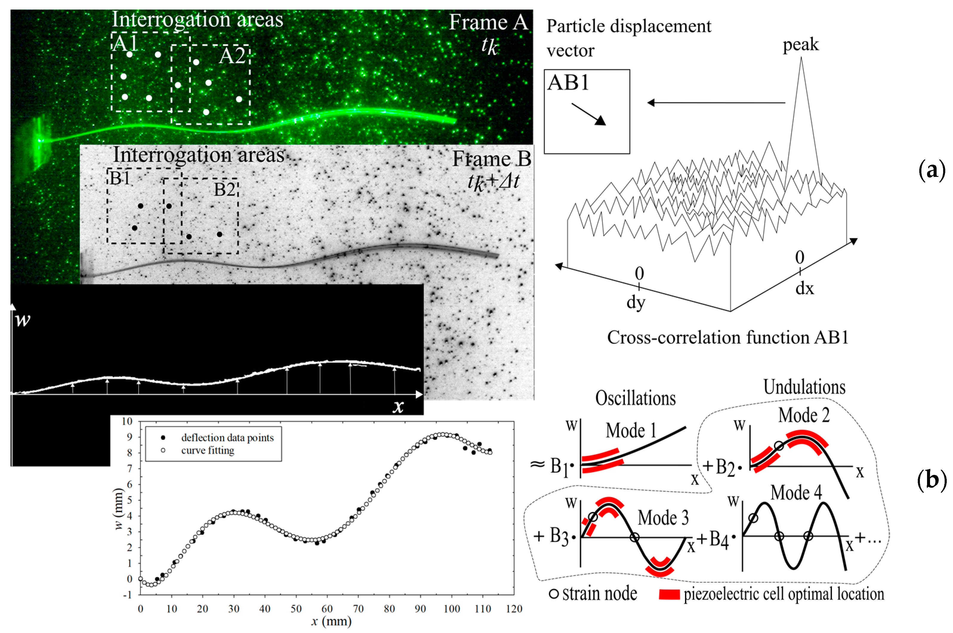
Energies 13 02645 g001
Figure 2. Experimental procedure: (a) particle image velocimetry principle; (b) shape capture, curve fitting and modal analysis.
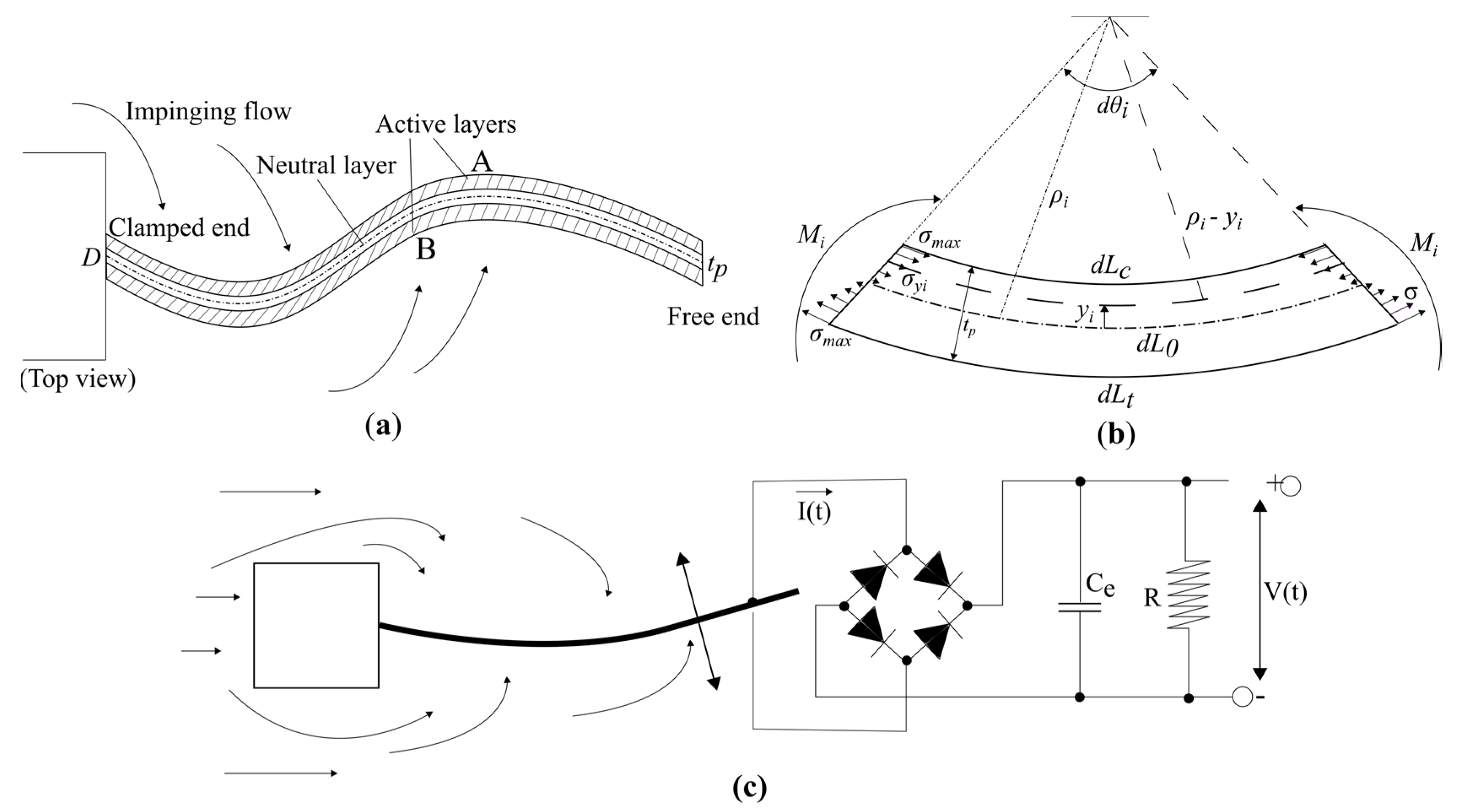
Energies 13 02645 g002
Figure 3. (a) Undulating plate in wake flow; (b) pure bending of the plate; (c) concept of the undulating piezoelectric energy harvester.
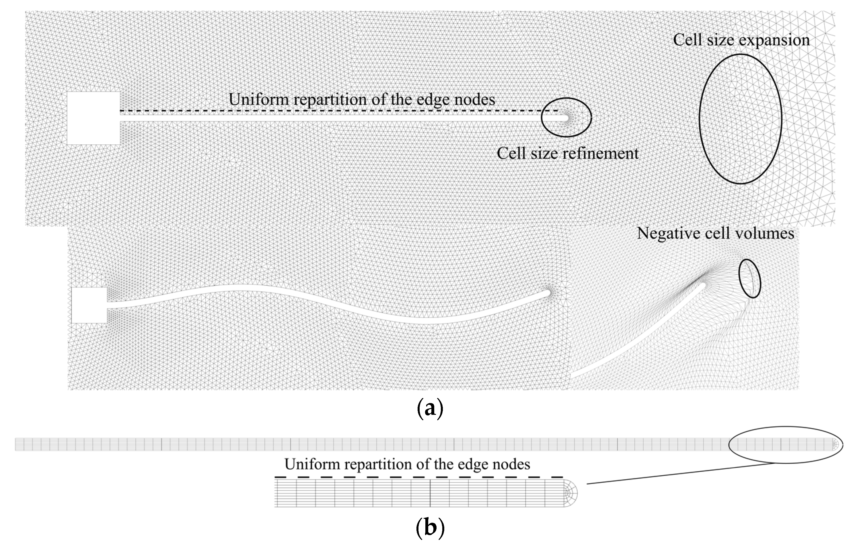
Energies 13 02645 g003
Figure 4. (a) Fluid mesh; (b) Solid mesh.
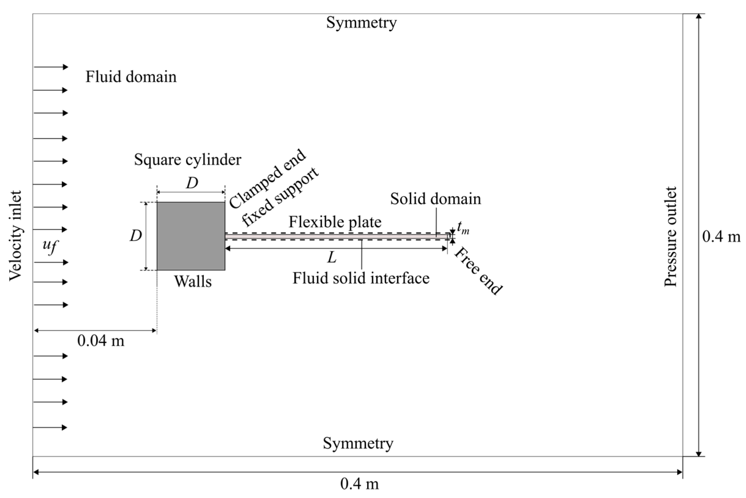
Energies 13 02645 g004
Figure 5. Boundary conditions for the fluid and solid domain.
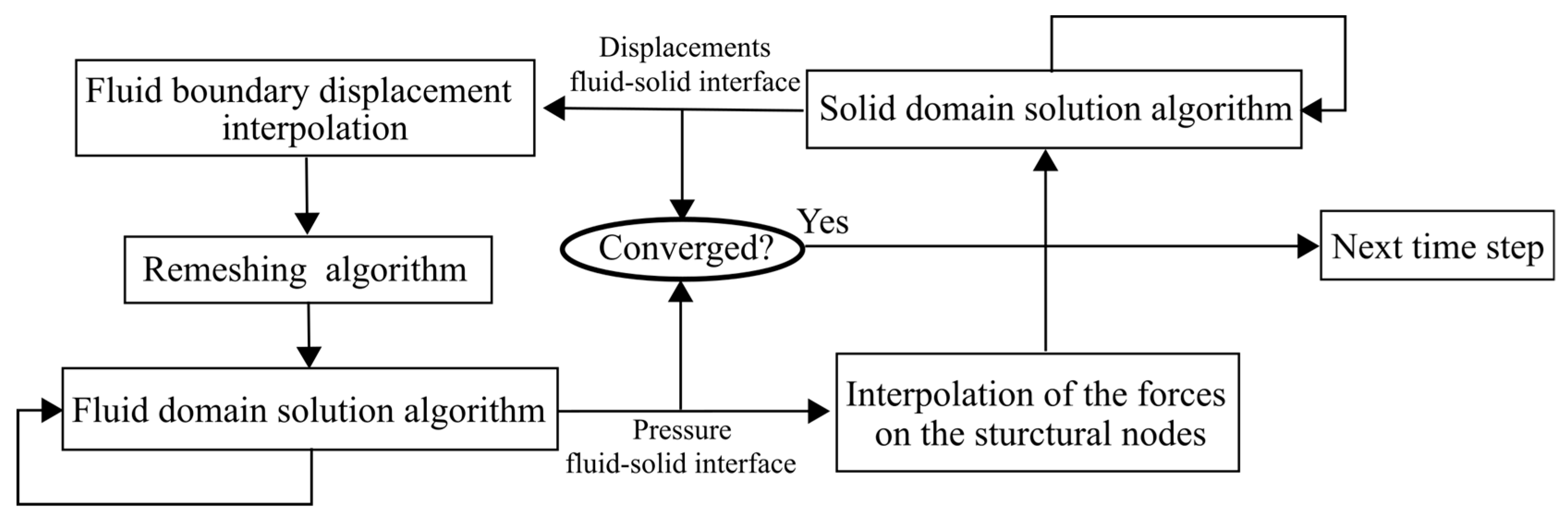
Energies 13 02645 g005
Figure 6. Fluid–structure interaction model stagger loop solution procedure.
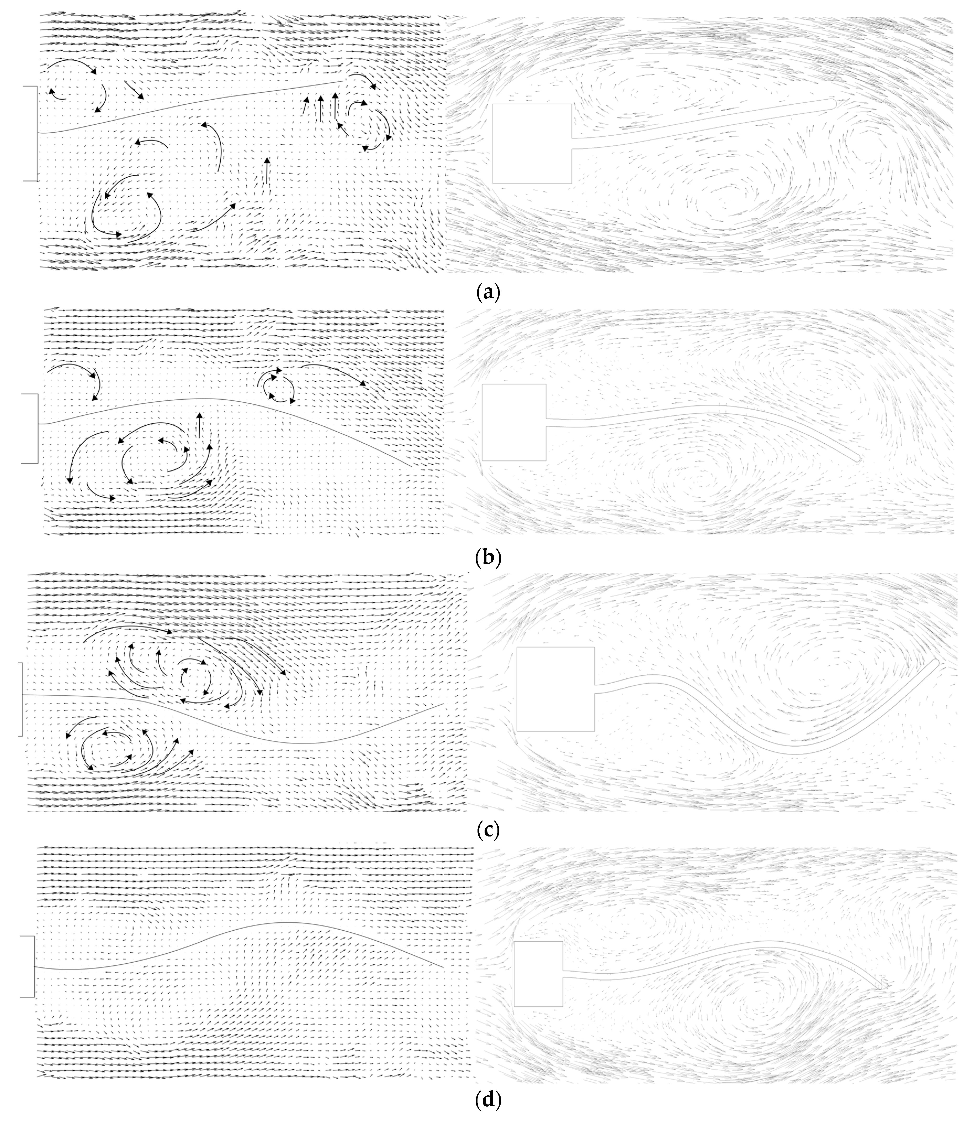
Energies 13 02645 g006
Figure 7. Comparison between the velocity vectors given by PIV and simulations for characteristic shapes, tp = 100 µm, W = 10 mm (a) L = 50 mm at RE = 12,295, (b,c) L = 75 mm at RE = 14,279, (d) L = 100 mm at RE = 14,279.
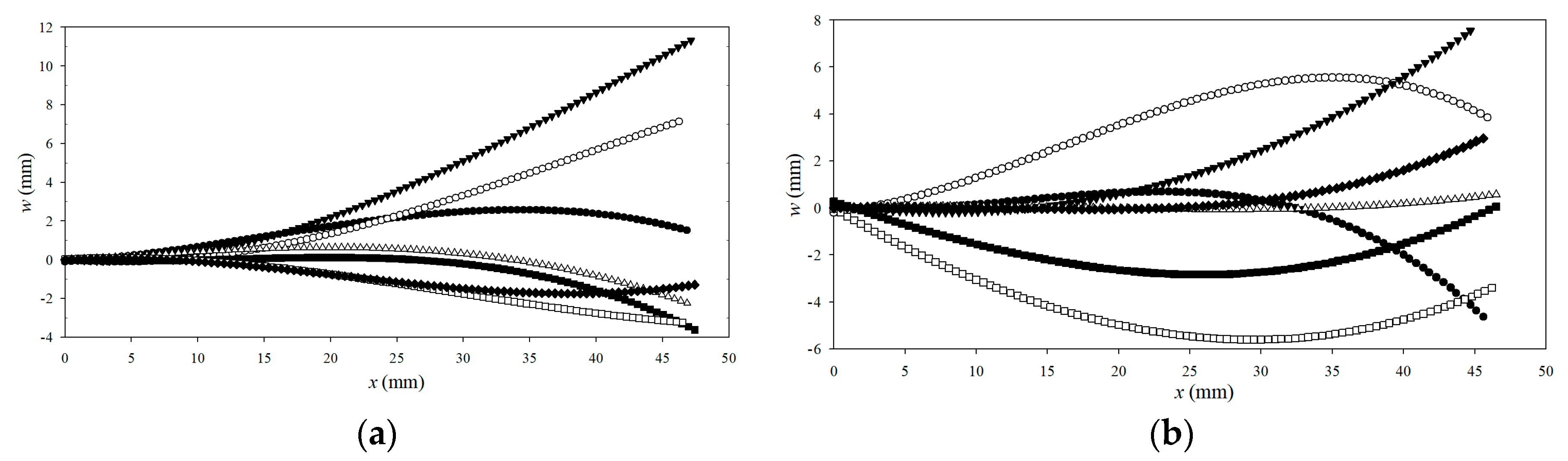
Energies 13 02645 g007
Figure 8. Water tunnel data characteristic deflected shapes tp = 80 µm, W = 5 mm, L = 50 mm (a) RE = 8025; (b) RE = 13,245.
Energies 13 02645 g008
Figure 9. Characteristic deflected shapes tp = 100 µm, W = 10 mm, L = 75 mm RE = 14,279 (a) Water tunnel data; (b) FSI model results.
Energies 13 02645 g009
Figure 10. Characteristic deflected shapes tp = 100 µm, W = 10 mm, L = 100 mm RE = 14,279 (a) Water tunnel data; (b) FSI model results.
Energies 13 02645 g010
Figure 11. (a) Bending power evolution with the Reynolds number from water tunnel experiments, and FSI model results highlighted with the arrows; (b) high-strain-energy shape recorded at RE = 9202 L = 50 mm plate; (c) high-strain-energy shape recorded at RE = 9202 L = 125 mm plate.
Energies 13 02645 g011
Figure 12. Water tunnel data. (a) Vortex shedding frequency and flapping frequencies of the plates; (b) Square cylinder vortex shedding-frequency-to-flapping-frequency ratio.
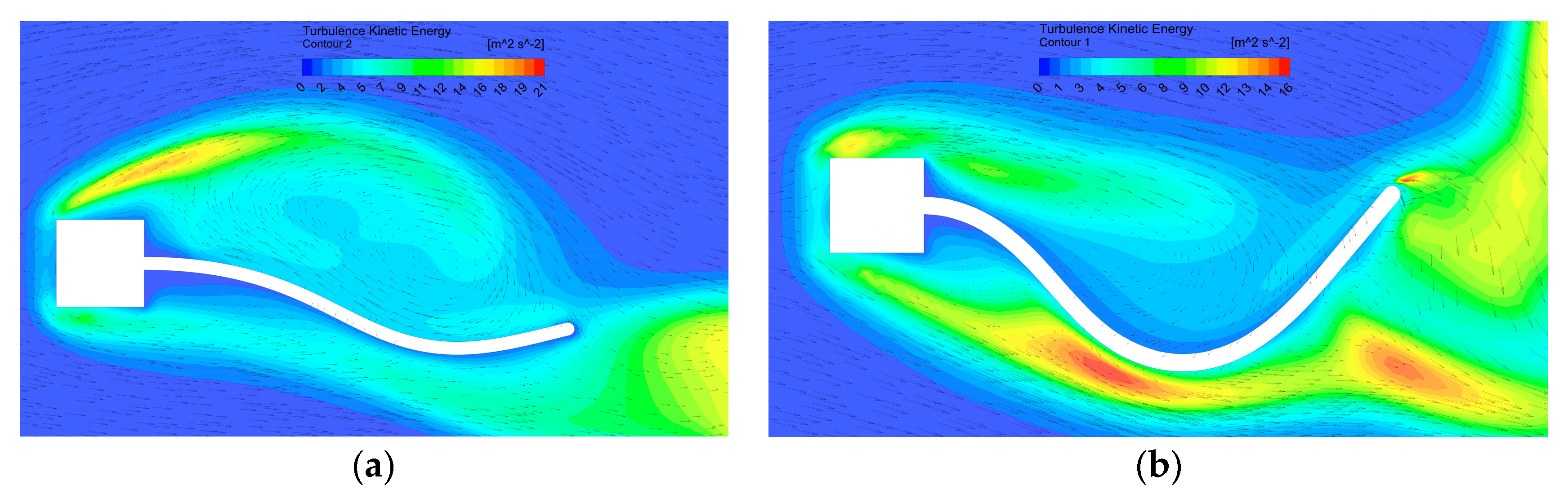
Energies 13 02645 g012
Figure 13. Turbulent kinetic energy contours (m2/s2) and velocity vectors for higher strain energy shapes at uf = 14.3 m/s.: (a) D = 10 mm, RE = 9648; (b) D = 8 mm, RE = 7718.
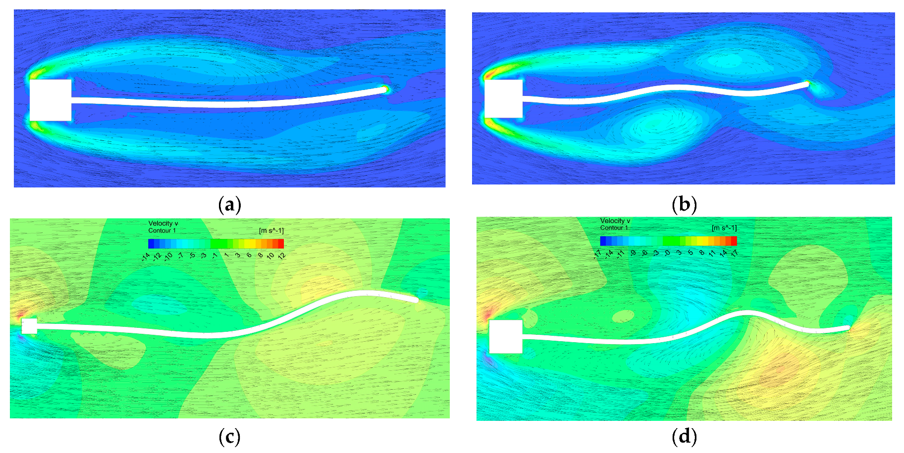
Energies 13 02645 g013
Figure 14. Velocity vectors and vorticity contours for high-strain-energy shapes for the plate L = 75 mm, D = 10 mm, tp = 100 µm, at (a) RE = 6218; (b) RE = 12162; transversal velocity v magnitude contours (m/s) and velocity vectors for high-strain-energy shapes, plate L = 100 mm, tp = 100 µm, at (c) uf = 20 m/s, RE = 5405, D = 4 mm; (d) uf = 20 m/s, RE = 16,216, D = 12 mm.
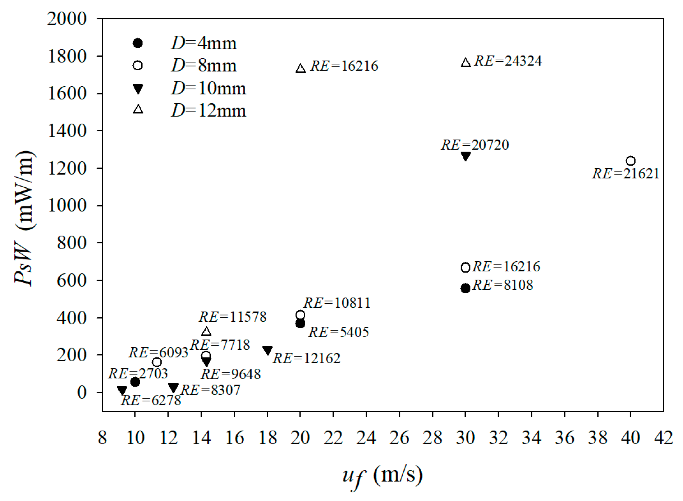
Energies 13 02645 g014
Figure 15. L = 100 mm, tp = 100 µm, Power per width evolution with the incoming fluid velocity and square cylinder diameter D.
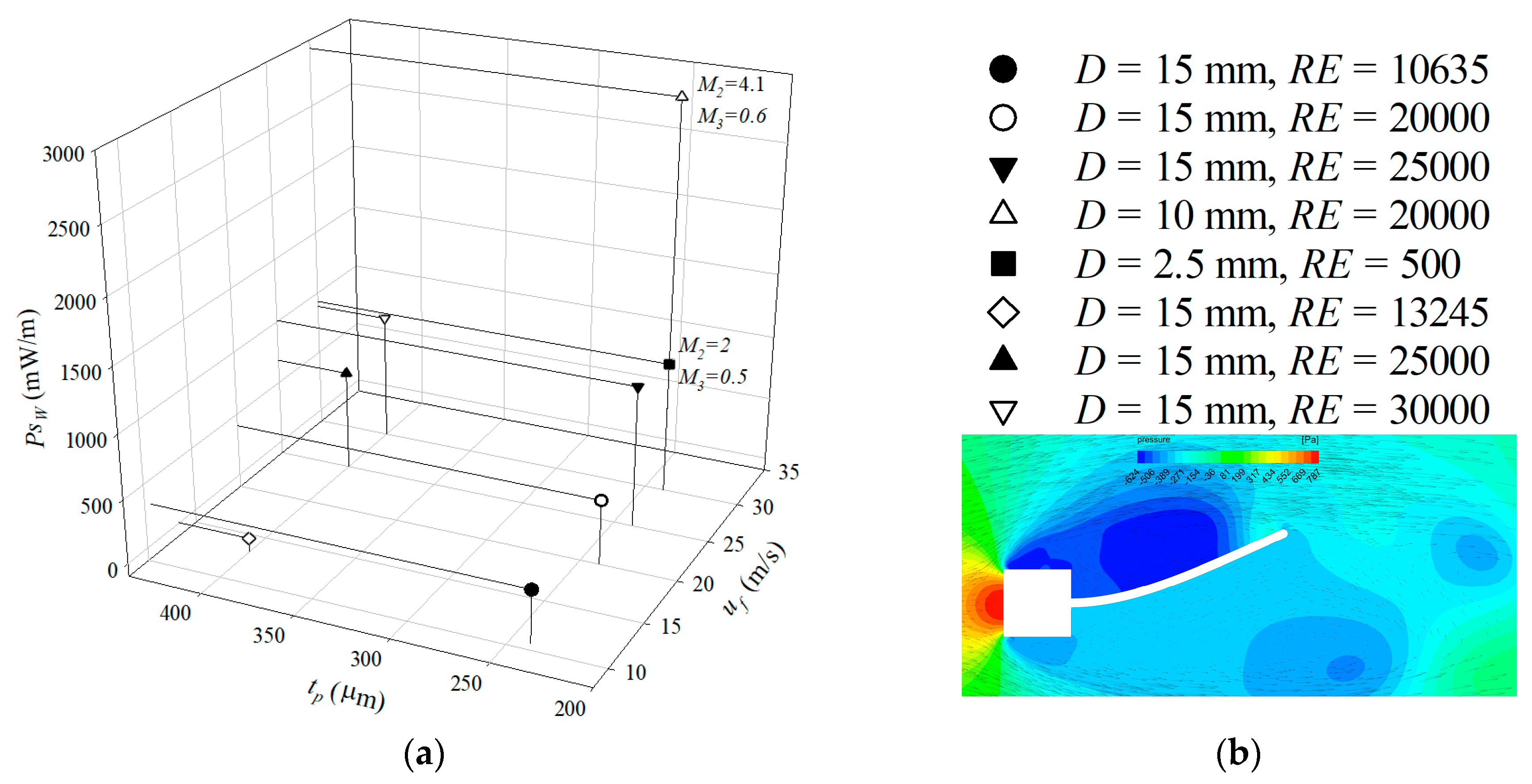
Energies 13 02645 g015
Figure 16. (a) Bending power PsW evolution with thickness and incoming velocity for L = 50 mm; (b) Mode 1 shape dominant bending pattern for the L = 50 mm, D = 15 mm, uf = 30 m/s, tp = 400 µm, highest strain energy shape, pressure contours and velocity vectors.
Energies 13 02645 g016
Figure 17. L = 50 mm, D = 10 mm, uf = 30 m/s, RE = 20,000, tp = 240 µm plate: (a) Characteristic deflected shapes; (b) stress distribution on the outer fiber for the deflected shapes.
Energies 13 02645 g017
Figure 18. Bending power PsW evolution with thickness and incoming velocity for L = 100 mm.
Energies 13 02645 g018
Figure 19. L = 100 mm, D = 8 mm tp = 600 µm plate, uf = 40 m/s, RE = 21621: (a) characteristic shapes; (b) stress distribution on the outer fiber for the above shapes.
Energies 13 02645 g019
Figure 20. Vortex shedding for the L = 100 mm, tp = 600 µm plate at uf = 40 m/s, (ac), D = 8 mm (d), (e,f) D = 12 mm.
Energies 13 02645 g020
Table 1. Fluid properties at atmospheric pressure.
Fluid at 20 °C ν f   ( m 2 / s ) ρ f   ( kg m 3 )
Air 1.5 · 10 5 1.2
Water 10 6 998
Table 2. Plate properties for the water tunnel experiments.
E   ( Gpa ) ρ p   ( kg m 3 ) t p   ( μ m ) W   ( mm )
21794805
2170110010
2147512010
Table 3. Properties of piezoelectric PVDF.
d 31   ( p C / N ) ε p σ   ( F m ) ε 0   ( F m )
23.9 [29] 13 ε 0 8.85 · 10 12
Table 4. Averaged modal contributions ratio to mode 1 contribution, L = 100 mm.
REM1M2M3M4
11,27210.460.570.20
12,29510.770.490.27
Table 5. Averaged modal contributions ratio to mode 1 contribution, L = 125 mm.
REM1M2M3M4
11,27210.420.260.16
12,29510.510.230.25
Table 6. Modal frequencies of the plates.
L mm f n 1   ( Hz ) f n 2   ( Hz ) f n 3   ( Hz )
50744123
753.11955
1001.81131
1251.1720
Table 7. Simulations results for the plate L = 50 mm, tp = 100 µm.
D (mm) u f   ( m / s ) RE P s W   ( mW / m )
89.2497416
814.37718114
109.2621865
1011.37616200
1012.38307235
1014.39648394
Table 8. Simulations results for the plate L = 75 mm, tp = 100 µm.
D (mm) u f   ( m / s ) RE P s W   ( mW / m )
109.2621855
1011.3761697
1012.38307205
101812,162434
Table 9. Estimated piezoelectric power output for the plates L = 50 mm, L = 100 mm.
L (mm) R l   ( M ) P l 1   ( mW / m ) P l 2   ( mW / m ) P l 3   ( mW / m )
501013598-
505020740-
5010014021-
10010132105526
10050184132658
10010013279500
Table 10. Conversion efficiencies.
L mm η f a i r   % η f w a t e r   % η m   % η g   air   % η g   water   %
500.361.580.030.12
1000.642.540.030.1

