A Methodology for Dependability Evaluation of Smart Grids

Abstract

Smart grids are a new trend in electric power distribution, which has been guiding the digitization of electric ecosystems. These smart networks are continually being introduced in order to improve the dependability (reliability, availability) and efficiency of power grid systems. However, smart grids are often complex, composed of heterogeneous components (intelligent automation systems, Information and Communication Technologies (ICT) control systems, power systems, smart metering systems, and others). Additionally, they are organized under a hierarchical topology infrastructure demanded by priority-based services, resulting in a costly modeling and evaluation of their dependability requirements. This work explores smart grid modeling as a graph in order to propose a methodology for dependability evaluation. The methodology is based on Fault Tree formalism, where the top event is generated automatically and encompasses the hierarchical infrastructure, redundant features, load priorities, and failure and repair distribution rates of all components of a smart grid. The methodology is suitable to be applied in early design stages, making possible to evaluate instantaneous and average measurements of reliability and availability, as well as to identify eventual critical regions and components of smart grid. The study of a specific use-case of low-voltage distribution network is used for validation purposes.

1. Introduction

Nowadays, power grid infrastructures are not designed to support the upcoming transition towards decentralized and distributed energy system. Traditional grids are essentially radial and designed for centralized power generation [1,2]. In the last decades, these electric networks became widely interconnected with large-scale generating stations built to provide massive amounts of energy. However, this model proved to be unreliable and inadequate [3,4], having operated the same way for decades with characteristics that contributed to the frequent occurrence of blackouts in the last 40 years [5].

Despite the introduction of Information and Communication Technologies (ICT) in the power generation industry, this innovation is concentrated in central nodes and partially incorporated to remote substations, whereas remote terminals are almost entirely archaic [6]. Additionally, factors such as population growth, climate change, equipment failures, restrictions in power generation capacity, demand for resilience and the reduction of fossil fuels are identified as reason for the creation of a new infrastructure for power distribution [7].

In this context, the concept of Smart Grid arises as an intelligent power grid. This infrastructure is an enhancement of existing power grids enabling benefits such as: efficient transmission of electricity, better restoration of services under power disturbances, integration of power generation systems and security issues [8,9]. The integration of renewable energy with the existing power grid is one of the most important benefits when considering the application of a smart grid. The current renewable energy generators work from small-scale residential applications to large-scale installations bringing several challenges for the whole electrical power system. The effects of renewable energy introduction with its inherent variability induce vulnerabilities to the system, requiring sophisticated security mechanisms. Thus, in order to make all these aspects beneficial to customers, it is necessary to ensure that a distribution system is capable of satisfying distributed scenarios (a large number of geographically spread generators with intermittent and stochastic generation), while meeting high reliability, resilience, efficiency and sustainability requirements [10,11].

Therefore, due to the stringent fault tolerance requirements imposed on power grids, quantitative evaluations are recommendable to be carried out even in the initial steps of power grid project. An early assessment of potential problems in a power grid, considering their probabilities, makes them easier to prevent and ensures continuity of power supply. The dependability analysis of smart grid infrastructure represents a valid approach to face this. Dependability can be understood as the ability of a system to avoid failure in the most critical services by combining and integrating attributes such as reliability, availability, maintainability, integrity and security properties [12]. Dependability analysis evaluates the ability of a target system to avoid service failures that can cause large losses, much higher than acceptable. Analyzing dependability of a system aims to determine its potential weaknesses and to improve its correct operation [13]. Currently, dependability analysis has been applied to many critical systems, such as national defense, aircraft, communications networks and many others [14,15,16].

Historically, dependability evaluation solutions in a smart grid context have been implemented focusing on Monte Carlo simulation [17,18]. Using this technique, there are contributions focused on distributed generation [19,20] and some simple models are proposed to energy storage [21]. On the other hand, alternative solutions based on probabilistic techniques emerged as a counterpoint to the Monte Carlo approach, aiming to reduce computational costs when compared to that simulation [22]. Considering smart grid scenarios, new analytic solutions for dependability evaluation should be developed emphasizing their feasibility for systematization, since smart grid analysis are in general difficult to execute due to the complexity of the grid infrastructure.

This work proposes, therefore, a methodology for dependability analysis of smart grids considering that components of distribution grid (transformer, distributed generators, feeders, ICT devices) are meant to fail and must be preventively repaired or replaced. The smart grid is represented as a graph where the hierarchical infrastructure is naturally modeled from an adjacency matrix. Regarding the analytic technique adopted in the methodology, Fault Tree (FT) formalism was chosen because of its flexibility and good suitability to modeling complex systems. The FT evaluation will be performed by sharpe, a tool widely used in literature [23], and a software that provides a graphical interface and a textual procedure (programming language) to describe and evaluate modeling paradigms as FTs. A case study encompassing a model adaptation of an European low voltage distribution network is then used to validate the proposed methodology [24].

The main contribution of this work is a flexible methodology that can be entirely automatized to evaluate smart grids dependability. The proposed methodology can handle any infrastructure topology (islanded and grid-connected operation), different fault conditions and load prioritization, besides being able to support distributed generation and energy storage. The strategy adopted in the proposed methodology can deal with any component (power grid and ICT components) by modeling it as generic vertex of a graph. Furthermore, the proposed methodology supports any quantitative analysis admitted in the fault tree formalism and any evaluation metric available in sharpe tool.

The remainder of this paper is organized as follows: Section 2 presents a recent literature review regarding the subject; Section 3 provides a brief description of dependability and state of the art. The methodology is presented in Section 4, while results are discussed in Section 5. Finally, Section 6 concludes the paper and presents directions for future studies.

2. Related Works

Interesting works related to assessment of dependability in smart grids have been developed in recent years and they are mainly focused on security [25,26,27] and network integrity [28,29,30,31]. Since smart grids have the ability to establish bidirectional digital communication, and for that use information technologies, they are susceptible to cyber attacks. Because of this, many studies review cybersecurity issues, focusing on preventing attacks and network breaches that may be favored to potential vulnerabilities of control and communication systems [32,33,34]. However, few studies on assessing the dependability of smart grids considering their physical infrastructure and different supplies of power generation can be found in the literature. In [18], the authors developed a simulation model able to perform such assessment, nevertheless, conditions and evaluation scenarios are explored in a restrictive approach, not supporting common mode failures or network fault conditions. Furthermore, the authors used the fault tree formalism to evaluate dependability and proposed an interesting strategy to construct a simpler fault tree for a smart grid, but they did not present an automated way to accomplish it.

There are studies also performing reliability evaluations on modern distribution systems using renewable generation or hybrid energy storage [17,19,20,21]. These studies applied the Monte Carlo simulation method to compute quantitatively the system reliability indices including the influence of islanded operation mode. However, the Monte Carlo approach is a more time-consuming method, being difficult to scale the analysis to bigger scenarios. The same problem can be also found in [18] as discussed before.

An approach concerning the best strategy to face failure scenarios in transmission lines of a smart grid was conducted in [35]. The authors used a generic model based on Markov chains to evaluate cascade failures. When considering failures in transmission lines, this work provides an important contribution. However, the technique created by the authors is restricted to reliability and resilience analysis and there is no modeling for other metrics such as availability or importance measures.

Another strategy for examining the dependability of a smart grid is to model the grid as a graph. Vertices of the graph would act as physical infrastructure components of the smart grid while the edges would be the transmission lines. Dependability analysis in a graph has been addressed by transforming a graph into a fault tree [14]. Moreover, that strategy considers the use of a generic fault condition based on the two-terminal problem whereas smart grids context turned the analysis into a modified k-terminal problem. This problem is defined considering a grid with N devices and a set of K devices ($K\subset N$ and $\left|K\right|<\left|N\right|$), where K is a combination of a centralized device and K − 1 field devices. Setting a centralized device $s\in K$, k-terminal problem is expressed as a probability of existing at least one way in s for each field device K included. two-terminals problem is the case where K = 2. Thus, a smart grid has multiple generating sources (k) and one or more loads (centralizers in the case of the problem graph). This way it has been labeled as a new assessment class, the modified k-terminal problem.

From the above discussion, it becomes clear that the works already developed in the literature have provided only a partial solution to the problem, since they are not focused on the physical infrastructure of the smart grid. In addition, these works are very restrictive regarding the definition of fault conditions, evaluation metrics, loads priorities and topologies. Revisiting all these aspects, this work proposes a methodology to analyse dependability of smart grids that can be entirely automatized and is based on a validated approach in literature [14] limited only to industrial wireless sensor network context. To refine this methodology [14], it was necessary to incorporate the specific nature of smart grids by addressing the modified k-terminal problem (many sources and many loads), dealing with load prioritization and being concerned about resilient topologies. Section 4 will explore this methodology in more detail. Additionally, to highlight the contributions of this work,

Table 1. Summary of literature reviews closely related with the proposed methodology.

Reference	Findings	Limitations	Comparing with Proposed Methodology
[14]	A methodology to analyze dependability of wireless sensor networks using a fault tree-based formalism and graph modeling.	The fault condition is based on two-terminal problem, because of its application scenario. Smart grids are modeled by K-terminal problem.	It maps the K-terminal problem to the fault tree formalism applied to smart grids scenario.
[17,19,20,21]	Perform reliability evaluations on modern distribution systems including islanded operation analysis	Use a Monte Carlo simulation method that is more time-consuming	Use analytical techniques and can be entirely automatized
[18]	A simulation model to assess dependability of smart grids physical infrastructure.	No support to common mode failures or network fault conditions. An automatized way to generate the top event was not presented.	It handles network fault conditions and can be entirely automatized to generate the fault tree top event for a smart grid.
[35]	A Markovian model that calculates reliability of smart grids.	It does not handle availability or component importance analysis	Any evaluation metric supported by the fault tree formalism can be calculated, including availability and importance measures.

compares the mentioned studies of literature review with the proposed methodology.

3. Dependability and Fault Tree Analysis

In this section, we provide a brief introduction to dependability and fault tree analysis concepts. As was mentioned, these definitions are closely related to the proposed methodology.

3.1. Dependability

Dependability is a widely discussed concept in literature [12,36,37] with several definitions. The original proposition [36] defines dependability as the capacity to deliver service that can justifiably be reliable. According to [37], the term is used to describe that a system can be reliable under certain operating conditions for a specific period of time. In this paper, the assumed definition of dependability is given by the system’s capacity of avoiding failures in critical services [12]. This interpretation can be applied to smart grids context, where failures in critical services can cause power supply outage and result in severe consequences.

According to [12], the dependability concept comprises the following combined attributes:

• Availability: ability to provide correct service when required. In other words, it is the probability of a system being operational when required.
• Reliability: continuity of correct service, which may be read as the probability of a defect does not occur in a given period of time.
• Safety: absence of catastrophic consequences to users and environment.
• Integrity: absence of improper system alterations or without authorization.
• Maintainability: ability to undergo modifications and repairs.

These attributes must be quantified, making it possible to assess how reliable is a particular system. The importance of each of them is subjective and depends on the context of the evaluated application [38].

3.2. Fundamental Measures

System dependability can be essentially described by two fundamental measures: reliability and availability [39]. These attributes are well described in the following subsections.

3.2.1. Reliability

The reliability $R\left(t\right)$ of a system is the probability of a failure not occurring in the interval [0,t) [39]. Suppose without losing generality that a system has two states [12], as shown in Figure 1. The transition from operating state to faulty state is triggered by the failure rate function $\lambda \left(t\right)$.

Now, consider T as the time to failure of a system component. If T is a random variable defined by a Cumulative Distribution Function (CDF) $F\left(t\right)$, it follows that reliability is given by:

$$R\left(t\right)=P(T>t)=1-F\left(t\right)$$

(1)

It can be proved that $R\left(t\right)$ and $\lambda \left(t\right)$, which describes the instantaneous failure rate of a system component, are associated as given by the Equation (2) [40]:

$$R\left(t\right)=exp\left(-{\int }_0^t\lambda \left(u\right)du\right)$$

(2)

Another metric related to $R\left(t\right)$ is the Mean Time To Failure (MTTF). This measure is defined as the expected time $E\left(t\right)$ elapsed until the occurrence of the (first) system failure [39]. Formally, MTTF is given by [40]:

$$MTTF=E\left(t\right)={\int }_0^{\infty }tf\left(t\right)dt$$

(3)

3.2.2. Availability

The availability $A\left(t\right)$ of a system is defined as the probability of the system being operational at a instant t [39]. As well as the reliability, availability also can be described as a model having two states, as shown in Figure 2. However, after the occurrence of a system fault, this new model may be repaired (maintenance). The transition from a faulty state to an operating state is induced by the repair rate function $\mu \left(t\right)$.

Availability can be obtained in the same way as reliability, by replacing each event for the failure and repair rate functions ($\lambda \left(t\right)$ and $\mu \left(t\right)$, respectively). Supposing that $\lambda \left(t\right)$ and $\mu \left(t\right)$ have constant values, then it can be proved that $A\left(t\right)$ is expressed by [40]:

$$A\left(t\right)=\frac{\mu }{\mu +\lambda }+\frac{\lambda }{\mu +\lambda }{e}^{-(\lambda +\mu )t}$$

(4)

Assuming that n periods occurred (with working and failed states), the steady-state availability $A_{\infty }$ can be outlined by Equation (5) [40]. In this case, MTTF $=1/\lambda$ and MTTR (Mean Time to Repair) $=1/\mu$.

$$A_{\infty }=\frac{MTTF}{MTTF+MTTR}$$

(5)

3.3. Importance Measure

In dependability evaluations, importance analysis is usually adopted to determine the sensibility of a system measure on the variation of the component features [13]. Generally, some components are more important for the system reliability than others and importance analysis aims to classify and quantify how the reliability of a component influences the whole system reliability [40].

Still according to [40], the component importance measure can be applied since the design phase to the operational period of a system’s life cycle. During the system planning, the importance measures must help the designer to identify weak points (bottlenecks) and components that should be improved. During the operational phase, importance measures may be used to guide the inspection and the maintenance actions to the most important components.

Several importance metrics have been developed to measure the relative importance of a component, in comparison with others and with respect to the system [41]. This section focus on one of these importance metrics: the Birnbaum measure [42].

For better understanding, suppose a system with n independent components, wherein each component i has a reliability function $R_i\left(t\right)$. Birnbaum measure $I^B(i/t)$ describes the reliability importance of the ith component. This metric is defined as a partial derivative of the system reliability with respect to the component reliability i, as shown in Equation (6).

$$I^B(i/t)=\frac{\partial R\left(t\right)}{\partial R_i\left(t\right)};i=1,2,\dots ,n$$

(6)

If $I^B(i/t)$ is a high value, a small variation of component i reliability will result in a considerable deviation of system reliability. A component i is critical to the system if its fault implies a system fault. Thus, Birnbaum measure can also be interpreted as the probability of a component being critical to the system at time t [40]. Namely, Birnbaum importance evaluates the probability of a system being in a critical condition with respect to a certain event (component fault) [43].

3.4. Fault Tree Analysis

The fault tree model is a resource applied to dependability analysis. It is a tree structure model representing a sequence of components’ individual failures that can cause a system breakdown. The first step to implement a fault tree is to determine a unique and well defined undesirable event, which is the top event and also is the single FT output [44]. In other words, the top event represents a system failure.

In general, FTs are graphical models representing a combination of events that are responsible for causing a system failure. The model uses a tree structure consisting of events and logic gates. The events represent the normal conditions as well as system failures (components failures, environmental conditions, human errors, and many others) and implement the boolean logic, i.e., they occur or do not occur. On other hand, the cause-effect relationships between events are represented by logic gates. A gate input can be a single event or a combination of events originated from the output of another logic gate [44]. In addition, there are several types of gates available on the formalism, like and, or and k-out-of-n gates.

Regarding assessment issues, Fault Tree Analysis (FTA) is an effective technique to evaluate qualitatively and quantitatively systems’ reliability and availability [45]. To perform qualitative analysis, FTA depends on the system stage. The development stage aims to identify potential problems that can lead to failures. In commissioning stage, the FTA technique can be used to identify the failure causes. Conversely, during the quantitative analysis process, it is possible to measure the reliability and availability of a system under assessment.

The main advantages of FTA are the execution of an intuitive procedure to describe the events that lead to system faults, and the minimization of the state space explosion problem, very common when modeling large systems [44].

The evaluation of a fault tree is performed by calculating the top event (system failure condition) probability based on basic events probabilities. This calculation is conducted differently for each type of logic gate. Assuming n independent inputs/events, the occurrence of event i is described by its cumulative distribution function $F_i\left(t\right)$. The logic gates outputs are indicated in Figure 3. When an and gate is used, the failure condition is only enabled when all inputs/events occur. On the other hand, the output of an or gate is enabled when at least one of its inputs/events is active. Finally, if a k-out-of-n gate is used, the output is enabled if at least k inputs/events occurred.

The equations presented in Figure 3 refers to a fault tree without repeated events. When repeated events occur, the equations are invalidated, hence, a different technique such as Sum of Disjoint Products (SDP) can be applied [46].

The SDP method can be efficiently applied to fault trees with repeating events and it is easily automated. The basic idea is to find a boolean function $\varphi \left(x\right)$ describing the system fault condition (top event) and transform it to a different function whose individual terms are mutually exclusive. According to [47], this structural boolean function $\varphi \left(x\right)$ is given by:

$$\varphi \left(x\right)=\left\{\begin{array}{cc}\hfill 1& \mathrm{system} \mathrm{failed}\hfill \\ \hfill 0& \mathrm{system} \mathrm{is} \mathrm{working}\hfill \end{array}\right.$$

(7)

where x is defined as the state vector, $x=(x_1,x_2,\dots ,x_n)$. Each element $x_i$ is a boolean variable, that represents the component state i.

4. Methodology for Dependability Evaluation

The proposed methodology aims to evaluate the dependability of a smart grid based on a fault tree model. In other words, by applying this methodology it will be possible to calculate a particular load’s reliability and availability. Still at grid design stage, the methodology may be used as an information provider (it needs grid topology, devices priority, redundancy level, and others as data input) to create a more robust and reliable infrastructure. The same information can also be used during the operating stage and grid expansion phase.

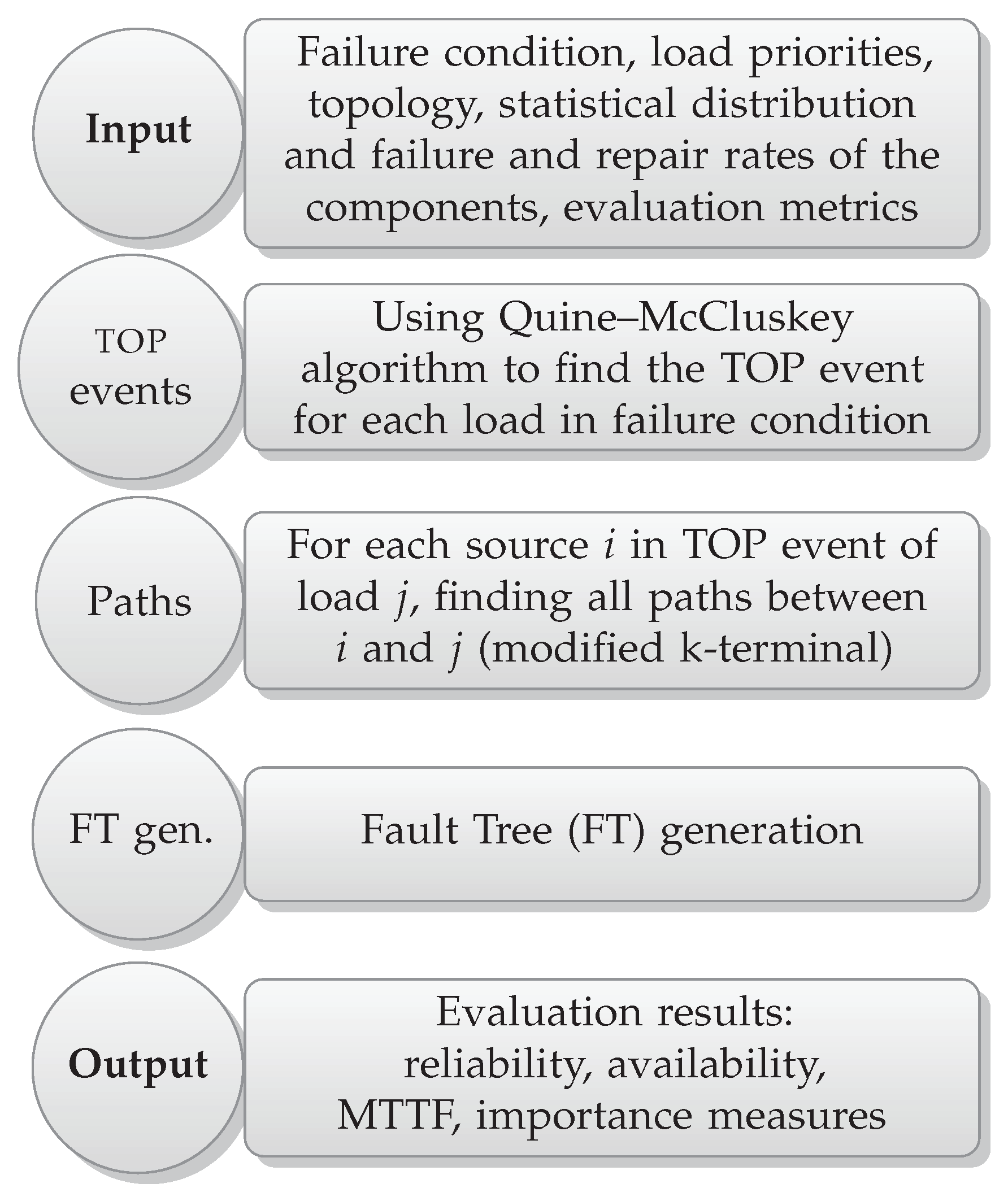
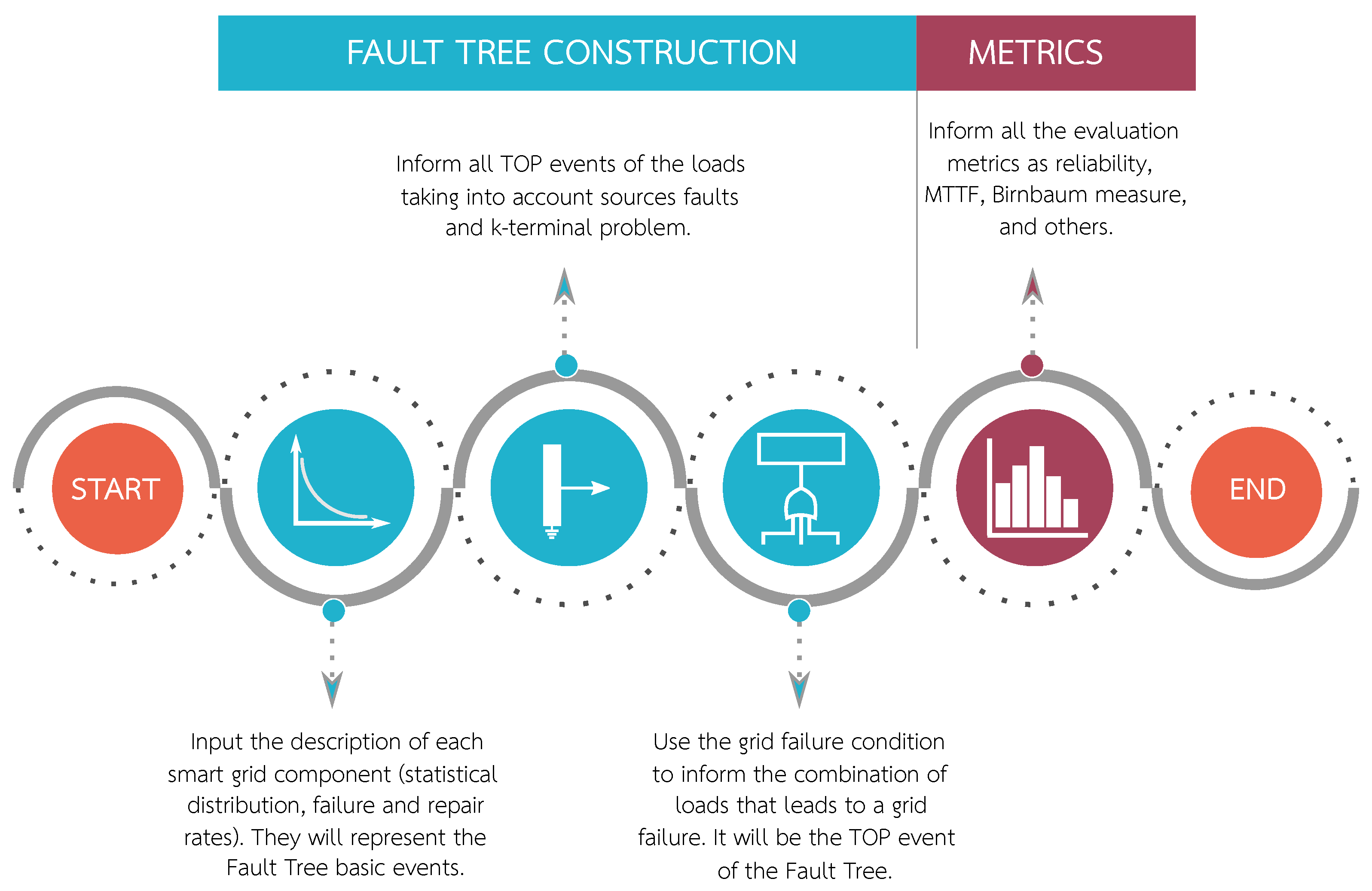
Figure 4 shows a methodology overview. The process begins by providing information about the grid topology, components failure and repair rates, evaluation metrics, loads prioritization and grid failure condition. It is worth mentioning that the grid failure condition is a logic expression that corresponds to the fault states of smart grid loads for a given scenario. Additionally, loads prioritization is a crucial information mainly in case of power supplies failure, when some loads may have higher priority than others. Turning back to the methodology’s big picture, the next step is to simplify the boolean expressions representing the different combinations of energy sources faults by applying the Quine–McCluskey classical algorithm [48]. The simplified expressions are the loads top events that comprise the energy sources situation. At this point, it is desirable that the methodology also handles more flexible failure conditions by incorporating the potential faults in the path between power supplies and loads. In this regard, an approach based on the modified k-terminal problem is performed to integrate the grid topology situation to the loads top events expressions. The resulting logical expressions are combined by the failure condition and transformed into a fault tree that can be processed by any FTA resolver (software). In this work, we adopted the sharpe tool as solver, because it is widely used in academia and provides analytic or symbolic approaches to compute the required metrics [23]. We also decide to use the sharpe’s textual procedure instead of the graphical mode because the first one is easier to automatize and as intuitive as the graphical interface. After considering that, the generated fault tree can be inputted into SHARPE using the textual syntax without having any adaptation in the FT logical expression.

4.1. Data Input

This section describes each methodology data input required for dependability evaluation.

4.1.1. Topology

The initial stage of the process consists in the definition of the optimal data structure which will model the smart grid topology. In this work, the grid is represented as a graph $G(V,E)$ with n vertices (V) and k edges (E). The vertices represent the physical components of the smart grid infrastructure while the edges represent communication links. The grid topology is stored in a adjacency matrix ($M_{n\times n}$) of the graph G. If a component $N_i$ has a neighbor $N_j$, then the $m_{ij}$ and $m_{ji}$ entries of M will be one, otherwise they will be substituted by zero. Within this approach, any smart grid topology can be represented as a graph (adjacency matrix).

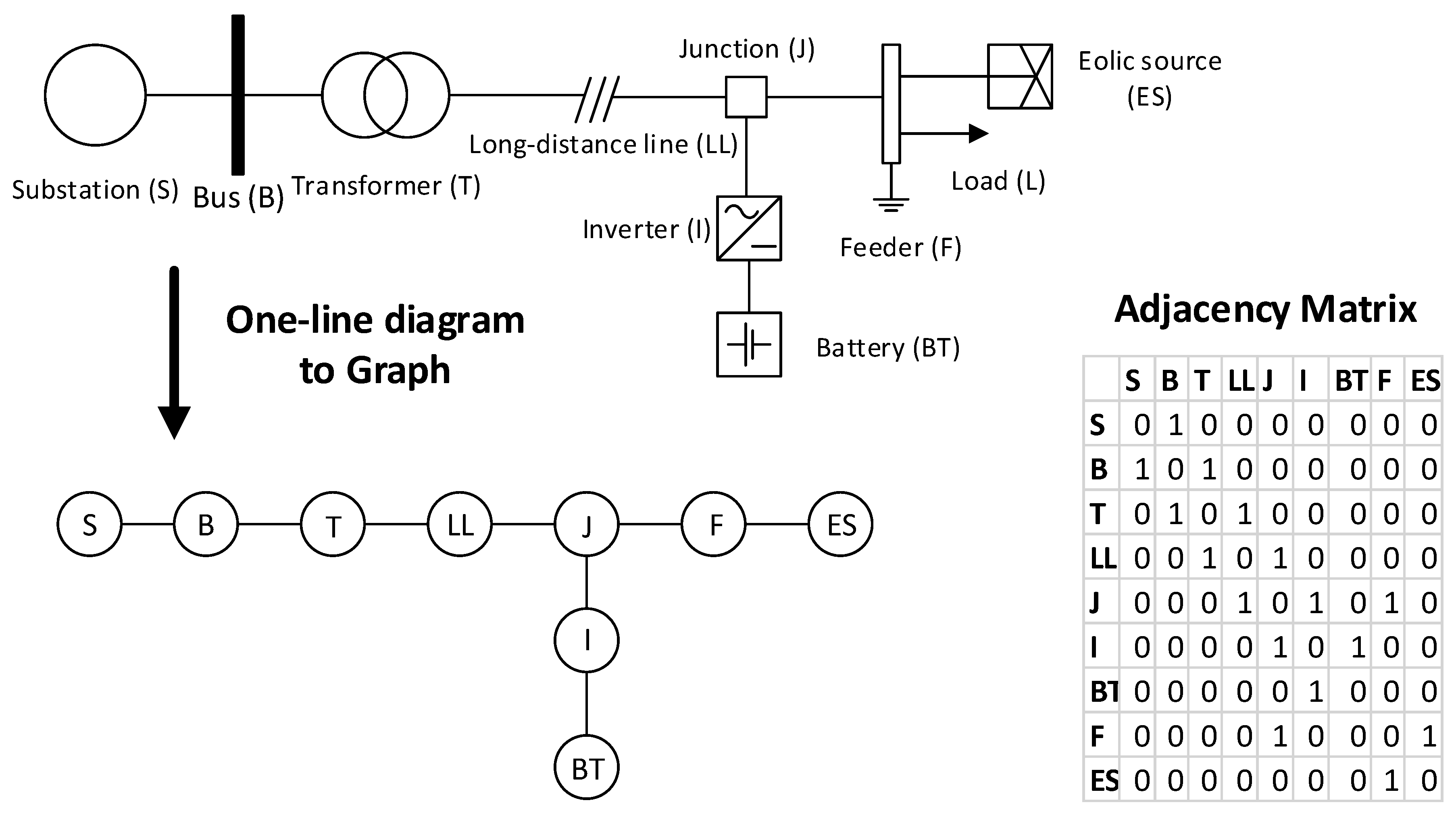
For the sake of understanding, the Figure 5 describes the procedure to transform an one-line smart grid diagram into a graph representation. Note that the on-line diagram’s components are typical of smart grid scenarios [49]. Although no ICT component is shown in Figure 5, we highlight that any type of component can be modeled since an element of the graph has a generic representation.

4.1.2. Fault Settings

The proposed methodology is able to handle the permanent fault of physical infrastructure components of a smart grid and of its transmission lines. After a permanent fault, a grid device is considered permanently inoperative. To be operational again, a repair process must be performed. This work assumes that repairs are independent and they are limitless. Also, a load is inoperative if for any reason its energy demands can not be met.

At first any probability distribution can be used for modeling fault and repair processes. However, sharpe tool was adopted to perform quantitative analysis and it requires that CDF of components should be expressed using exponential polynomials as described by Equation (8).

$$F\left(t\right)={\displaystyle \sum _{j=1}^n}{a}_j{t}^{k_j}{e}^{b_{j}t}$$

(8)

$a_j$, $k_j$ and $b_j$ terms are parameters of the exponential polynomial while e is the Euler number. $k_j$ is a non-negative integer and $a_j$ and $b_j$ are real or complex numbers. Many distributions can be expressed by Equation (8) (e.g., exponential, erlang, hypoexponential, hyper-exponential). Others non-exponential distributions (e.g., weibull, lognormal, deterministic) can be approximated using hybrid techniques involving a combination of moments and nonlinear least squares method [23].

4.1.3. Grid Failure Condition

Depending on the applications requirements, faults in specific devices can lead to failures in the entire grid. To perform more reliable analysis when applying the proposed methodology, it is fundamental to point out the loads combination which, in case of fault, leads to a grid failure.

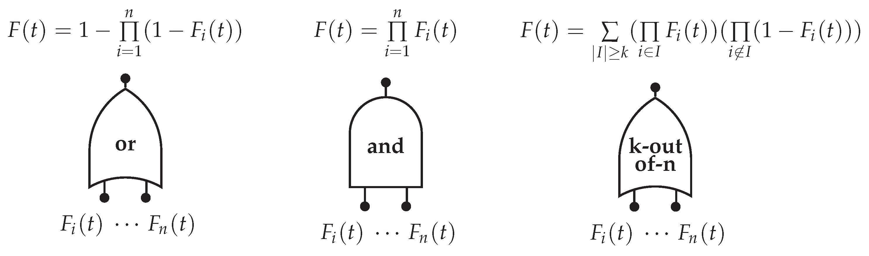
This methodology supports failure conditions whose combination of devices can be set using logic gates and, or or k-out-n. In practice, any configuration could be used.

4.1.4. Priorities

Load priorities are also represented in the methodology. Priorities are essential parameters because in case of a fault, loads with higher priority are met first. The prioritization should be determined to provide a systematic sequence of service that satisfies the system conditions. Electrical system loads can have different priorities depending on its importance in the system. Priorities determination is guided by the requirements that the grid designer and the system operator decide to adopt.

4.1.5. Evaluation Metrics

The evaluation metrics that can be calculated using the proposed methodology are: reliability, availability, MTTF, and component importance measures. Some of these metrics need supplementary information to be evaluated. For instance, to estimate reliability, MTTF, and components importance measures, it is necessary to inform the elements failure rates and their probabilistic distributions such as those mentioned before.

4.2. Top Event to the Loads

After defining the grid failure condition, it is necessary to find the top event for each load belonging to that condition. At this point, it is crucial that priority requirements are met. Thus, it is necessary to calculate all combinations of faults in the supplies that lead to a failure in a load.

Every load has a L demand while each supply has a S capacity. Without loss of generality, assuming two loads whose demands are $L_1$ and $L_2$ (the first load priority is higher than the second one), two supplies with $S_1$ and $S_2$ capacities, the following failure scenarios can be identified:

• Load 1

  -

  $L_1>\sum$ active sources

• Load 2

  -

  $L_2>(\sum$ active sources) − $L_1$

Based on this logic, a truth table can be created where input events are the supplies and output events are the loads. The classic Quine–McCluskey (Karnaugh mapping) algorithm can be used to simplify the boolean functions for each load [50]. This simplification is advised to make logical expressions simpler and consequently to reduce the evaluation time. As result, we find the top event for each load.

4.3. Modified k-Terminal Problem

The top event described in the previous section is a function of the smart grid supplies. However it is still necessary to consider the grid topology and therefore faults in connection elements and transmission lines. Assuming that the grid failure condition refers to k devices, then the dependability quantitative analysis falls into the classic k-terminal reliability problem.

The first step is to find all the paths between a energy source and a load i. This procedure can be performed using a Depth-First Search (DFS) to traverse the whole adjacency matrix representing the topology from a target load to a power supply, as described in Algorithm 1. Thus, all the paths between a given supply and a load must be found. If at least one path is operational, the supply is considered operational. A path fails if at least one of its elements fail.

Algorithm 1: Finding all paths between a load and a energy source.

4.4. Construction of Fault Tree and Evaluation

The final step of the proposed methodology is the construction of the fault tree and its respective evaluation.

The construction strategy of the fault tree basically includes three steps as shown in Figure 6. Firstly, each component of the smart grid must be defined in terms of its statistical distribution and its failure and repair rates. These components then represent basic events of the fault tree. After this, the next step is to list all the top events of the loads obtained previously. They are simplified expressions of the loads that comprise the energy sources and the topology situations. Finally, the top event of the fault tree will be the grid failure condition representing the combination of loads that leads to a grid failure.

Once the fault tree is constructed, we can provide the chosen metrics to perform the analysis. The metrics used in the evaluation are the reliability and the availability of the smart grid as well as the criticality for a particular grid component.

5. Results

To validate the proposed methodology, we will describe a case study involving a microgrid. A microgrid is a plug-and-play small-scale system operating under low or medium voltage, having distributed generation and loads. Microgrids allow smart grid concepts to be applied in the current power supply system and can operate concomitant with main grid (connected to the grid) or independently (isolated mode of operation). The operation in isolated mode is performed when the main grid is disturbed by main power supply faults. In this case, the microgrid can disconnect itself from the main grid and operates in isolated mode, continuing to supply the loads through distributed generators, regardless of problem occurred at the power distribution utility.

5.1. Assumptions

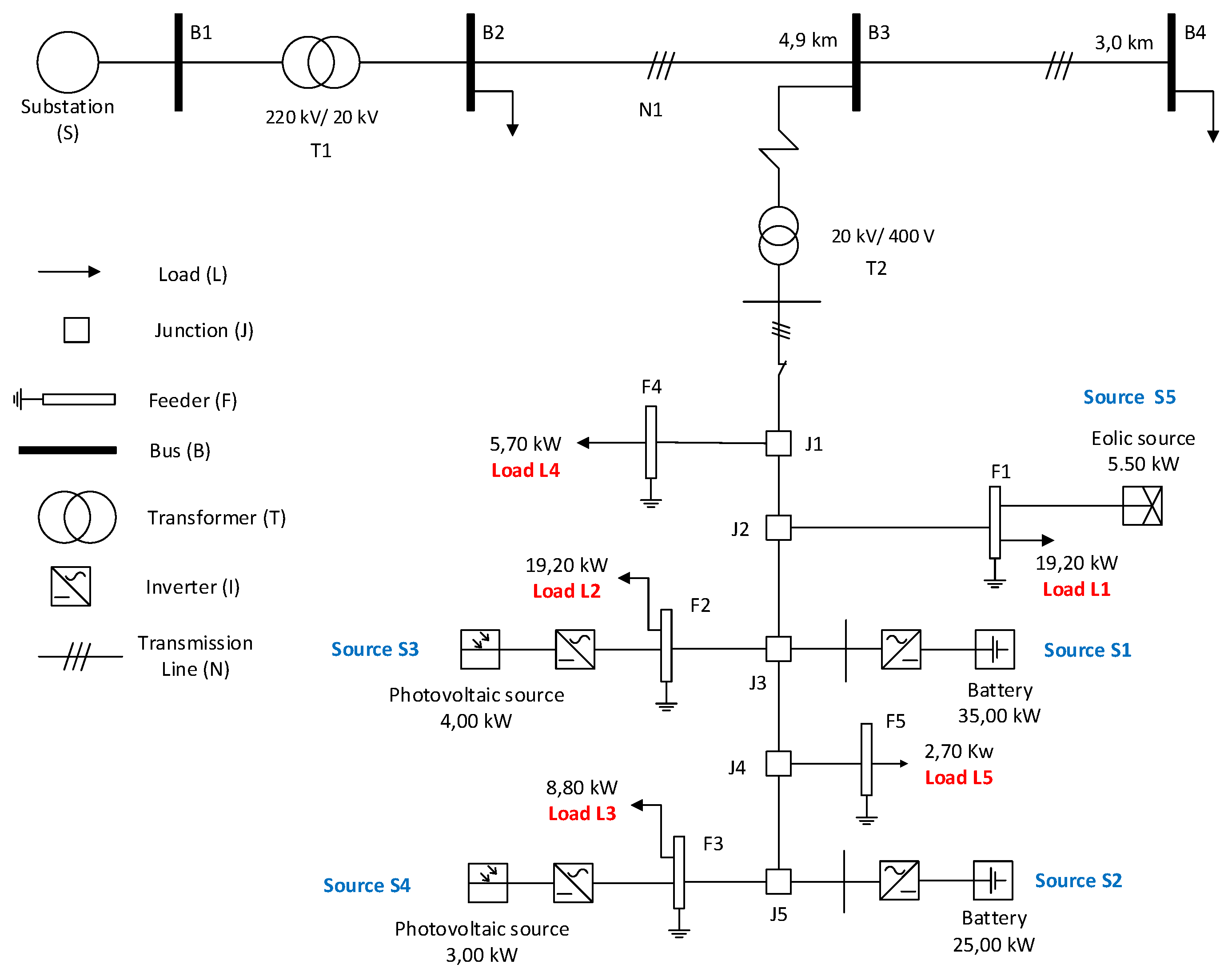
A single-line diagram describing the case study is presented in Figure 7. The system is composed by five loads ($L1,L2,L3,L4,L5$) with priority defined as $L1>L2>L3>L4>L5$. It also has five power supplies ($S1,S2,S3,S4,S5$). For the sake of simplicity, the inverter component was not considered in the evaluation.

The objective of the study is to analyze the microgrid dependability (probability of load loss and expected load cuts) for the third bus ($B3$) using the proposed methodology. This evaluation is performed considering that the microgrid connected to $B3$ disconnects from the medium voltage distribution grid when faults occur in the following components: 220 kV/20 kV transformer, medium voltage grid sections (4.9 km line), 20 kV/400 V transformer, distributed generation (solar, wind and batteries) and junctions $J1,J2,J3,J4,J5$. In the isolated mode of operation, a fault occurs in the microgrid when there is insufficient generating capacity to meet the original load demand.

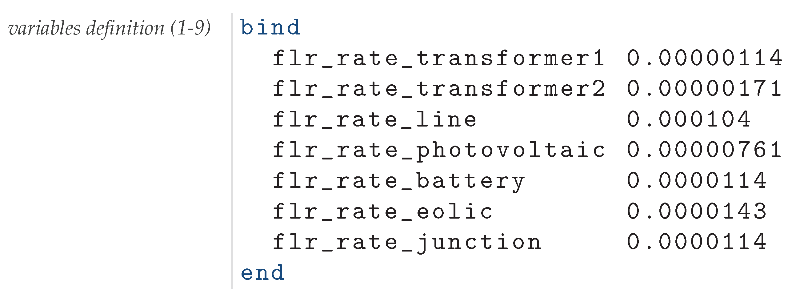
Regarding the study scenario, some issues concerning the faults and metrics rates also need to be considered: (1) the evaluation metrics to be considered were the reliability and MTTF of microgrid, and the components importance measure; (2) the fault rates of system components are distributed exponentially (other distributions can be used, as long as exponential polynomials are used to describe them, as required in sharpe tool) and the time unit is hours. Fault rates adopted in this study comply with typical values found in literature [44] and are described in

Table 2. Typical failure rates of smart grid components.

Component	Failure Rate	MTTF
4.9 km Line	1.04 × 10−4	1.09 years
220 kV Transformer	1.14 × 10−6	100 years
20 kV Transformer	1.71 × 10−6	67 years
Photovoltaic Source	7.61 × 10−6	15 years
Battery	1.14 × 10−5	10 years
Eolic Source	1.43 × 10−5	8 years
Junctions	1.14 × 10−5	10 years

.

These fault rates were informed to sharpe by using its intuitive textual procedure as shown in Figure 8. In this code, each component’s fault rate was associated to a variable. For instance, the flr_rate_transformer1 has the value 1.14e-6 and refers to the failure rate of the 220 kV transformer.

5.2. Top Event of Loads

A main step in the methodology is the top event building for the loads in the evaluated scenario. This step involves load prioritization and consequently total generation of distributed sources, which are designed to supply all demand. Total generation of distributed sources for the case study scenario is: ${\sum }_{i=1}^5{S}_i$ = 35.00 + 25.00 + 4.00 + 3.00 + 5.50 = 72.5 kW.

At this point, a truth table is created with the five supplies as inputs and the five loads as outputs. Therefore, each load will have one top event. Bear in mind that, in this work, the zero value represents that a element has not faults, i.e., it is operational, and the one value denotes the occurrence of a failure (a component is defective). Furthermore, it is well known that each row of the truth table has one possible combination of the input variables and the result of the evaluation for those values. Hence, with five sources, there is a total of $2^5$ configurations for the sources states, which may or may not lead to a load fault state. All of this configurations are needed to be considered in the top event building and they are described in

Table 3. Failure combinations.

Total (kW)	Sources (kW)					Loads (kW)
	S1	S2	S3	S4	S5	L1	L2	L3	L4	L5
	35	25	4.0	3.0	5.5	19.2	19.2	8.8	5.7	2.7
72.5	0	0	0	0	0	0	0	0	0	0
67.0	0	0	0	0	1	0	0	0	0	0
69.5	0	0	0	1	0	0	0	0	0	0
64.0	0	0	0	1	1	0	0	0	0	0
68.5	0	0	1	0	0	0	0	0	0	0
63.0	0	0	1	0	1	0	0	0	0	0
65.5	0	0	1	1	0	0	0	0	0	0
60.0	0	0	1	1	1	0	0	0	0	0
47.5	0	1	0	0	0	0	0	0	1	1
42.0	0	1	0	0	1	0	0	1	1	1
44.5	0	1	0	1	0	0	0	1	1	1
39.0	0	1	0	1	1	0	0	1	1	1
43.5	0	1	1	0	0	0	0	1	1	1
38.0	0	1	1	0	1	0	1	1	1	1
40.5	0	1	1	1	0	0	0	1	1	1
35.0	0	1	1	1	1	0	1	1	1	1
37.5	1	0	0	0	0	0	1	1	1	1
32.0	1	0	0	0	1	0	1	1	1	1
34.5	1	0	0	1	0	0	1	1	1	1
29.0	1	0	0	1	1	0	1	1	1	1
33.5	1	0	1	0	0	0	1	1	1	1
28.0	1	0	1	0	1	0	1	1	1	1
30.5	1	0	1	1	0	0	1	1	1	1
25.0	1	0	1	1	1	0	1	1	1	1
12.5	1	1	0	0	0	1	1	1	1	1
7.0	1	1	0	0	1	1	1	1	1	1
9.5	1	1	0	1	0	1	1	1	1	1
4.0	1	1	0	1	1	1	1	1	1	1
8.5	1	1	1	0	0	1	1	1	1	1
3.0	1	1	1	0	1	1	1	1	1	1
5.5	1	1	1	1	0	1	1	1	1	1
0.0	1	1	1	1	1	1	1	1	1	1

.

The first row of Table 3 refers to a combination in which there is no source faults (all columns have zero values). In this scenario it is possible to get the total generation capacity of the distributed sources (72.5 kW). On the other hand, the row with a total power of 47.5 kW presents a configuration where the source S2 has failed (the logical value for S2 column is 1). Therefore, total generation is now 72.5 kW − S2 (25.00 kW) = 47.5 kW. It is necessary to evaluate the load faults according to their priorities. Load L1 is supplied by 47.5 kW. Then, the remaining generation relative to other loads will be 28.3 kW (47.5 kW − L1, where L1 = 19.2 kW). The remaining generation is enough to supply L2 and L3, but not to supply L4 and L5. Note that L4 and L5 in Table 3 are marked with 1. Finally, configuration of row where total power is 37.5 kW allows just L1 load to be supplied.

Finally, it is necessary to apply the Quine–McCluskey algorithm to perform the boolean simplification and get the correspondent expression for each load according to the distributed sources. For all 32 combinations of Table 3, it is possible to get the following top events:

$$\begin{array}{cc}\hfill L1=& S1.S2\end{array}$$

(9)

$$\begin{array}{cc}\hfill L2=& S1+S2.S3.S5\end{array}$$

(10)

$$\begin{array}{cc}\hfill L3=& S1+S2.(S3+S4+S5)\end{array}$$

(11)

$$\begin{array}{cc}\hfill L4=L5=& S1+S2\end{array}$$

(12)

5.3. K-Terminal Problem

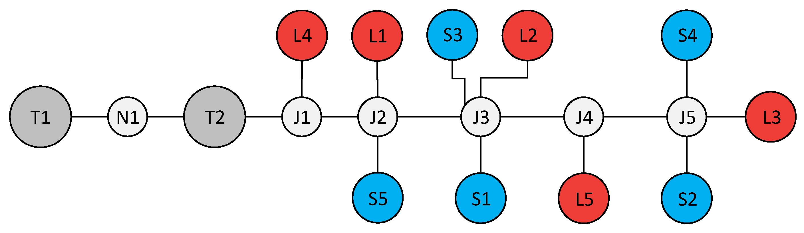
Equations (9)–(12) still do not represent the entire top event for the loads. They consider only faults in isolated mode of the microgrid. A downtime for a service occur if the main power supply and the isolated mode of a microgrid fail. Thus, it is necessary also to consider faults in transformers and junctions as well as topology aspects of a microgrid (k-terminal problem). The latter is only figured out from the graph model of the scenario under study (Figure 7) whose representation is described in Figure 9. Note that a path between a supply and a load fails if at least one element fails along the path.

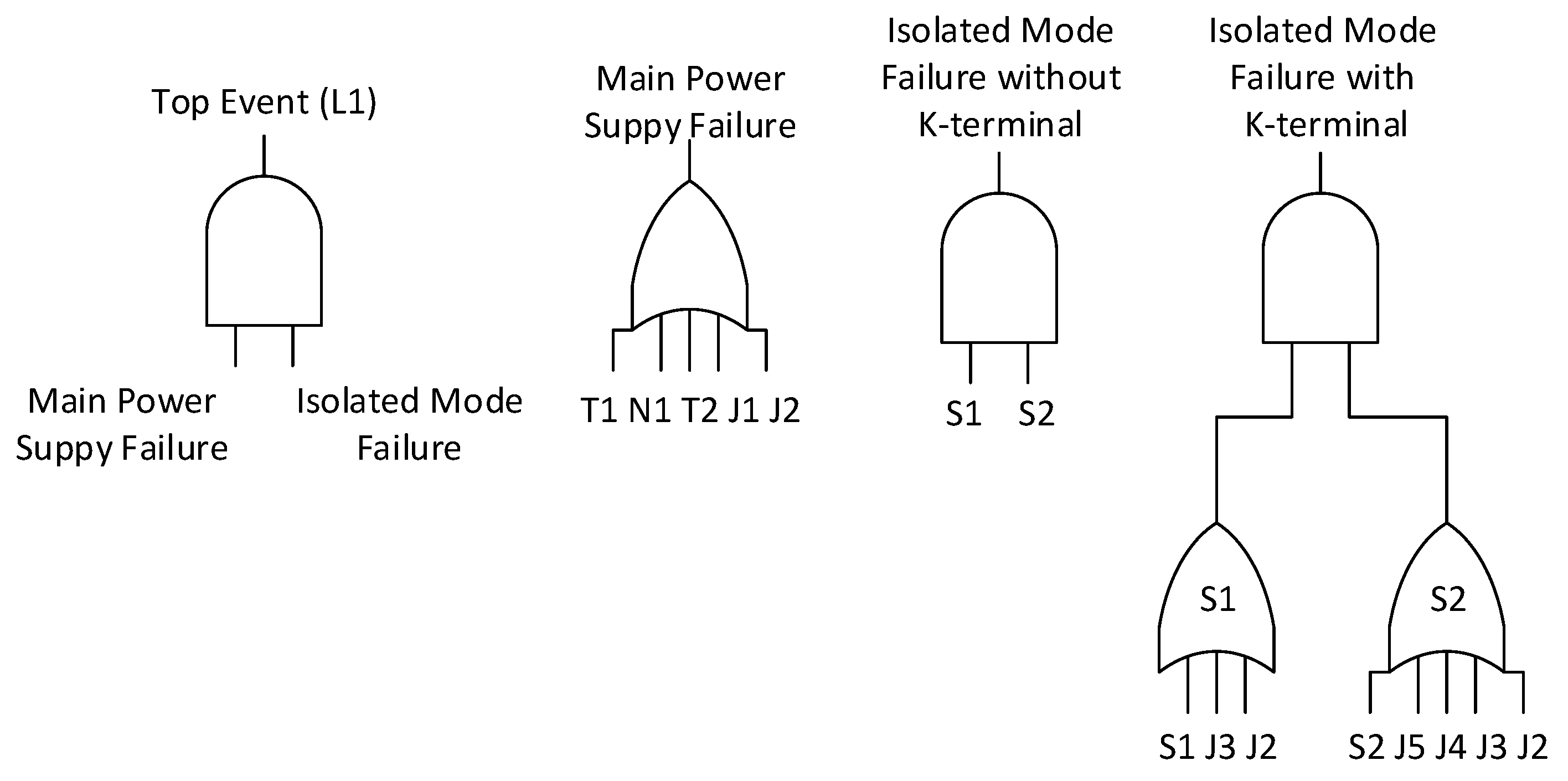
To simplify things, it is assumed that only junctions from $J1$ to $J5$ can fail. Additionally, assuming that faults in 220 kV/20 kV and 20 kV/400 V transformers are $T1$ and $T2$ respectively, and in the 4.9 km long transmission line is $N1$, the top event to load $L1$ can be found as described in Figure 10. Note that, as previously mentioned in Section 4.3, it was necessary to find all paths between the load L1 and the sources S1 and S2, which are contained in L1’s top event (isolated mode failure without k-terminal) showed in Equation (9).

It is also considered that due to the peculiarity of the system topology, only one path between a supply and a load exists. The top event for all loads can be deducted in following equations:

$$\begin{array}{cc}\hfill L1=& (T1+N1+T2+J1+J2)\\ \hfill & .(S1+J3+J2).(S2+J5+J4+J3+J2)\end{array}$$

(13)

$$\begin{array}{cc}\hfill L2=& (T1+N1+T2+J1+J2+J3)\\ \hfill & .\left(\right(S1+J3)+(S2+J3+J4+J5)\\ \hfill & .(S3+J3).(S5+J2+J3))\end{array}$$

(14)

$$\begin{array}{cc}\hfill L3=& (T1+N1+T2+J1+J2+J3+J4+J5)\\ \hfill & .\left(\right(S1+J3+J4+J5)+(S2+J5)\\ \hfill & .\left(\right(S3+J3+J4+J5)+(S4+J5)\\ \hfill & +(S5+J2+J3+J4+J5)\left)\right)\end{array}$$

(15)

$$\begin{array}{cc}\hfill L4=& T1+N1+T2+J1).((S1+J3+J2+J1)\\ \hfill & +(S2+J5+J4+J3+J2+J1))\end{array}$$

(16)

$$\begin{array}{cc}\hfill L5=& (T1+N1+T2+J1+J2+J3+J4)\\ \hfill & .\left(\right(S1+J3+J4)+(S2+J5+J4\left)\right)\end{array}$$

(17)

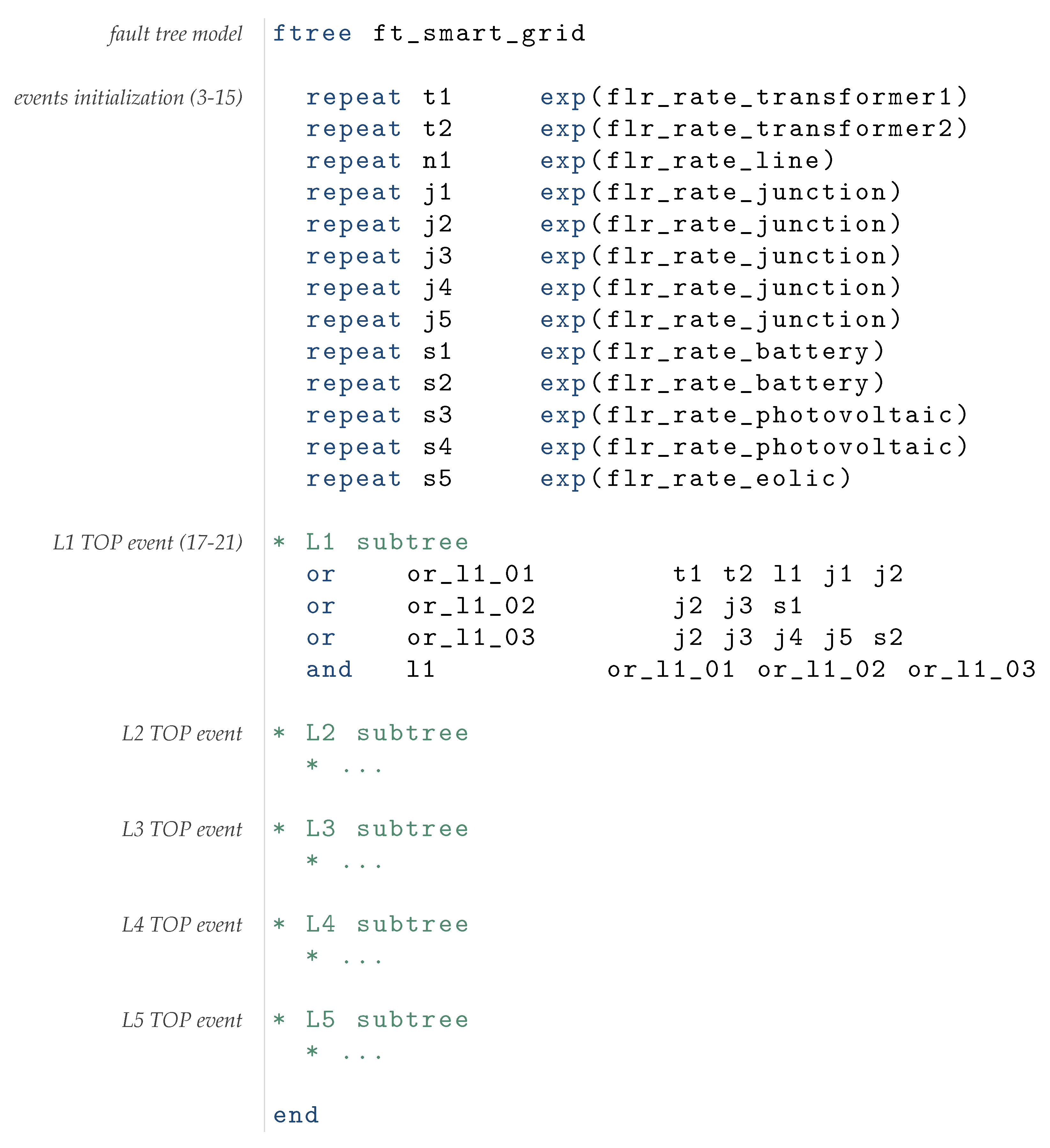
These top events of the loads were then input into sharpe tool as part of a fault tree. For the sake of better understanding, the code shown in Figure 11 implements the events representing components faults and the L1 top event. The first line initializes a fault tree structure. In sequence, the events are created with their types, names and fault rate distributions respectively. For instance, line 3 represents the T1 event mentioned before and describes it as a repeated event t1 (events are considered repeated when they occur more than once in a fault tree) exponentially distributed (exp function) with flr_rate_transformer1 as fault rate. Similarly, lines 4 to 15 correspond to the other events. Lines 17 to 21 presents the L1 top event indicated by Equation (13). In each line the gate type, name and inputs are informed respectively until composing the final top event expression. TOP events from other loads will be analogously implemented in the following lines before the end command.

5.4. Evaluation Metrics

This section describes two evaluation scenarios for the microgrid under study, in which concepts presented in this work are applied to. The objective is to evaluate different scenarios where all the features supported in the methodology can be validated, proving its wide application flexibility. As previously mentioned, the quantitative evaluation of fault tree generated by the methodology is solved by the sharpe tool. Scripts used in the experiments are available online for reproducibility purposes (https://github.com/gisliany/lii-system-ft).

5.4.1. Scenario I

In this first scenario, two fault conditions in the microgrid are confronted. Reliability and MTTF of the smart grid are calculated based on expressions describing top events for loads L1 and L2. The following fault conditions were considered:

• L1 + L2: the grid fail when at least one load is not fed;
• L1 $·$ L2: the grid failure occurs only when those two loads are not fed simultaneously.

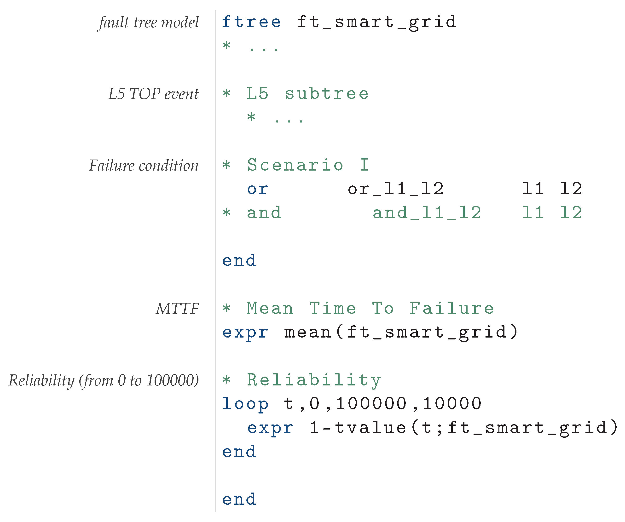
At this point, the fault conditions and the requested metrics (reliability and MTTF) are provided to sharpe. The script that specifies all these parameters is shown in Figure 12. Only one fault condition is evaluated at a time and it must be still specified inside the fault tree structure. In Figure 12, the fault condition L1 + L2 is enabled and the condition L1.L2 is commented in a line below to be computed in the next execution. The evaluation metrics are described right after the fault tree. The mean built-in function estimates the MTTF and the 1-tvalue function is repeated inside a loop from 0 to 100,000 (hours) to evaluate the reliability in this period of time.

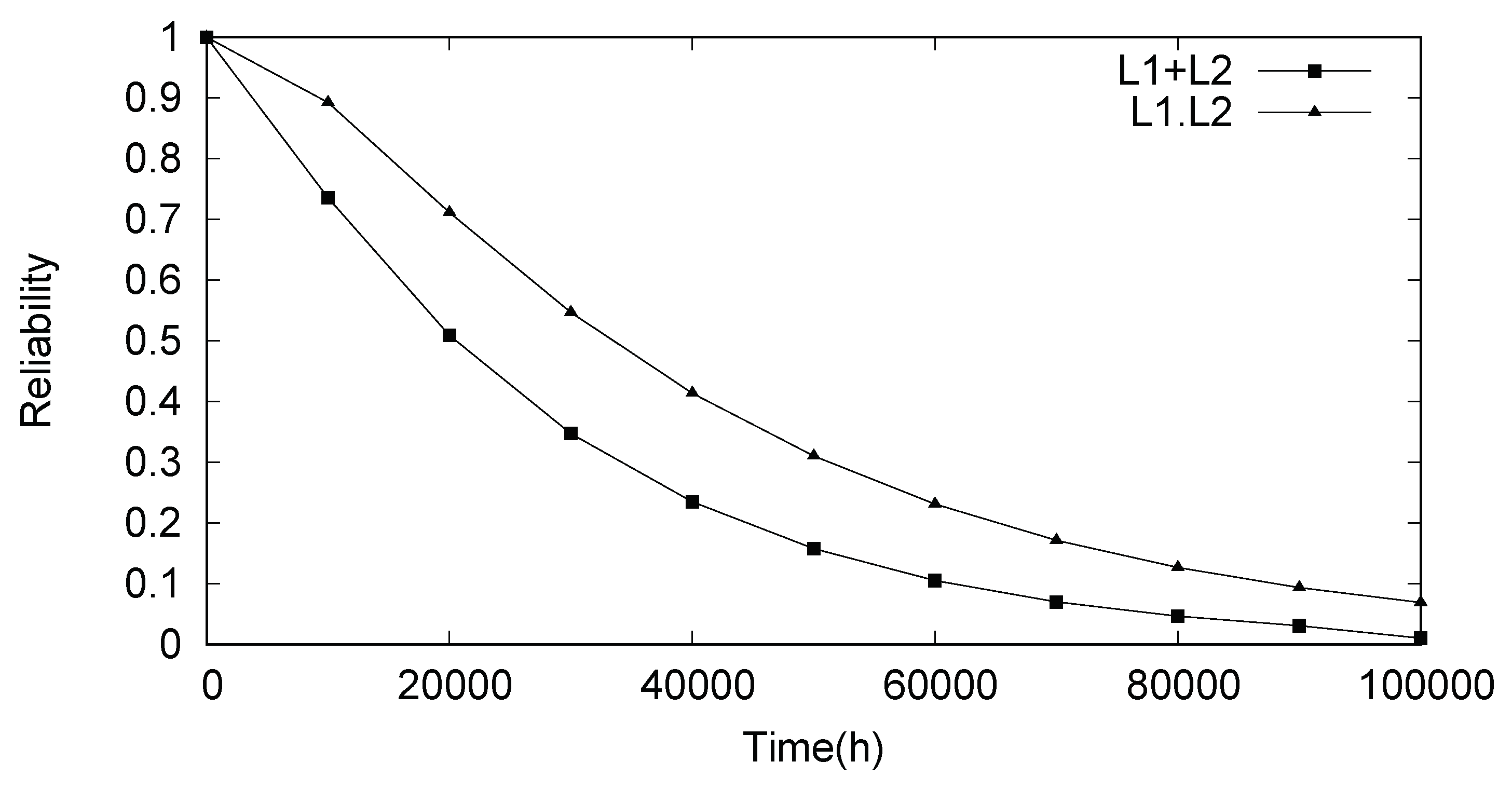
Reliability results for the two situations can be seen in Figure 13. Through the analysis of the generated curves, notice that $L1+L2$ condition is more pessimistic than the $L1·L2$ condition, since the first mentioned condition is more likely to occur. For instance, when t = 20,000 h, reliability for $L1+L2$ is $0.509$, whereas for $L1·L2$ condition, reliability reachs a higher value (0.711). The same happens to the MTTF. The former has a 3.16 years MTTF, while the latter provides a 4.85 years MTTF (a relative difference of 35%). This kind of evaluation can be useful to determine if a given failure condition reaches a specific dependability requirement in a microgrid project.

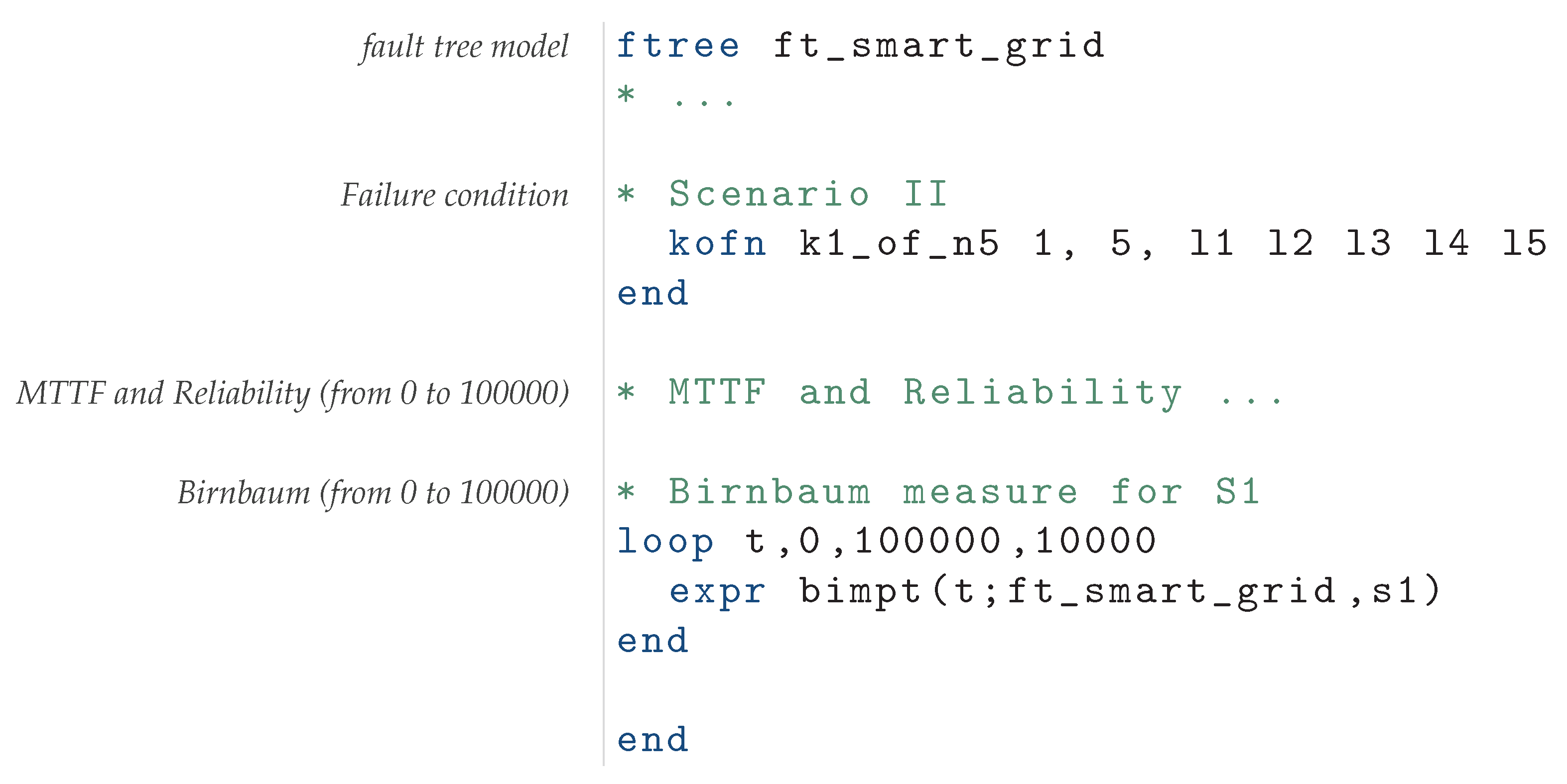
5.4.2. Scenario II

The second evaluation scenario leads with five different situations of fault condition considering all loads of the microgrid. For this evaluation, the logic gate k-out-of-n is used to represent the possible states for grid faults where k is the amount of loads that are not electrically powered by sources, or in other words, in fault conditions.

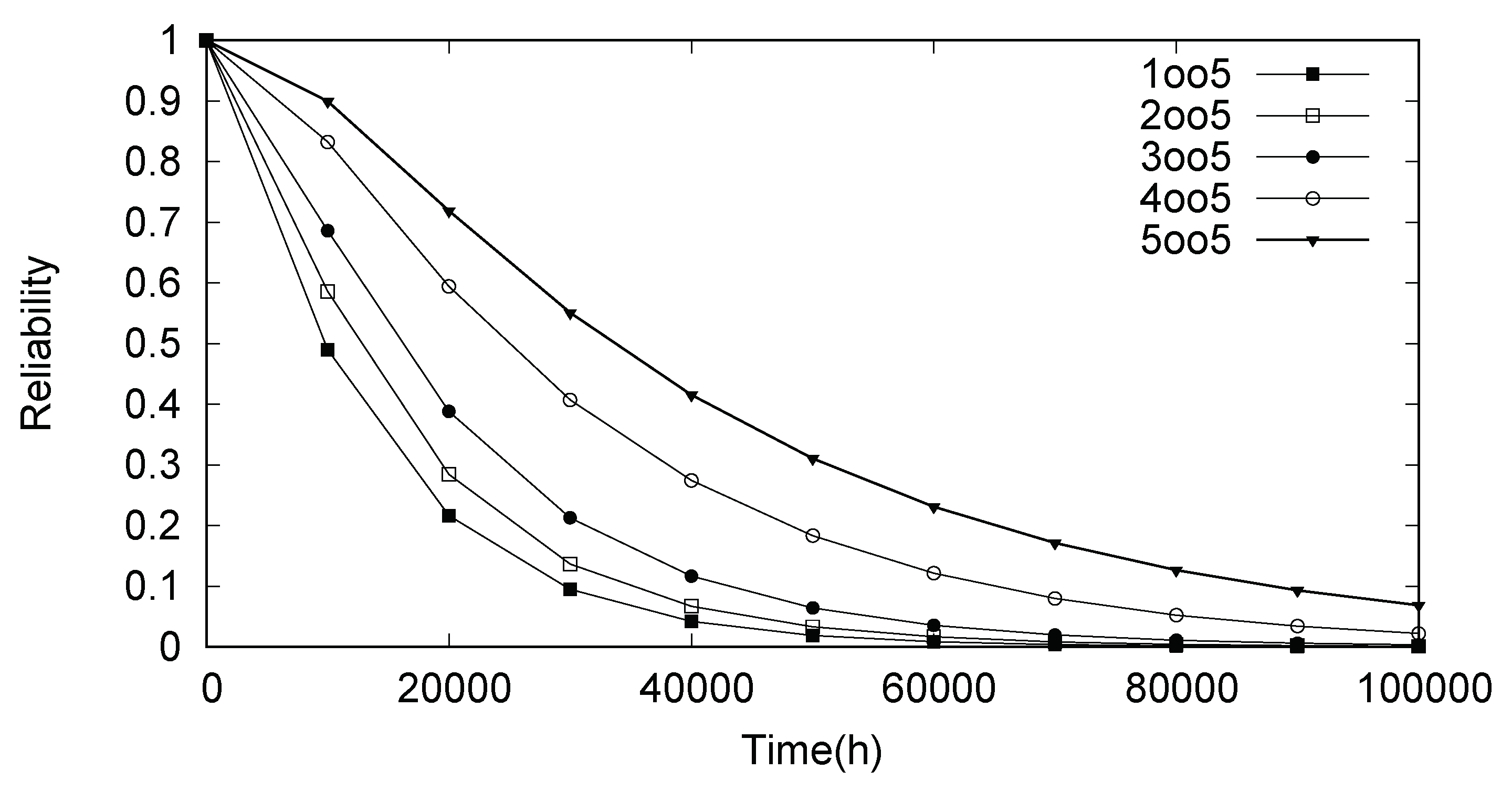
The use of the logic gate k-out-of-n allows to test a wider range of fault settings. In the case, as there are five loads, the use of this gate makes five defects conditions possible:

• Case I (1oo5), at least one load is not fed;
• Case II (2oo5), at least two loads are not fed;
• Case III (3oo5), at least three loads are not fed;
• Case IV (4oo5), at least four loads are not fed;
• Case V (5oo5), all loads are not fed.

For the sake of understanding, the sharpe code for the Case I is illustrated in Figure 14. This code is similar to that of Figure 12 and the only difference is the fault condition and appending the Birnbaum measure for S1 source as an example. In the case, the failure condition is specified by the gate type (kofn), name, k value, n value, and inputs.

Reliability results for each case is shown in Figure 15. As expected, analyzing the generated curves it is possible to conclude that the case wherein all devices failed (working as logic and gate) has a greater reliability since it is less likely to occur. It is clear that cases I and V are extreme, however, other cases can be used to delineate dependability limits for a specific microgrid project.

Similar to that observed in evaluation of scenario I, MTTF values for each case can be extracted. This analysis is described in

Table 4. MTTF evaluation for k-out-of-n fault condition.

Case	MTTF (h)	Increase over 1oo5
1oo5	1.327 × 104	-
2oo5	1.617 × 104	21.79%
3oo5	2.036 × 104	53.37%
4oo5	3.141 × 104	136.62%
5oo5	4.277 × 104	222.17%

. The relationship between the MTTF and the number of devices in fault condition (k value in k-out-of-n gate) is directly proportional. The greater the number of devices failing at the same time, the greater is the time to fail. Table 4 also presents a comparison of each case with the highest probability of occurrence (case I). In the most optimistic scenario (case V), the increase rate means that the time to failure more than doubles as compared to the most pessimistic scenario (case I). This result confirms the previous reliability evaluation described in Figure 15.

Another evaluation metric is the Birnbaum measure. This metric describes the importance of a component for the microgrid reliability. A component is considered critical when its failure implies in a microgrid failure. The higher the value of this metric, the larger the variation in the reliability of the microgrid. The results of this evaluation are described in

Table 5. Evaluation results using Birnbaum metric.

Case	S1	S2	S3	S4	S5	T1	T2
1oo5	3.312 × 10−1	3.312 × 10−1	$0.000\times {10}^0$	$0.000\times {10}^0$	$0.000\times {10}^0$	4.006 × 10−2	4.029 × 10−2
2oo5	4.131 × 10−1	4.131 × 10−1	$0.000\times {10}^0$	$0.000\times {10}^0$	$0.000\times {10}^0$	8.267 × 10−2	8.315 × 10−2
3oo5	4.957 × 10−1	1.685 × 10−1	3.394 × 10−2	3.394 × 10−2	3.628 × 10−2	7.632 × 10−2	7.675 × 10−2
4oo5	6.267 × 10−1	5.272 × 10−2	2.662 × 10−2	$0.000\times {10}^0$	1.045 × 10−2	6.415 × 10−2	6.452 × 10−2
5oo5	2.251 × 10−1	5.082 × 10−2	1.722 × 10−2	$0.000\times {10}^0$	$0.000\times {10}^0$	4.488 × 10−2	4.513 × 10−2

. To make things simpler, the components considered were only the sources and the transformers.

Looking at the case I, it is observed by the values shown in the Table 5 that the Birnbaum values for S3, S4 and S5 sources were zero. This means that they are not important to supply the demand of the example microgrid. It is also interesting to note that T1 and T2 had higher Birnbaum values when compared to that sources. On the other hand, the Birnbaum value for S1 and S2 sources are the highest of all. This result indicates that those components have great importance for the normal functioning of the microgrid in case I. The same procedure can be carried out to analyze the other cases.

6. Conclusions

Smart grids are currently a very relevant topic in the field of power systems, mainly because they represent a trend in generation and distribution systems. Economic, technological and environmental changes are paving the way new electrical systems are structured to increase the availability of energy supply. The study of a smart grid from the dependability analysis point of view is a critical task to the design and efficient execution of different scenarios.

This paper described a methodology for dependability evaluation of a smart grid. The proposal is flexible as it supports any topology, different fault conditions and evaluation metrics. During the design stage, the methodology can be used to identify critical areas needing improvements in the grid, as well as to evaluate the cost and safety issues.

The methodology is based on fault tree formalism and is tool-agnostic. Thus, any quantitative analysis supported by the formalism of fault trees will also be supported by the developed methodology. The following evaluation metrics were implemented: grid reliability and MTTF, and measure the importance of the components (Birnbaum). The results showed the feasibility of proposed methodology in evaluating the dependability of a smart grid.

As future work, it is intended to adopt more complex fault models (using Stochastic Petri Net and Dynamic fault tree formalism), considering the variability of the power generation due to distributed sources and failures in sequence. The systematization of the methodology will be also addressed in a future work by implementing a tool capable of generating the code to be submitted to sharpe.