Article

A Fast Method to Compute the Dynamic Response of Induction Motor Loads Considering the Negative-Sequence Components in Stability Studies

Department of Electrical Engineering, School of Automation, Guangdong University of Technology, Guangzhou 510006, China
*
Author to whom correspondence should be addressed.
Energies 2019, 12(9), 1802; https://doi.org/10.3390/en12091802
Submission received: 25 April 2019 / Revised: 6 May 2019 / Accepted: 8 May 2019 / Published: 12 May 2019

Abstract

:
This paper deals with the modeling and simulation of induction motor loads in power system stability studies considering the influence of the negative-sequence components. A practical method for computing the dynamic behavior of an induction motor under asymmetric faults is proposed and implemented in MATLAB. The accuracy of the proposed method is verified through classical electromagnetic transient simulations using the PSCAD/EMTDC software package. Compared with the existing traditional transient stability simulations, the method increases a little computational burden yet achieves much better simulation accuracy under asymmetric faults.

1. Introduction

The problem of maintaining stability is a major concern in power system operation [1,2,3]. Generally, power system stability can be classified into two categories by the size of disturbance: Large-disturbance stability and small-disturbance stability. The large-disturbance stability focuses on the system’s stability of angles and voltages following severe disturbances, e.g., short-circuit faults [4,5,6]. In this aspect, nonlinear time-domain simulations are often adopted to exam the dynamic performance of the system over a period of time in which the modeling of the power system plays a major role.
Existing research has concentrated on the modeling of the main dynamic components of the power system, such as generators and power electronic equipment. Besides, the load model should also be emphasized [7,8,9,10]. In the early stage, the static load model (ZIP), which ignores the dynamic characteristics of load, is commonly used in simulation. In modern power systems, with the increasing proportion of induction motors, the influence of the dynamic characteristics of load on power systems is becoming significant [11,12]. For better simulation accuracy, load models have been improved gradually, and, at present, the load at each bus is considered as a combination of induction motors (IMs) and static loads in many production-grade transient stability (TS) simulation programs. In this case, the modeling of IMs becomes particularly important.
In TS-type simulation programs, such as PSS/E, TAST, and BPA, the third-order IM model is extensively employed; this model takes the positive-sequence voltage presenting at its terminal into account to model the transient behavior of an IM [13,14,15]. Since symmetric faults, e.g., three-phase short-circuit faults, are universally used in TS simulation to check the dynamic performance of the power system, the existing IM model achieves satisfactory simulation accuracy.
However, the most frequent faults in power systems are asymmetric faults. For example, single-phase grounding short-circuit faults account for 65% of the faults in operation. When an asymmetric fault occurs, besides the fundamental-frequency positive-sequence components, negative- and zero-sequence components also appear in power systems. Traditional TS programs used for large-scale stability studies assume that the transmission network has balanced three phases and only models the positive-sequence of the system to achieve computational efficiency. System stability under unbalanced faults is evaluated by combining effective negative- and zero-sequence impedance calculated at the fault location with the positive-sequence network. Since these simulation tools do not consider the effect of the negative-sequence on IM transients, they provide erroneous IM outputs when an unbalanced fault occurs at the vicinity of the IMs.
A solution is to employ the electromagnetic transient (EMT) simulation which can well predict the transient response of IMs under symmetric and asymmetric disturbances [16,17,18]. However, these computing models includes differential terms to describe the stator transients thus do not match with the power network models used in stability studies where the phasor modeling technique is used to represent the relations between voltages and currents. The TS-EMT hybrid simulation incorporates both the detailed device level simulation and system-wide functional modelling within an integrated analysis tool [19,20]. By performing three-phase simulation for loads close to the fault location and TS simulation for the other part of the system, satisfactory system dynamics can be obtained. However, in application, it is inconvenient to set different EMT simulation ranges for different fault locations in the hybrid simulation, especially in bulk power systems.
With the above concern, although three-phase short-circuit faults have the most serious impact and are generally used as a stability criterion, if the accuracy of asymmetric fault simulation can be improved, operators can provide better and more economical pre-accident prevention and post-accident treatment to secure the power system.
This paper proposes an improved electromechanical transient model for IM loads considering the influence of the negative-sequence components and analyzes the feasibility to incorporate it into existing TS-type simulation tools. The main work includes: (1) Analyzing the defect of the IM traditional electromechanical transient model under asymmetric fault by examples; (2) deriving the integrated IM model considering the negative-sequence components in stability studies; and (3) developing a practical method to improve the prediction of the IM dynamics under asymmetric faults with higher accuracy and acceptable computation efforts.
The rest of this paper is organized as follows. A review and test on the traditional electromechanical transient model of an IM is presented in Section 2. The modeling of IMs considering the influence of negative-sequence components is addressed in Section 3. A solution of the integrated model of IMs is addressed and validated in Section 4. Finally, Section 5 concludes the paper.

2. Traditional Transient Stability Model of an IM

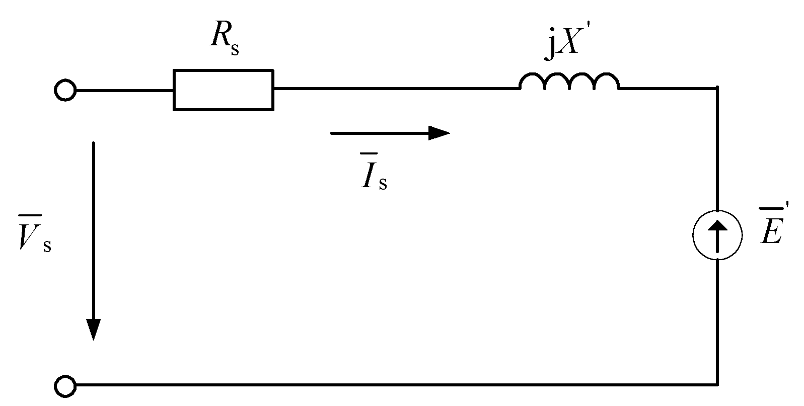
2.1. TS Model of an IM

In modern power systems, motors form a major portion of the loads. Thus it is important to model the induction motors in system analysis. The fifth order (electromagnetic) model and the third order (electromechanical) model are two frequently used IM models in dynamic simulations [21,22,23]. To clearly describe the models, this paper uses V ¯ , E ¯ , and I ¯ to represent phasor voltage, potential and current, V ¯ * , E ¯ * , and I ¯ * to represent their conjugates, and V, E, and I to represent their Root Mean Square (RMS) value.
The fifth order IM model captures the stator and rotor flux dynamics together with the inertia dynamics and hence is adopted in EMT-type simulation packages such as PSCAD/EMTDC and EMTP [24]. Due to its high computation accuracy, it is also used to calibrate the accuracy of other models.
Compared to the rotor dynamics, the stator flux transients are significantly fast; therefore, the fifth order model can be reduced to a third order model to provide a compromise between simplicity and accuracy [25,26]. The third order model is often used in TS-type simulation packages and the differential and algebraic equations (DAEs) governing it are
V ¯ s = E ¯ + ( R s + j X ) I ¯ s
{ d E d d t = 1 T 0 [ E d + ( X X ) I qs ] + s ω s E q d E q d t = 1 T 0 [ E q ( X X ) I ds ] s ω s E d
2 H d s d t = T m T e
where V ¯ s and I ¯ s are the stator terminal voltage and current, respectively; X = Xs + Xm is the rotor open-circuit reactance; X′ = Xs + XrXm/(Xr + Xm) is the transient reactance of the IM; E ¯ is the internal potential behind the transient impedance; Ed′, Eq′, Ids, and Iqs are the d- and q-axis components of E ¯ and I ¯ s , respectively; T0′ = (Xr + Xm)/(ωsRr) is the transient open-circuit time constant characterizing the decay of the rotor transients when the stator is open-circuited; ωs is the synchronous angular velocity of the rotating field; s is the slip; H is the inertia constant of the motor and load; Tm is the load torque; and Te is the electrical torque.
The electrical torque of an IM, as well as the real and reactive powers it draws are calculated by
T e = Re ( E ¯ I ¯ s * )  
{ P e = Re ( V ¯ s I ¯ s * ) Q e = Imag ( V ¯ s I ¯ s * )
The model described above are in a form directly suitable for power system analysis and simulation studies, where rotor flux is represented by the internal potential.
The equivalent circuit corresponding to Equation (1) is shown in Figure 1.
In some cases, we use an alternative representation for the transients of the internal potential, as given in (6).
d E ¯ d t = 1 T 0 [ E ¯ j ( X X ) I ¯ s ] j s ω s E ¯

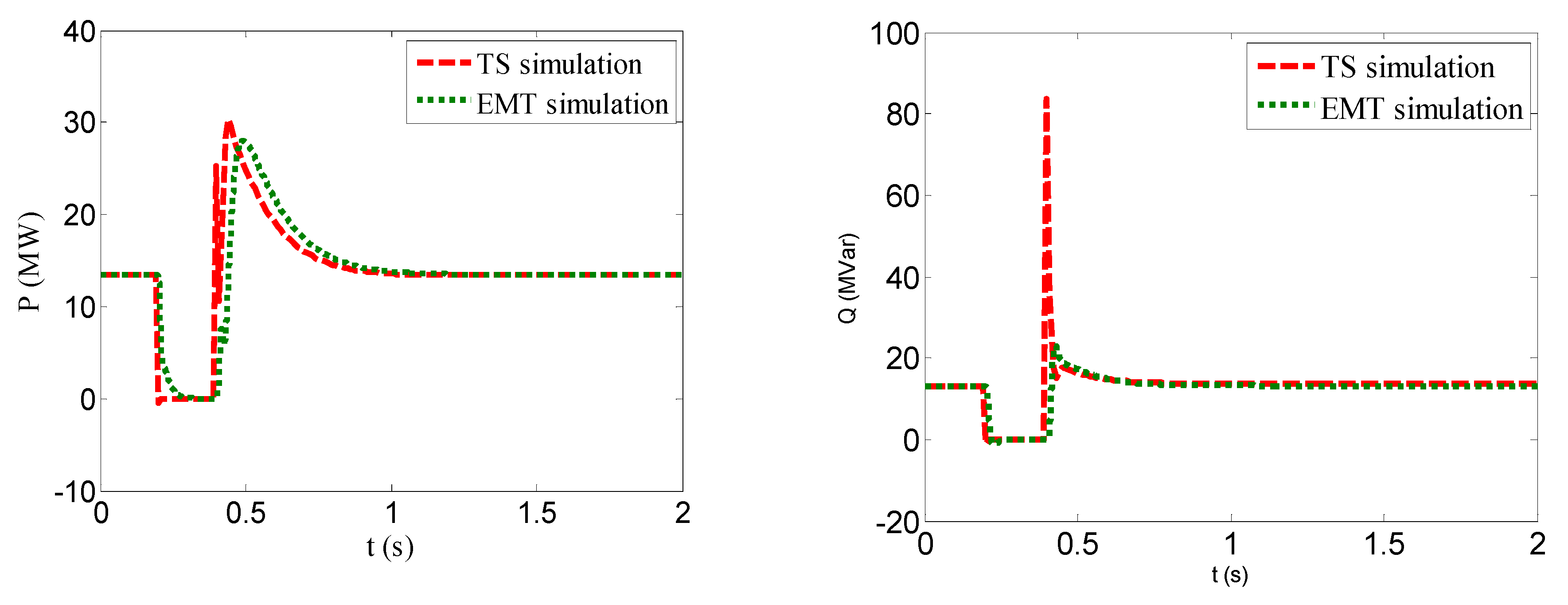
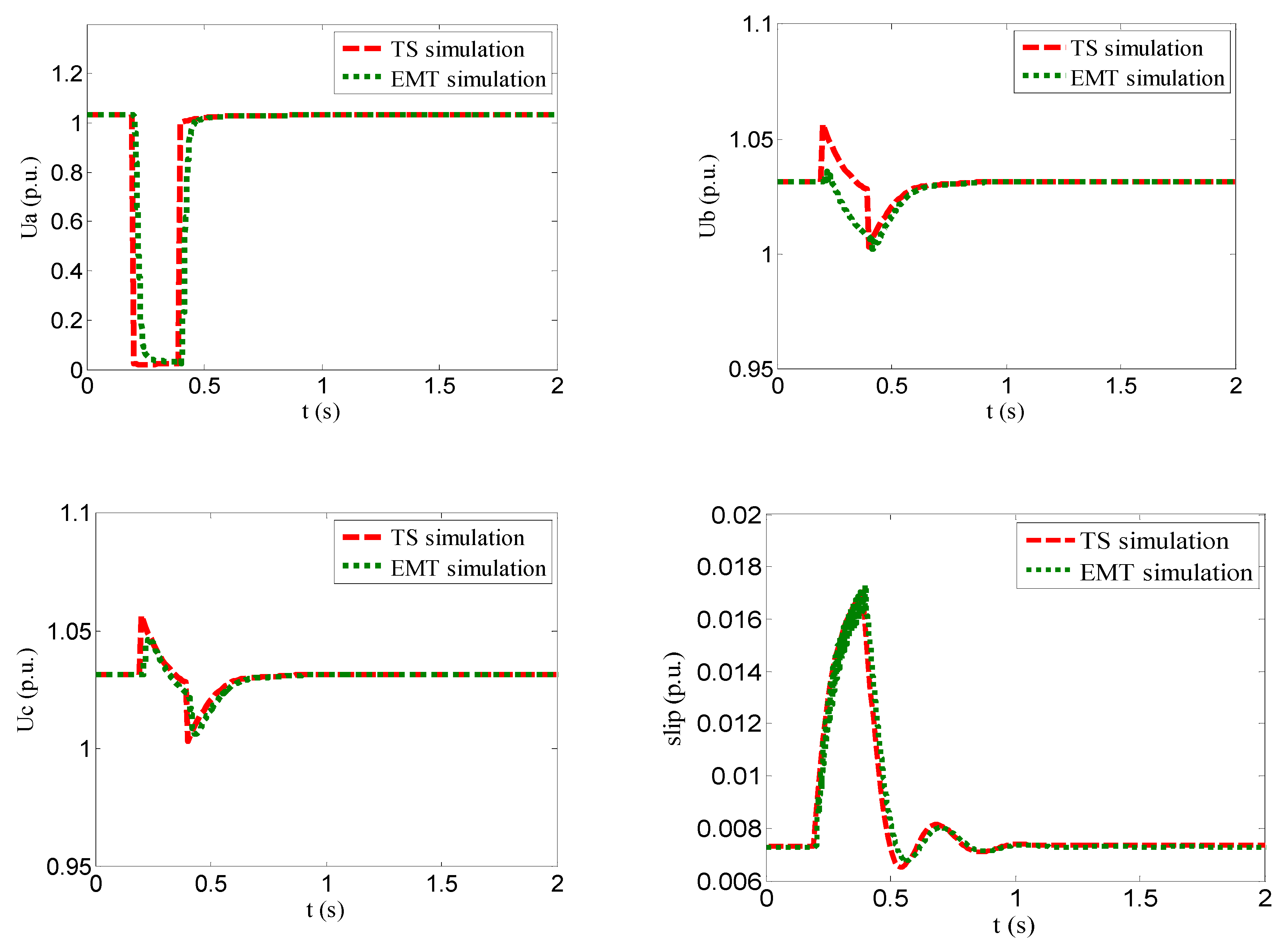
2.2. The Performance of the Traditional TS Model of an IM

The simple power network shown in Figure 2 is used to test the performance of the traditional electromechanical transient model of an IM, where the electric source E ¯ eq feeds the IM through an equivalent system impedance Zeq.
In the following example, we assume Eeq = 115 kV, f = 50 Hz and Zeq = (3.4 + j8.0425) Ω, and the IM is rated at 110 kV, 152.5 A. The typical IM parameters recommended by the Institute of Electrical and Electronics Engineers (IEEE) in [27] are used in this study and listed in Table 1. Without a loss of generality, the load torque of the IMs is assumed to be Tm = m2, where ωm is the rotor speed in p.u.
The faults considered include balanced and unbalanced voltage sags occurring at the power source end at t0 = 0.2 s with the duration 0.2 s. The sag parameters are defined as follows:
Case 1: Balanced voltage sag. During the sag, Eeqadur = Eeqbdur = Eeqcdur = 0 p.u.
Case 2: Unbalanced voltage sag. During the sag, Eeqadur = 0 p.u., Eeqbdur and Eeqcdur remain unchanged.
In Figure 2, we have
E ¯ eq = V s ¯ + ( R eq + j X eq ) I ¯ s
With (7) and the DAEs regarding the IM in (1)–(5), we can obtain the DAEs governing the dynamics of the system under study. Subsequently, both TS simulation and EMT simulation are performed, respectively. In TS simulation implemented in MATLAB, we use the trapezoidal integral rule to convert the dynamic equations to algebraic equations, which are then solved simultaneously with the other algebraic equations to obtain response of the system. The results from EMT simulation program PSCAD/EMTDC is used for comparison. It is worth mentioning that the computed voltages (currents) in EMT simulation are the RMS values provided by the fast Fourier transform to facilitate the comparison. In addition, the computing step size is 10 ms and 100 μs for TS simulation and the PSCAD, respectively.
Figure 3, Figure 4, Figure 5 and Figure 6 show the type-2 and type-5 IM responses during voltage sag in each aforementioned case. It shows that, during the voltage sag, the motor decelerates and the slip increases as a result of the electrical torque drop. After the sag, the speed and P/Q consumptions undergo their transients and restore to their initial values.
In the case of balanced voltage sag, as shown in Figure 3 and Figure 4, it is observed that the traditional TS simulation agrees well with the EMT simulation. While considering that the TS simulation neglects the machine stator transients, the network variables change instantly at the moment of failure, and clearing thus brings some deviation.
In the case of asymmetric voltage sag, the simulation deviation becomes significant. In Figure 5, the TS simulation results of the rotor slip and the active power are reasonable, but the deviations of the reactive power and the stator voltages is significant. In Figure 6, except for the Q and V dynamics, predictions of slip and active power are also unacceptable. The results indicate that in the case of asymmetric fault, IM dynamics obtained by TS simulation are not satisfactory. The reason is that only the positive-sequence components are considered in TS simulation, but, in asymmetric faults, the negative-sequence components have a considerable contribution. Therefore, it is necessary to consider the influence of the negative-sequence components.

3. Integrated TS Model of an IM Considering Negative-Sequence Components

When subject to unbalanced disturbances, both positive- and negative-sequence voltages will act on the response of an IM. The symmetrical component method can be used to analyze their effects.
In this section, before deriving the negative-sequence equations of an IM, we will review the derivation process of the traditional electromechanical model of an IM first. Then, the integrated model, including the positive- and negative-sequence equations, will be formulated.

3.1. Derivation Process of the Traditional TS Model of an IM

As described in Section 2.1, Equations (1)–(5) constitute the electromechanical transient model of an IM, among which the stator voltage Equation (1) and rotor flux Equation (2) are especially noteworthy. Their derivation is summarized as follows according to [2].
Step 1: Write the voltage and flux linkage equations for the stator and rotor in their own reference frame.
Step 2: Apply the d-q transformation to obtain the voltage and flux linkage equations in the d-q reference frame, which rotates at synchronous speed in the direction of rotation; the q-axis is 90° ahead of the d-axis.
Step 3: In the d-q reference frame, substitute the stator and rotor flux equations into the voltage equations and rearrange them to get the stator voltage Equation (1) and the rotor flux dynamics (2).
The equations regarding the negative-sequence components can be derived using the similar procedures. Note that when counting in the influence of the negative-sequence components, the rotor acceleration Equation (3) remains unchanged.

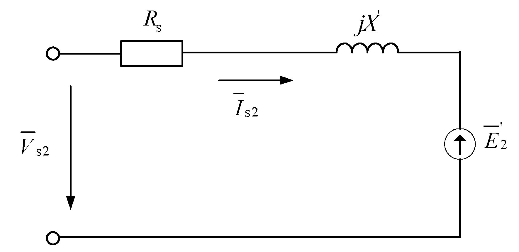
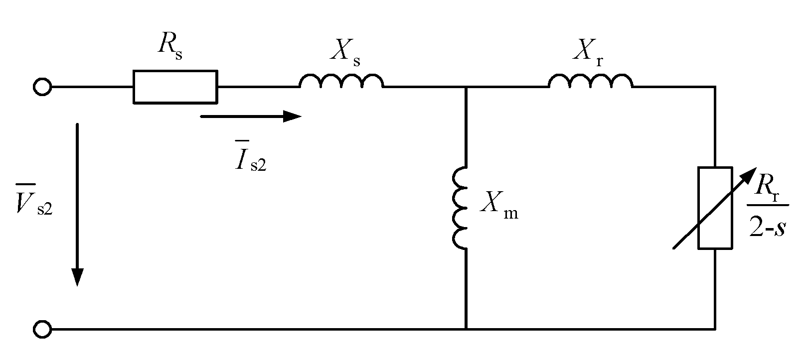
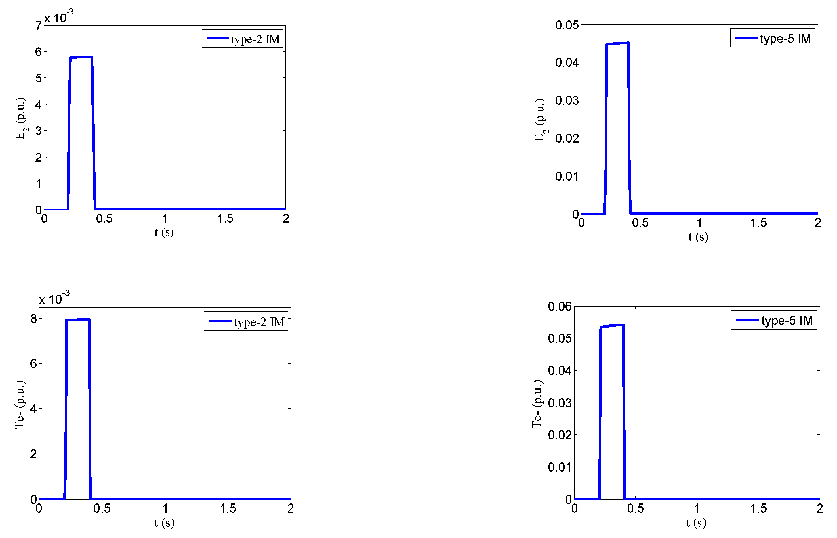
3.2. Negative-Sequence TS Model of an IM

With negative-sequence voltages presence at the IM terminal, negative-sequence stator currents appear, giving rise to the negative-sequence rotating field which rotates against the rotor at the synchronous speed. In this case, the stator and rotor voltage equations are:
{ v a = p ψ a + R s i a v b = p ψ b + R s i b v c = p ψ c + R s i c
{ v A = p ψ A + R r i A v B = p ψ B + R r i B v C = p ψ C + R r i C
In (8) and (9), a, b, and c denote the stator three-phase winding; A, B, and C denote the rotor three-phase winding; v and i represent the voltages and currents of the windings denoted by the subscript; Ψ represents the flux linking the winding; and p represents the differential operator d/dt. Note that when negative-sequence voltages are applied at the stator terminals, the stator and rotor voltage equations remain consistent with that in the positive-sequence equations in the forward rotating d-q reference frame in [2].
The flux linkage in the stator phase a winding at any instant is
ψ a = L aa i a + L ab ( i b + i c ) +      L aA [ i A cos θ + i B cos ( θ 120 ) + i C cos ( θ + 120 ) ]
where Laa is the self-inductance of stator windings, Lab the mutual inductance between stator windings, and LaA is the maximum value of mutual inductance between stator and rotor windings. θ is defined as the angle by which the axis of phase A rotor winding leads the axis of phase a stator winding in the direction of rotation. Similar expressions apply to Ψb and Ψc.
The flux linkage in the rotor phase A winding is given by
ψ A = L AA i A + L AB ( i B + i C ) +      L aA [ i a cos θ + i b cos ( θ + 120 ) + i c   cos ( θ 120 ) ]
Similar expressions apply to ΨB and ΨC.
With no neural currents due to winding connections and let
{ L ss =   L aa L ab L rr = L AA L AB
The expressions for flux linkage in the stator and rotor are written as:
[ ψ a ψ b ψ c ] = L ss [ i a i b i c ] + L aA [ cos θ cos ( θ 120 ) cos ( θ + 120 ) cos ( θ + 120 ) cos θ cos ( θ 120 ) cos ( θ 120 ) cos ( θ + 120 ) cos θ ] [ i A i B i C ]
[ ψ A ψ B ψ C ] = L rr [ i A i B i C ] + L aA [ cos θ cos ( θ + 120 ) cos ( θ 120 ) cos ( θ 120 ) cos θ cos ( θ + 120 ) cos ( θ + 120 ) cos ( θ 120 ) cos θ ] [ i a i b i c ]
Note that with negative-sequence voltage presence at the stator terminal, the stator and rotor flux equations have changed compared to those in [2].
To transform phase variables in (8), (9), (13), and (14) into components along the reverse rotating axes, the d-q transformations used in this case are:
[ A ds A qs ] = 2 3 [ cos ( θ r + θ ) cos ( θ r + θ + 120 ) cos ( θ r + θ 120 ) sin ( θ r + θ ) sin ( θ r + θ + 120 ) sin ( θ r + θ 120 ) ] [ A a A b A c ]
[ A dr A qr ] = 2 3 [ cos θ r cos ( θ r + 120 ) cos ( θ r 120 ) sin θ r sin ( θ r + 120 ) sin ( θ r 120 ) ] [ A A A B A C ]
In (15) and (16), θr is the angle by which d- axis leads phase A axis of the rotor. Aa, Ab, and Ac represent negative-sequence stator phase components, and Ads and Aqs are their corresponding d-q axes components. AA, AB, and AC represent negative-sequence rotor phase components, and Adr and Aqr are their corresponding d-q axes components. The transformations apply to currents, voltages, and flux linkages.
Their inverse transformations are:
[ A a A b A c ] = [ cos ( θ r + θ ) sin ( θ r + θ ) cos ( θ r + θ + 120 ) sin ( θ r + θ + 120 ) cos ( θ r + θ 120 ) sin ( θ r + θ 120 ) ] [ A ds A qs ]
[ A A A B A C ] = [ cos θ r sin θ r cos ( θ r + 120 ) sin ( θ r + 120 ) cos ( θ r 120 ) sin ( θ r 120 ) ] [ A dr A qr ]
Note that the d-q transformations and their inverse transformations defined by Equations (15)–(18) are also different from those in [2].
After the d-q transformation, the voltage and flux linkage equations for the stator and rotor in the d-q reference frame are:
{ v ds = R s i ds ω s ψ qs + p ψ ds v qs = R s i qs + ω s ψ ds + p ψ qs
{ v dr = R r i dr ( p θ r ) ψ qr + p ψ dr v qr = R r i qr + ( p θ r ) ψ dr + p ψ qr
{ ψ ds = L ss i ds +   L m i dr ψ qs = L ss i qs +   L m i qr
{ ψ dr = L rr i dr +   L m i ds ψ qr = L rr i qr +   L m i qs
where Lm = 3/2 LaA. Note that Equations (19)–(22) are identical to the positive-sequence voltage and flux equations in the forward rotating d-q reference frame in [2]. However, in the reverse rotating case, the term r is (2−s)ωs instead of s.
Then, by neglecting the stator transients ds and qs in (19), letting the rotor windings shorted, and substituting the stator and rotor flux linkage equations into the voltage equations, the derived stator voltage equation expressed in phasor form is:
V ¯ s 2 = E ¯ 2   +   ( R s + j X ) I ¯ s 2
where V ¯ s 2 , I ¯ s 2 , and E ¯ 2 are the negative-sequence stator terminal voltage, current, and internal potential, respectively. The corresponding equivalent circuit is shown in Figure 7, which is similar to Figure 1.
The equations describing the rotor circuit dynamics are:
{ d E 2 d d t = 1 T 0 [ E 2 d + ( X X ) I qs 2 ] +   ( 2 s ) ω s E 2 q d E 2 q d t = 1 T 0 [ E 2 q ( X X ) I ds 2 ] ( 2 s ) ω s E 2 d
where E2d′ and E2q′, Ids2, and Iqs2 are the d- and q-axis components of E ¯ 2 and I ¯ s 2 , respectively.
Equation (24) may also be written as:
d E ¯ 2 d t = 1 T 0 [ E ¯ 2 j ( X X ) I ¯ s 2 ] j ( 2 s ) ω s E ¯ 2
Equation (23) describes the relations between the negative-sequence terminal voltage, current, and internal potential, and (24) gives the dynamics of the negative-sequence internal potential. It can be found that (23) and (24) are very similar to (1) and (2), with the differences in that the negative-sequence components are denoted by the subscript 2, and the s in (2) is replaced by (2–s)ωs in (24).

3.3. Integrated TS Model of an IM Including Positive- and Negative-Sequence Components

With the negative-sequence equations included, the machine electrical torque and power consumptions in (4) and (5) are corrected into:
T e = T e + +   T e   =   Re ( E ¯ I ¯ s * E ¯ 2 I ¯ s 2 * )
{ P e = P e + +   P e   =   Re ( V ¯ s I ¯ s *   +   V ¯ s 2 I ¯ s 2 * ) Q e = Q e + +   Q e   =   Imag ( V ¯ s I ¯ s * V ¯ s 2 I ¯ s 2 * )
where the superscripts + and – represent positive- and negative-sequence components, respectively.
Equations (1)–(3), (23), (24), (26) and (27) constitute the integrated electromechanical transient model of an IM in stability studies considering the negative-sequence components. In the following, we refer to them as the Integrated TS (ITS) model of an IM.
During an asymmetric voltage sag, the three-phase potentials of the electric source are decomposed into positive-, negative-, and zero-sequence components as:
[ E ¯ eq 1 E ¯ eq 2 E ¯ eq 0 ] = 1 3 [ 1 a a 2 1 a 2 a 1 1 1 ] [ E ¯ eqa E ¯ eqb E ¯ eqc ]
where a = 1 120 is a complex operator, the subscripts a, b, and c denote the phase components, while 1, 2, and 0 represent the positive-, negative-, and zero-sequence components, respectively. Then we have the negative-sequence network equation:
E ¯ eq 2 = V ¯ s 2 + ( R eq + j X eq ) I ¯ s 2
The overall system model for the studied power network shown in Figure 2 includes Equations (1)–(3), (7), (23), (24), (26), (27) and (29), where Equations (1)–(3), (23), (24), (26) and (27) are the ITS model of the IM; (7) and (29) are the network equations.

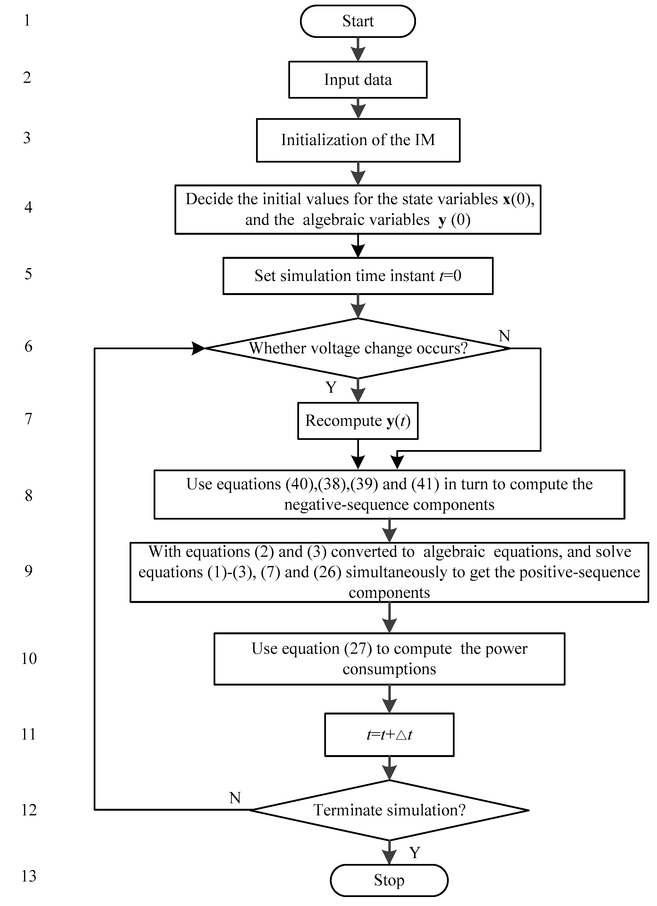
4. Solution of the Integrated Model of an IM

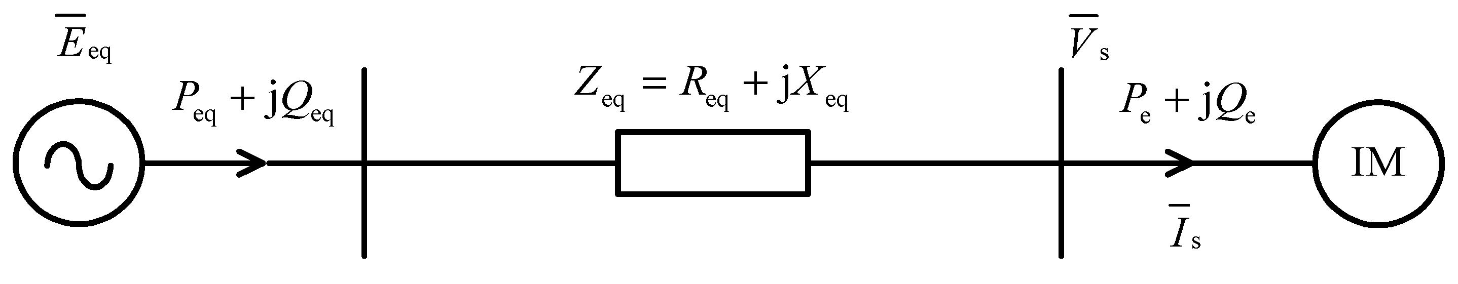
4.1. A Regular Solution Method

Equations (24) and its phasor form (25) are developed in the reverse rotating d-q reference frame. To solve it, we substitute (23) into (25) and get:
d E ¯ 2 d t = 1 T 0 [ E ¯ 2 j ( X X ) V ¯ s 2 E ¯ 2 ( R s + j X ) ] j ( 2 s ) ω s E ¯ 2
(30) can be rearranged as
d E ¯ 2 d t = j ( X X ) T 0 ( R s + j X ) V ¯ s 2 [ 1 T 0 + j ( X X ) T 0 ( R s + j X ) + j ( 2 s ) ω s ] E ¯ 2
Let
{ K E 2 = 1 T 0 + j ( X X ) T 0 ( R s + j X ) + j ( 2 s ) ω s B E = j ( X X ) T 0 ( R s + j X )
We get
d E ¯ 2 d t = K E 2 E ¯ 2 + B E V ¯ s 2
(33) is a first-order non-homogeneous linear differential equation and its analytical solution is
E ¯ 2 dur ( t ) = B E K E 2 V ¯ s 2 + ( E ¯ 20 B E K E 2 V ¯ s 2 ) e K E 2 ( t t 0 )
where t0 is the moment of failure, E ¯ 2 dur ( t ) is the negative-sequence transient potential during voltage sag, and its initial value E ¯ 20 is zero.
After the sag, only positive-sequence voltage presents at the IM bus, while the negative-sequence internal potential will decay to zero and is calculated by:
E ¯ 2 after ( t ) = B E K E 2 V ¯ s 2 + ( E ¯ 21 B E K E 2 V ¯ s 2 ) e K E 2 ( t t 1 )
where t1 is the moment of clearing, E ¯ 2 after ( t ) is the negative-sequence transient potential after voltage sag, and E ¯ 21 is the negative-sequence transient potential at time t1.
Equations (34) and (35) give the analytical solution of E ¯ 2 during and after the sag. In the ITS model, we use E ¯ 1 solved by the trapezoidal integration rules, and E ¯ 2 calculated by (34) or (35) to synthesize the IM dynamics under asymmetric faults. Note that the ITS model adds two differential equations to consider the negative-sequence components to improve simulation accuracy but brings heavier computation burden. To make a trade-off between accuracy and computation time, in the following we further propose a practical method which approximately treat the negative-sequence components.

4.2. Approximate Treatment of the Negative-Sequence Components

Figure 8 gives the negative-sequence steady-state equivalent circuit of an IM whose input impedance is:
Z in 2 = ( R s + j X s ) + j X m ( R r 2 s + j X r ) R r 2 s + j ( X m + X r )
Generally, the initial slip of an IM is small, and, under an asymmetric voltage sag, the variation in slip will not be large. Then we consider the slip as zero and have:
Z in 2 ( R s + j X s ) + j X m ( R r 2 + j X r ) R r 2 + j ( X m + X r )
Equation (37) approximates the equivalent impedance of an IM to a constant impedance during an asymmetrical fault. Thus, with negative-sequence stator voltage V ¯ s 2 presenting at the terminal, the final value of I ¯ s 2 can be estimated by:
I ¯ s 2 = V ¯ s 2 Z in 2
Since Zin2 is small, Is2 is usually large.
According to Figure 7, and considering Equation (38), we have
E ¯ 2 = V ¯ s 2 ( R s + j X ) I ¯ s 2 R V ¯ s 2
where R = 1 ( R s + j X ) / Z in 2 is a complex constant. The magnitude of R measures the ratio of the negative-sequence internal potential to the terminal voltage and is termed as negative-sequence internal potential coefficient here.
Table 2 lists the defined coefficients and the transient open-circuit time constant T0′ of the seven sets of typical IMs recommended by IEEE in [27]. It is seen that the magnitudes of R are generally small, but that of the type-5 and type-7 IM are relatively large.
In power systems, the maximum value of the IM negative-sequence stator voltage Vs2 is approximately 1/3 p.u.; correspondingly, the negative-sequence internal potential E2′ will not exceed 0.05 p.u. Further considering that the time constant corresponding to E2′ is large, the IM negative-sequence components, e.g., E2′, Is2, and T e , will reach their final value very quickly in the dynamics. In view of this, during an asymmetric fault, we may ignore their transients and assume that they achieve their final values instantly, which is equivalent to replacing the IM with Zin2 in the power network shown in Figure 2 during the sag. Thus, V ¯ s 2 can be predicted by:
V ¯ s 2 = E ¯ eq 2 Z in 2 Z in 2 + Z eq
Then I ¯ s 2 , E ¯ 2 , and T e can be estimated by (38), (39), and (41), respectively.
T e = Re ( E ¯ 2 I ¯ s 2 * )
Similarly, after the sag, all the negative-sequence components will revert to zero quickly, and we may assume that they restore to zero instantly. In this way, we can fast predict the negative-sequence components during and after the sag.
Figure 9 shows the flow chart of the proposed practical method, which uses the traditional TS simulation and the approximate treatment to deal with the positive- and negative-sequence equations, respectively, to obtain the transient response of an IM. There are thirteen steps in Figure 9, with steps 8, 9, and 10 being the most important. In step 8, the negative-sequence components are estimated by using Equations (40), (38), (39), and (41) in turn, and the obtained negative-sequence electrical torque is then used to compute the rotor slip in step 9. Finally, in step 10, active and reactive power consumptions of the IM are obtained.
The ITS and simplified models proposed in Section 4.1 and Section 4.2 are both improved TS models. Therefore, their simulation step sizes are also set as 10 ms in this study.

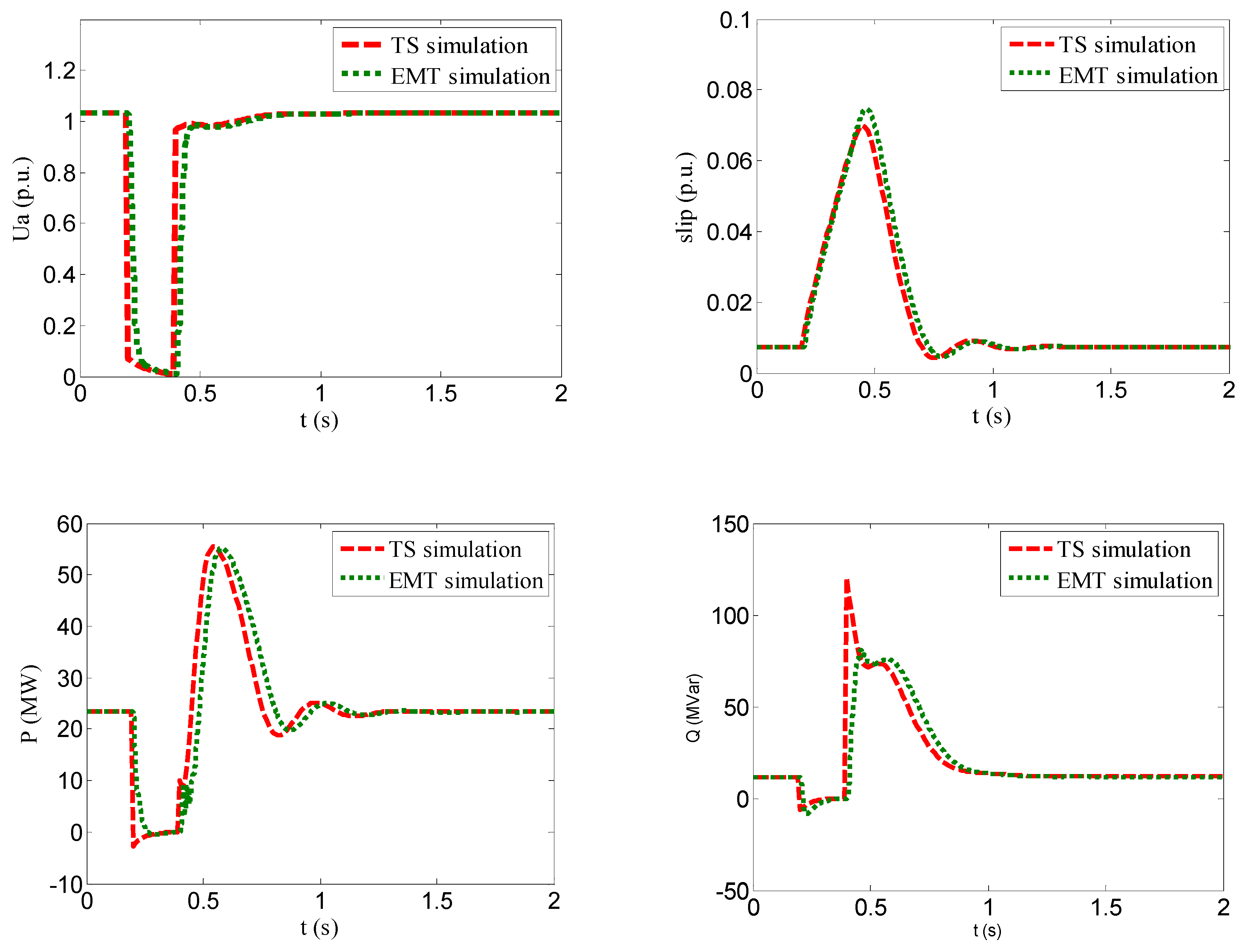
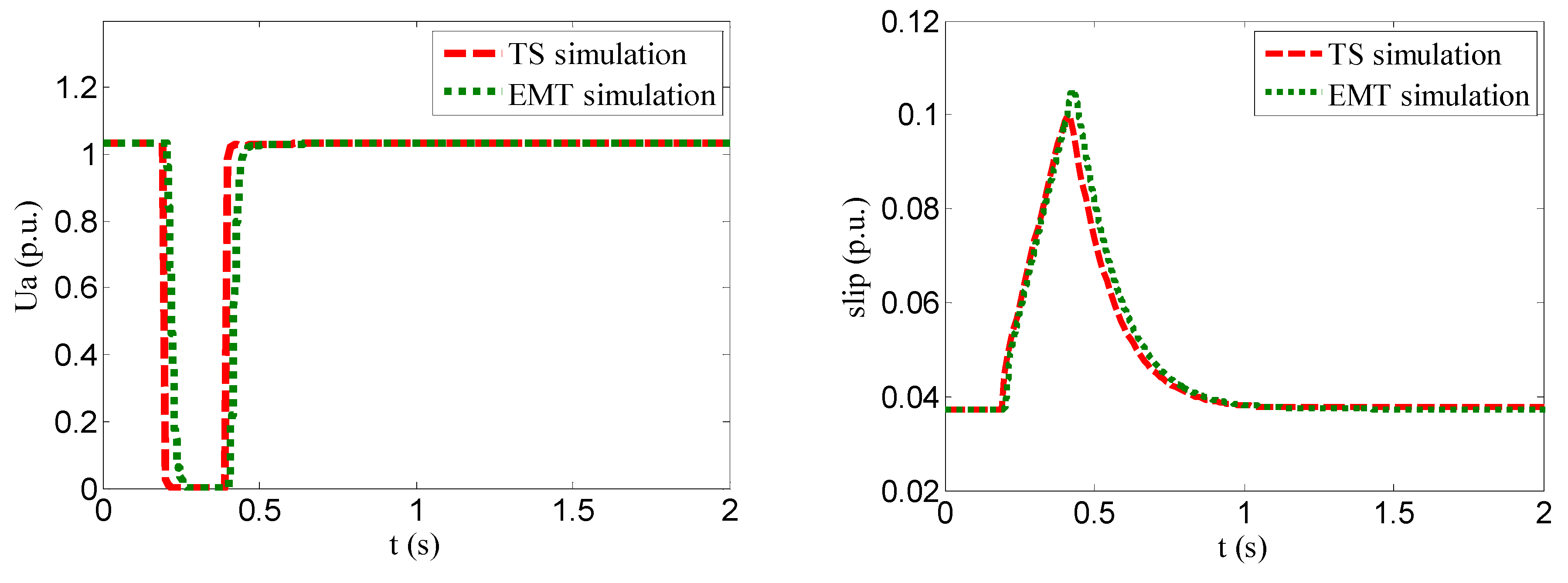
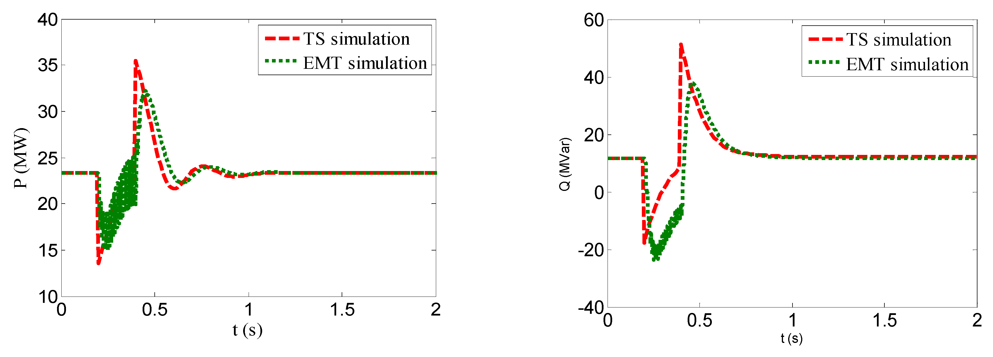
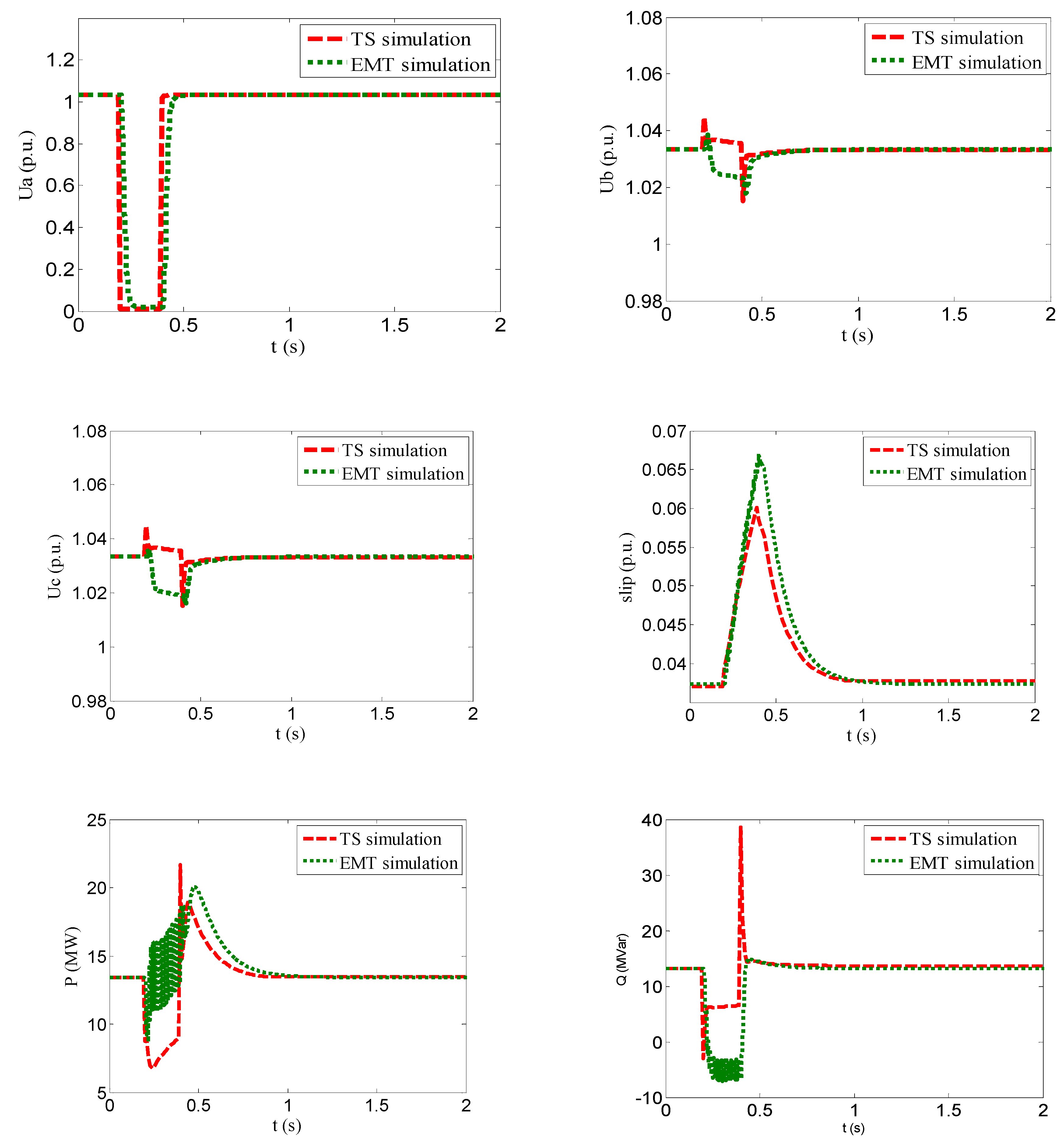
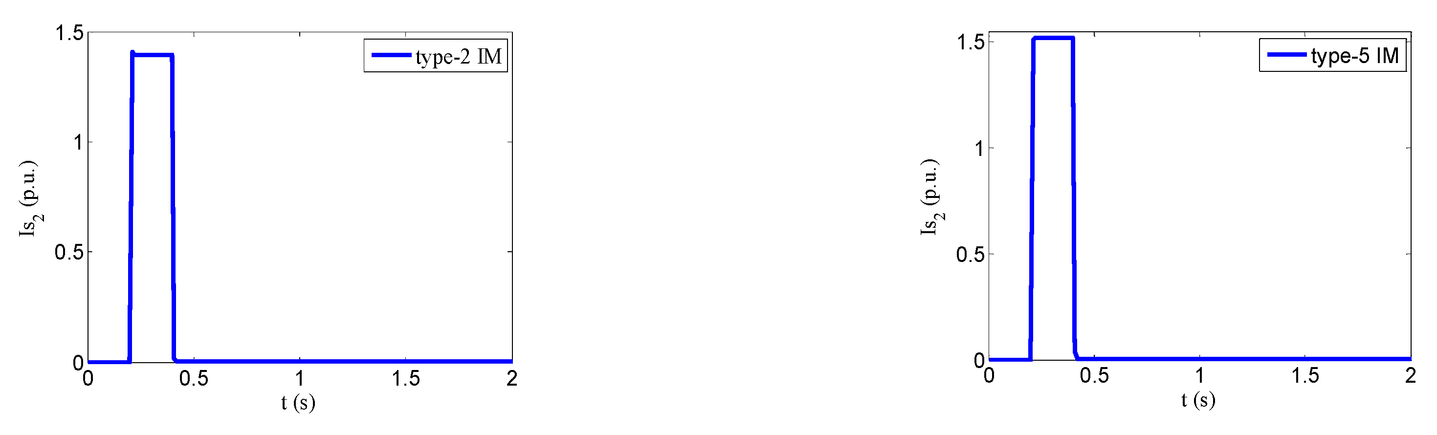
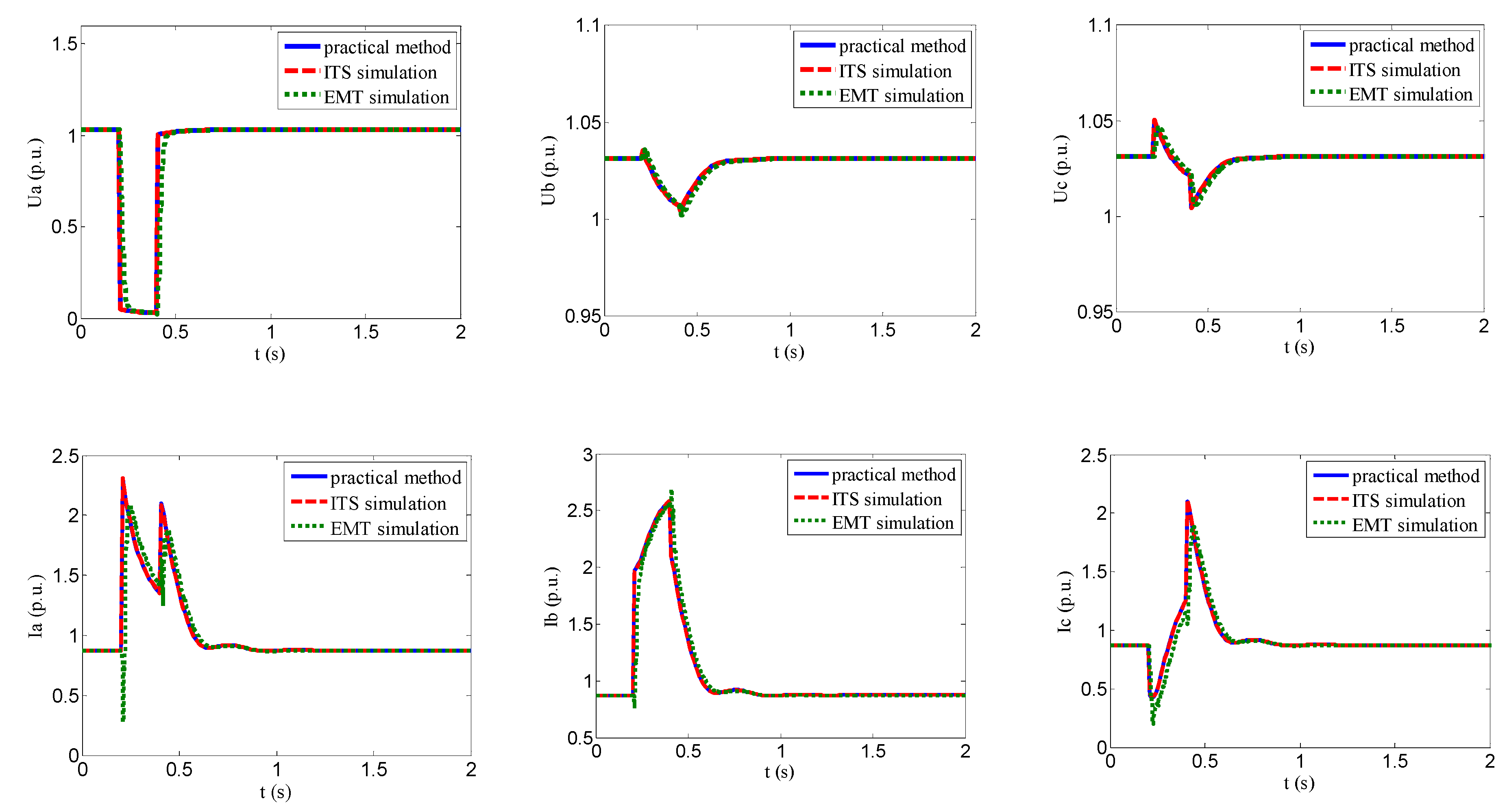
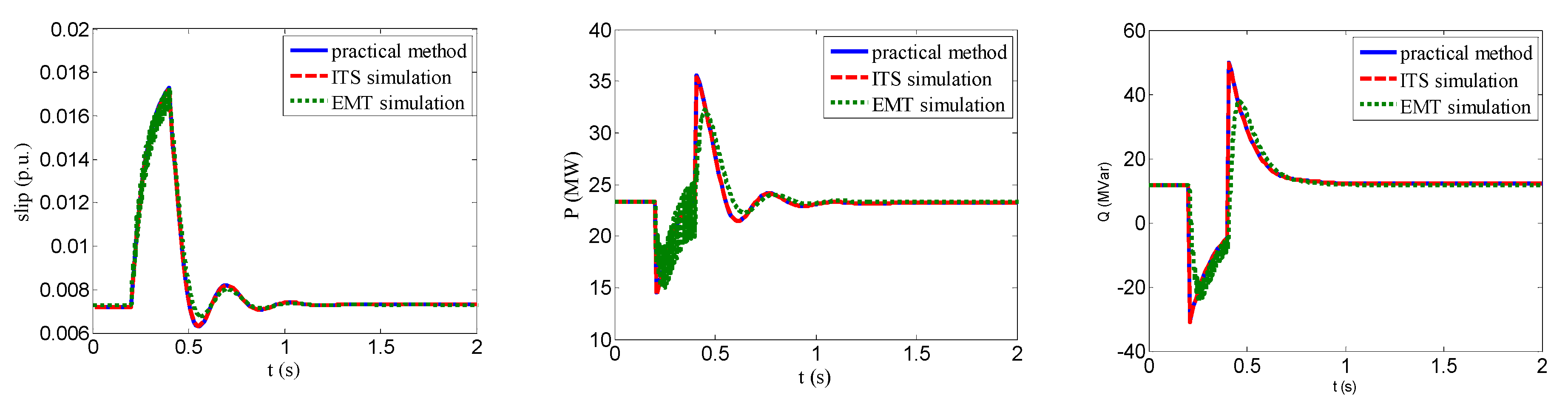
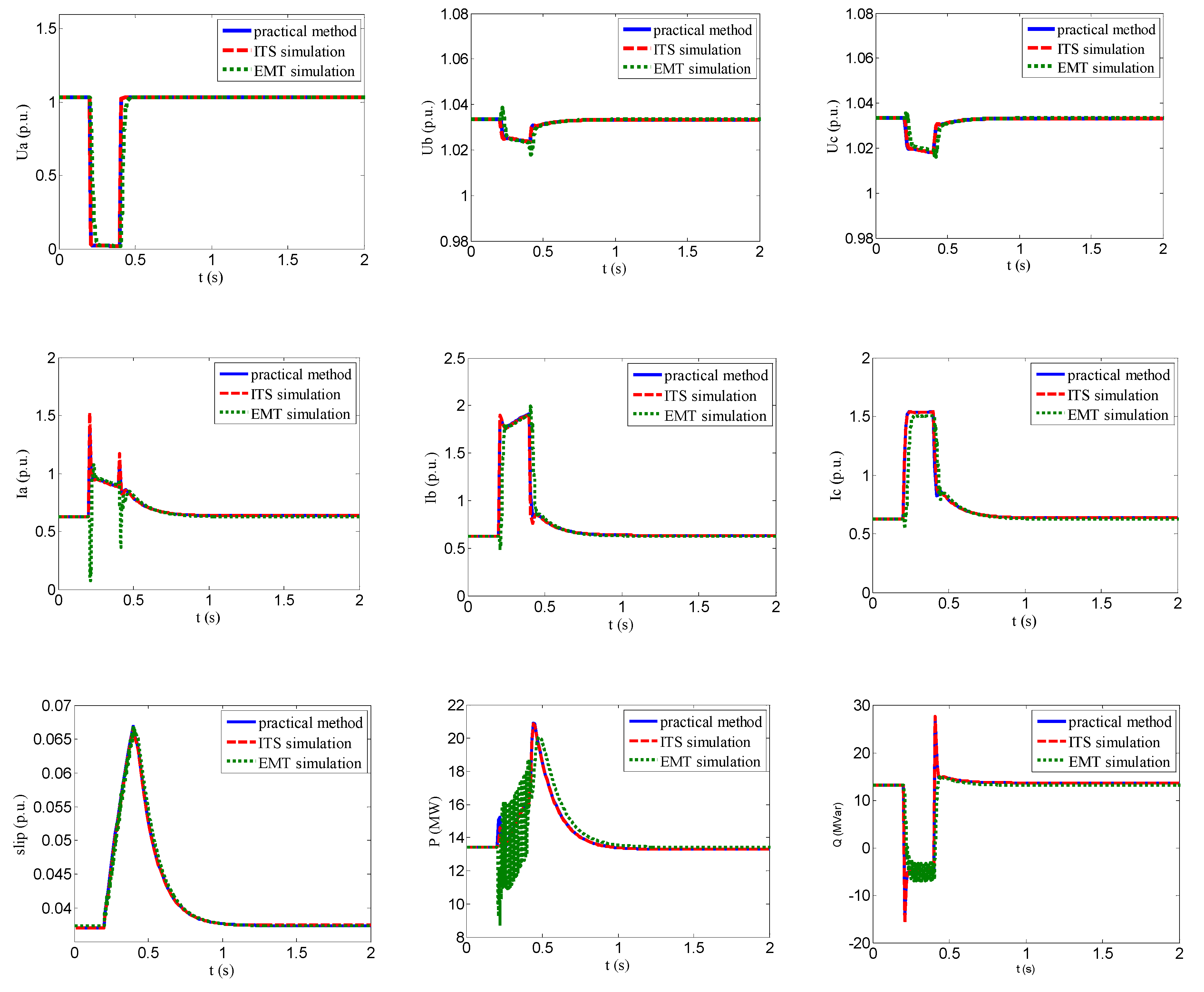
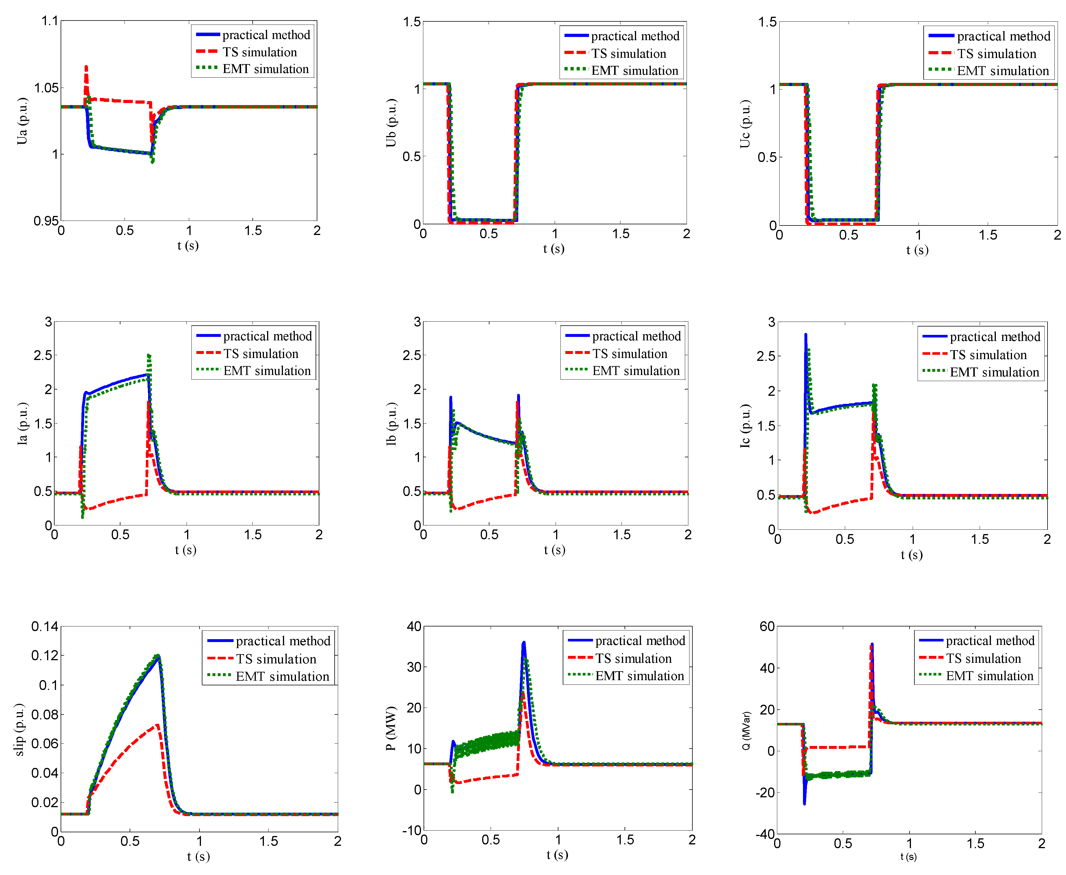
4.3. Verification and Discussion

Figure 10 shows the Is2, E2′, and T e dynamics obtained through the ITS model with the type-2 and type-5 IM under the asymmetric voltage sag defined in Section 2.2. It is seen the waveforms of all negative-sequence components look like square waves. The negative-sequence stator current Is2 of type-2 and type-5 IM are large, and the E2′ and T e of type-5 IM are larger than that of type-2 IM, which justifies the analysis in Section 4.2.
Figure 11 and Figure 12 compare the IM responses obtained by the practical method (solid line), the ITS model (dashed line) implemented in MATLAB, and the EMT simulation (dot line) under the aforementioned unbalanced voltage sag. It is seen both the practical method and the ITS simulation agree well with the EMT simulation, which validates the correctness of the proposed model and the computation method. The observed difference in powers is attributed to the fact that, during an asymmetric fault, the instantaneous active and reactive powers an IM draws include doubled frequency components. The EMT simulation uses very small step size and, hence, captures the oscillatory response; while in TS simulation, the phasor modelling technology is used and reflects only the averages.
From the simulation results in Figure 11 and Figure 12, we can find that the ITS model and the practical method consider the influence of the negative-sequence components and, thus, provide satisfactory results. Note that the practical method only adds several algebraic equations considering the negative-sequence components during faults and therefore require a little more computation effort than that of the traditional TS model, i.e., achieving a trade-off between accuracy and computation time. In the test system, the time consumptions of the TS simulation, the practical method and the ITS model are 0.62 s, 0.621 s, and 1.18 s, respectively, with a Core i7-6700 CPU and 16 GB RAM computing platform, which means the ITS model requires approximate twice the time of the TS simulation; the practical method shares almost the same computation efficiency as the TS simulation.
According to the simulation results in Figure 5 and Figure 6, it can be observed that under asymmetric fault, negative-sequence stator currents Is2 would be considerable but is ignored in TS simulation. As a result, the predictions of V ¯ s 2 in Equation (29) and, accordingly, the machine phase voltages (Ua, Ub, Uc) are rough. In addition, for type-5 IM, a relatively large E2′ brings a relatively large negative-sequence electrical torque T e . Since T e is neglected in TS simulation, the calculation of the active power and slip is of poor accuracy.
As we all know, the slip of an IM is small; hence, very low negative-sequence voltages will contribute to considerable negative-sequence currents Is2 on the motor. The traditional TS simulation ignores Is2 so that the computational error under asymmetric faults is significant. Taking the active power as an example, since the value of Pe may be greater than Pe+, when Pe is omitted, the relative error may even be higher than 100%. While when the negative-sequence is properly modelled in the proposed practical method, the error is almost negligible. The above results validate that it is of great significance to include the negative-sequence components in TS simulation.
We have tested other types of IMs recommended by [27] under various asymmetric voltage sags with different durations using the practical method. A similar agreement between responses obtained with MATLAB and PSCAD is observed. Figure 13 illustrates the response of the type-7 IM when Eeqb and Eeqc drops to zero for 0.5 s in the test system. It is observed the practical method still gives satisfactory results even when a very serious asymmetrical fault occurs, whereas the traditional TS simulation gives poor prediction.
The proposed practical simulation method can be also applied to multi-machine power systems under asymmetric faults using the following steps. Firstly, replace the IMs with their approximate negative-sequence steady-state equivalent impedances during the fault to form the new negative-sequence network. Subsequently, combine the effective negative- and zero-sequence impedance calculated at the fault location with the positive-sequence network according to the type of the unbalance fault. Then, solve the overall network equations to obtain the negative-sequence terminal voltages of the IMs. Finally, the other negative-sequence components, such as I ¯ s 2 , E ¯ 2 , and T e , can be accordingly calculated.

5. Conclusions

Motors consume 60 to 70% of the total energy supplied by a power system. The dynamics attributable to motors are usually the most significant aspects of dynamic characteristics of system loads. In this work, modeling and simulation of induction motor loads in power system stability studies considering the influence of the negative-sequence components are explored. A practical method to calculate the transient response of an IM is proposed. The method can well predict the IM behavior subject to asymmetric faults. Compared with the existing TS simulation, it adds a little computational burden yet achieves much better simulation accuracy.

Author Contributions

X.M. proposed the original idea, conceived and designed the experiments, analyzed and verified the results, and wrote the full manuscript. J.C. wrote the program and performed the experiments.

Acknowledgments

This research was funded by Natural Science Foundation of Guangdong Province, China [2014A030313509].

Conflicts of Interest

The authors declare no conflict of interest.

References

  1. Larik, R.; Mustafa, M.W.; Aman, M.; Jumani, T.; Sajid, S.; Panjwani, M. An improved algorithm for optimal load shedding in power systems. Energies 2018, 11, 1808. [Google Scholar] [CrossRef]
  2. Kundur, P. Power System Stability and Control; McGraw-Hill: New York, NY, USA, 1994; pp. 271–305. [Google Scholar]
  3. Modarresi, J.; Gholipour, E.; Khodabakhshian, A. A comprehensive review of the voltage stability indices. Renew. Sustain. Energy Rev. 2016, 63, 1–12. [Google Scholar] [CrossRef]
  4. Oluic, M.; Ghandhari, M.; Berggren, B. Methodology for rotor angle transient stability assessment in parameter space. IEEE Trans. Power Syst. 2017, 32, 1202–1211. [Google Scholar]
  5. Lin, Z.; Zhao, Y.; Liu, S.; Wen, F.; Ding, Y.; Yang, L.; Han, C.; Zhou, H.; Wu, H. A new indicator of transient stability for controlled islanding of power systems: Critical islanding time. Energies 2018, 11, 2975. [Google Scholar] [CrossRef]
  6. Chen, Z.; Han, X.; Fan, C.; Zheng, T.; Mei, S. A two-stage feature selection method for power system transient stability status prediction. Energies 2019, 12, 689. [Google Scholar] [CrossRef]
  7. Dai, W.; Yu, J.; Liu, X.; Li, W. Two-tier static equivalent method of active distribution networks considering sensitivity, power loss and static load characteristics. Int. J. Electr. Power Energy Syst. 2018, 100, 193–200. [Google Scholar] [CrossRef]
  8. Asres, M.W.; Girmay, A.A.; Camarda, C.; Tesfamariam, G.T. Non-intrusive load composition estimation from aggregate ZIP load models using machine learning. Int. J. Electr. Power Energy Syst. 2019, 105, 191–200. [Google Scholar] [CrossRef]
  9. Li, H.; Chen, Q.; Fu, C.; Yu, Z.; Shi, D.; Wang, Z. Bayesian estimation on load model coefficients of ZIP and induction motor model. Energies 2019, 12, 547. [Google Scholar] [CrossRef]
  10. Ge, H.; Guo, Q.; Sun, H.; Wang, B.; Zhang, B.; Wu, W. A load fluctuation characteristic index and its application to pilot node selection. Energies 2014, 7, 115–129. [Google Scholar] [CrossRef]
  11. Liu, J.; Xu, Y.; Dong, Z.Y.; Wong, K.P. Retirement-driven dynamic VAR planning for voltage stability enhancement of power systems with high-level wind power. IEEE Trans. Power Syst. 2018, 33, 2282–2291. [Google Scholar] [CrossRef]
  12. Guan, L.; Wu, L.; Li, F.; Zhao, Q. Heuristic planning for dynamic VAR compensation using zoning approach. IET Gener. Transm. Distrib. 2017, 11, 2852–2861. [Google Scholar] [CrossRef]
  13. Siemens, P.T.I. PSSE User’s Manual; Version 33.4; Siemens Industry, Inc. Siemens Power Technologies International: Schenectady, NY, USA, 2013. [Google Scholar]
  14. Tools, D.S.A. TSAT Model Manual; Version 8.0; Powertech Labs Inc.: Surrey, BC, Canada, 2011. [Google Scholar]
  15. Tang, Y.; Bo, G.Q.; Hou, J.X. PSD-BPA Transient Stability Program User Manual; Chinese Version 4.15; China Electric Power Science Research Institute: Beijing, China, 2007. [Google Scholar]
  16. Pedra, J.; Candela, I.; Sainz, L. Modelling of squirrel-cage induction motors for electromagnetic transient programs. IET Electr. Power Appl. 2009, 3, 111–122. [Google Scholar] [CrossRef]
  17. Al-Jufout, S.A. Modeling of the cage induction motor for symmetrical and asymmetrical modes of operation. Comput. Electr. Eng. 2003, 29, 851–860. [Google Scholar] [CrossRef]
  18. Ikeda, M.; Hiyama, T. Simulation studies of the transients of squirrel-cage induction motors. IEEE Trans. Energy Convers. 2007, 22, 233–239. [Google Scholar] [CrossRef]
  19. Su, H.T.; Chan, K.W.; Snider, L.A. Parallel interaction protocol for electromagnetic and electromechanical hybrid simulation. IEE Proc. Gener. Transm. Distrib. 2005, 152, 406–414. [Google Scholar] [CrossRef]
  20. Van der Meer, A.A.; Gibescu, M.; van der Meijden, M.A.; Kling, W.L.; Ferreira, J.A. Advanced Hybrid Transient Stability and EMT Simulation for VSC-HVDC Systems. IEEE Trans. Power Deliver. 2015, 30, 1057–1066. [Google Scholar] [CrossRef]
  21. Ahmed-Zaid, S.; Taleb, M. Structural modeling of small and large induction machines using integral manifolds. IEEE Trans. Energy Convers. 1991, 6, 529–535. [Google Scholar] [CrossRef]
  22. Martín, H.; de la Hoz, J.; Monjo, L.; Pedra, J. Study of Reduced-order Models of Squirrel-cage Induction Motors. Electr. Power Compon. Syst. 2011, 39, 1542–1562. [Google Scholar] [CrossRef]
  23. Thiringer, T.; Luomi, J. Comparison of reduced-order dynamic models of induction machines. IEEE Trans. Power Syst. 2001, 16, 119–126. [Google Scholar] [CrossRef]
  24. Borghetti, A.; Caldon, R.; Mari, A.; Nucci, C.A. On dynamic load models for voltage stability studies. IEEE Trans. Power Syst. 1997, 12, 293–303. [Google Scholar] [CrossRef]
  25. Balanathan, R.; Pahalawaththa, N.C.; Annakkage, U.D. Modelling induction motor loads for voltage stability analysis. Int. J. Electr. Power Energy Syst. 2002, 24, 469–480. [Google Scholar] [CrossRef]
  26. Lem TY, J.; Alden RT, H. Comparison of experimental and aggregate induction motor responses. IEEE Trans. Power Syst. 1994, 9, 1895–1900. [Google Scholar] [CrossRef]
  27. Price, W.W.; Taylor, C.W.; Rogers, G.J. IEEE Task Force on Load Representation for Dynamic Performance, Standard load models for power flow and dynamic performance simulation. IEEE Trans. Power Syst. 1995, 10, 1302–1313. [Google Scholar]
Figure 1. The transient-state equivalent circuit of an induction motor (IM).
Energies 12 01802 g001
Figure 2. The studied simple power network.
Energies 12 01802 g002
Figure 3. Comparison of traditional transient stability (TS) simulation and electromagnetic transient (EMT) simulation under balanced voltage sag with the type-2 IM.
Energies 12 01802 g003
Figure 4. Comparison of traditional TS simulation and EMT simulation under balanced voltage sag with the type-5 IM.
Energies 12 01802 g004aEnergies 12 01802 g004b
Figure 5. Comparison of traditional TS simulation and EMT simulation under unbalanced voltage sag with the type-2 IM.
Energies 12 01802 g005aEnergies 12 01802 g005b
Figure 6. Comparison of traditional TS simulation and EMT simulation under unbalanced voltage sag with the type-5 IM.
Energies 12 01802 g006
Figure 7. The negative-sequence transient-state equivalent circuit of an IM.
Energies 12 01802 g007
Figure 8. The negative-sequence steady-state equivalent circuit of an IM.
Energies 12 01802 g008
Figure 9. Flowchart for the practical method.
Energies 12 01802 g009
Figure 10. The dynamics of the negative-sequence components with the Integrated TS (ITS) model.
Energies 12 01802 g010aEnergies 12 01802 g010b
Figure 11. Comparison of the ITS simulation, the practical method, and the EMT simulation under unbalanced fault with the type-2 IM.
Energies 12 01802 g011aEnergies 12 01802 g011b
Figure 12. Comparison of the ITS simulation, the practical method, and the EMT simulation under unbalanced fault with the type-5 IM.
Energies 12 01802 g012
Figure 13. Comparison of the practical method, the TS simulation and EMT simulation under a severe unbalanced fault with the type-7 IM.
Energies 12 01802 g013
Table 1. The parameters of the typical induction motors.
TypeRs (p.u.)Xs (p.u.)Rr (p.u.)Xr (p.u.)Xm (p.u.)H (s)A
20.0130.0670.0090.1703.801.50.8
50.0770.1070.0790.0982.220.740.46
70.0640.0910.0590.0712.230.340.8
Table 2. The negative-sequence internal potential coefficients and the rotor transient open-circuit time constants of the seven sets of typical IMs.
IM TypeType-1Type-2Type-3Type-4Type-5Type-6Type-7
R0.02950.01790.0160.0160.15670.08420.1501
T00.59771.40410.89130.89130.09340.19650.1241

