A Mixing Behavior Study of Biomass Particles and Sands in Fluidized Bed Based on CFD-DEM Simulation

Abstract

The present paper studied the mixing characteristics of biomass and sands in a fluidized bed. A three dimensional model is calculated on the basis of computational fluid dynamics (CFD) and the discrete element method (DEM), while the lab-scale experiments under similar conditions are conducted. To investigate the mixing behavior of biomass and sands, particle distribution, particles time averaged kinetic motion and the Lacey index are analyzed and the effects of gas velocity and biomass size are discussed. Gas velocity provides the basic motion for particle movement and biomass particles gain a lot more kinetic motion than sands due to their large size. The biomass mixing process in a horizontal direction is more sensitive to gas velocity than in a vertical direction. Biomass size could slightly affect the mixing quality and a well mixing in fluidized bed could be reached if the size of biomass to sands is smaller than 4 times.

1. Introduction

Biomass has been used as a primary fuel source ever since fire was discovered, and was later substituted with fossil fuel in recent human history. Researchers today are refocusing on biomass, a clean and renewable energy source which can be transformed into fuel and chemicals and more importantly, mitigate global warming. Most methods of biomass utilization e.g. combustion [1,2], gasification [3] and pyrolysis, have profitable efficiency when conducted in fluidized beds. Fluidized beds have been widely used because of their good performances such as gas-solid contacting, controllable temperatures and high heat transfer.

The properties of biomass particles i.e. low density, large size and irregular shapes would lead to undesirable fluidization. However, good fluidization is the basis of well mixing, heat transfer, and chemical reactions. To optimize the fluidization process, fluidization mediums such as silica sands or calcite are applied. With these inert mediums, the hydrodynamic characteristics of biomass particles are improved and so are the chemical processes. However, the mixing behavior of biomass and inert particles is quite complicated because of the large difference between these two particle types. Many researchers have attempted to understand the fluidization of mixing biomass with inert medium in recent years using both experimental and simulation approaches. Some researchers conducted experiments to analyze the relation of minimum gas velocity and the concentration of biomass particles [4,5,6,7], while others compared the biomass fluidization process with or without inert particles [8,9,10,11,12]. However, the limitation of some experimental technology could affect the accuracy of the results and conclusions. The measurement of gas and particles would disturb the flow process because it is hard to get the particle information during the fluidization process [13]. Particle sampling size and sampling distribution also influence the evaluation result of particle mixing behavior.

Compared to the experimental method, numerical simulation could avoid these drawbacks and has better performance on elucidating the mechanisms governing mixing [14,15]. Coupled computational fluid dynamics (CFD) and discrete element method (DEM) have proven to be a powerful method for realizing the complex hydrodynamics of mixing particles in a fluidized bed. The CFD-DEM method has been widely applied on the simulation of fluidized beds [7,16], spouted beds [17,18] and circulating fluidized beds [19]. Fluid motion could be analyzed at mesh size scale by the CFD method in a Euler frame [20]. Moreover, the movement of individual particles could be investigated at the particle size scale using the DEM method, allowing for complete analysis of the mixing behavior of particles.

Some researchers studied the mixing behavior of same particles: Oke et al. [21] and Liu et al. [22] studied particle lateral mixing system in fluidized beds; Amiri et al. [23] conducted simulation to compare the effect of particle size and density in particle mixing process; Luo et al. [24] investigated particle mixing characteristics at different gas velocities. There has also been increasing research on the mixing behavior of binary particles by CFD-DEM method gas flow behavior in fluidized beds: Ma et al. [25] studied the mixture of binary particles in 2-D simulation in which particle shape was considered; Feng [26] et al. provided a mixture model of particles 1 mm in diameter and 2 mm in diameter and explored the factor of mixing and segregation process. Most of the mentioned studies were conducted in a 2-D model. Gas and particle movement may be different when loss one dimension. Surya et al. [27] provided a comparison model of 2-D and 3-D and proved that 3-D simulations could predict predict the bubble characteristics far away from the distributor plate. Particle collision and gas-solid interaction force could not be ignored, especially when particles have large differences of size and density. In the Narrower Direction, the relative displacement of the particles is greater in proportion to the distance traveled. It is necessary to build 3-D model for particle mixing behavior investigation. Some research focused on the effect of biomass particle shape. The shape of particles is also crucial and has been studies separately and reported in our former studies [28,29,30,31]. However, compared to non-spherical shapes, biomass in a spherical shape is widely applied in present simulation studies for further utilization of biomass, so it is necessary to conduct further study using a 3-D model and provide detailed theoretical support.

The objective of this study is to analyze the mixing behavior of biomass particles and sands in a fluidized bed by 3-D modeling in Euler-Lagrange frame. This study focuses on investigating the relationship of mixing quality and fluidized parameters such as gas velocity and particle size. The hydrodynamic characteristics binary particle systems are analyzed. Finally, the mixing mechanism is discussed.

2. Methodology

2.1. Particle Model

In Lagrange frame, the movement of biomass particles and sands is tracked individually. Newton’s second law for a particle p is given as

$$m_p\frac{d{\mathit{u}}_p}{d\tau }={\mathit{f}}_c+{\mathit{f}}_d+{\mathit{f}}_{pg}+{\mathit{G}}_p$$

(1)

$$I_s\frac{d{\mathit{w}}_s}{dt}={\mathit{T}}_s$$

(2)

where m_p is the particle mass, u_p is the particle velocity, f_c is the contact force, f_d is the gas-solid drag force, f_pg is pressure gradient force, G_p is the particle gravity. I_s and T_s are particle momentum of rotation inertia and torque.

The drag force f_d represents the fluid effects on particles:

$${\mathit{f}}_d=\beta \frac{V_p}{1-\alpha }({\mathit{u}}_{\mathit{f}}-{\mathit{u}}_{\mathit{p}})$$

(3)

in which, V_p is the particle volume, u_f is the gas velocity, β is the interphase momentum transfer coefficient expressed by the classical drag force model, Ergun [32] or Wen & Yu equations [33]:

$$\beta =\{\begin{array}{l}\frac{{\mu }_f(1-\alpha )}{d_p^2\alpha }[150(1-\alpha )+1.75Re)]\alpha \le 0.8\\ \frac{3}{4}{C}_D\frac{{\mu }_f(1-\alpha )}{d_p^2}{\alpha }^{-2.65}Re\alpha >0.8\end{array}$$

(4)

in which, μ_f is gas dynamic viscosity, d_p is the particle diameter. C_D is the drag force coefficient of a singe particle [34]:

$$C_D=\{\begin{array}{l}24\left[1+0.15{\left(\alpha Re\right)}^{0.687}\right]/\left(\alpha Re\right)\alpha Re\le 1000\\ 0.44\alpha Re>1000\end{array}$$

(5)

where, Reynolds number Re is given by:

$$Re=\frac{\left|{\mathit{u}}_p-{\mathit{u}}_f\right|{\rho }_f{d}_p}{{\mu }_f}$$

(6)

Particle-particle and particle-wall contact force are computed by soft sphere model in the present work. A soft sphere model was proposed by Cundal and Strack [35] in 1979 and was first introduced to gas-solid flow simulation by Tsuji [36] in 1993. Compared with a hard sphere model in which the collisions are assumed to be instantaneous and only occur between one and the other particle, the soft sphere model is suitable for the model with multiple particle collision. In the soft sphere model, the deformation of particles and the collisions of each particle are fully resolved. The forces are calculated as a model of spring, dashpots and a slider. This method is suitable for biomass particles and sands mixture because the calculation is based on individual particles and the different particle properties such as Young’s modulus and Poisson ratio could be considered separately. The relative formulations are listed in

Table 1. Relative equations of contact force.

Force	Equation
Normal elastic force	${\mathbf{F}}_{en}=-\frac{4}{3}{E}^{\ast }\sqrt{r^{\ast }}{\delta }_n^{\raisebox{1ex}{$3$}\!\left/ \!\raisebox{-1ex}{$2$}\right.}\mathbf{n}$
Normal damping force	${\mathbf{F}}_{dn}=-\alpha {\left(\frac{4}{3}{E}^{\ast }{m}^{\ast }\sqrt{r^{\ast }{\delta }_n}\right)}^{0.5}{v}_{rn}\mathbf{n}$
Tangential elastic force	${\mathbf{F}}_{dt}=-\frac{{\mu }_{i+}{\mu }_j}{2}{\left(8G^{\ast }{m}^{\ast }\right)}^{0.5}{\left(r^{\ast }{\delta }_n{\delta }_t\right)}^{0.25}{\mathbf{u}}_{slip}$
Tangential damping force	${\mathbf{F}}_{et}=\{\begin{array}{l}-8G^{\ast }\sqrt{r^{\ast }{\delta }_n}{\mathbf{u}}_{slip}\Delta t\mathrm{if}\left|{\mathbf{F}}_t\right|\le \left|{\mathbf{F}}_n\right|{\mu }_{ij}\\ \left(\left|{\mathbf{F}}_t+{\mathbf{F}}_n\right|\right)\frac{{\mu }_{i+}{\mu }_j}{2}\frac{{\mathsf{\delta }}_{\mathbf{t}}}{{\delta }_t}\mathrm{if}\left|{\mathbf{F}}_t\right|>\left|{\mathbf{F}}_n\right|{\mu }_{ij}\end{array}$
*where, $\frac{1}{E^{\ast }}=\frac{1-v_i^2}{E_i}+\frac{1-v_i^2}{E_j}$, $\frac{1}{G^{\ast }}=\frac{2-v_i}{G_i}+\frac{2-v_j}{G_j}$, $G_i=\frac{E_i}{2\left(1+v_i\right)}$, $G_j=\frac{E_j}{2\left(1+v_j\right)}$, $\frac{1}{r^{\ast }}=\frac{1}{r_i}+\frac{1}{r_j}$ in which, E* is the reduced elastic modulus, Ei and Ej is the Elastic modulus of particle i and j; r* is the reduced radius, ri and rj is the radius of particle i and j; Gi and Gj is the shear modulus of particle i and j, vi and vj is poisson ratio of particle i and j [37].

.

2.2. Governing Equations of Fluid Phase

Gas phase is treated as continuous fluid phase. Considering the volume of particles, governing equations are given as

$$\frac{\partial (\alpha {\rho }_f{\mathit{u}}_f)}{\partial \tau }+\nabla \cdot (\alpha {\rho }_f{\mathit{u}}_f{\mathit{u}}_f)=-\alpha \nabla p+\nabla \cdot \mathit{\kappa }+\alpha {\rho }_f\mathit{g}-{\displaystyle \sum _{i=1}^N\frac{V_{p,i}\beta }{V_{cell}(1-\alpha )}}({\mathit{u}}_f-{\mathit{u}}_{\mathrm{p},\mathrm{i}})$$

(7)

where, ρ_f is the gas phase density, u_f is the gas velocity, p is the gas phase pressure, g is the acceleration of gravity, κ is the tensor of stress, which is given by:

$${\mathit{\kappa }}_{ij}={\mu }_f(2D_{ij}-\frac{2}{3}{\delta }_{ij}\nabla \cdot {\mathit{u}}_{\mathit{f}})$$

(8)

δ_ij is the Kronecker delta function:

$${\delta }_{ij}=\{\begin{array}{lll}1& & i=j\\ 0& & else\end{array}$$

(9)

D_ij is strain tensor:

$$D_{ij}=\frac{1}{2}(\frac{\partial u_{f,i}}{\partial x_j}+\frac{\partial u_{f,j}}{\partial x_i})$$

(10)

The last item on the right hand side of Equation (7) is the coupling force between the particle and fluid in each cell. N is the quantity of particles in each cell, V_p,i is the volume of particle i, V_cell is the volume of cell, α is the gas volume fraction in each cell, u_p,i is the velocity of particle i.

2.3. Particle Mixing Index

Mixing rate is an important index in particle mixing research. In this study, the Lacey mixing index [38] is introduced to evaluate the mixing quality. The expression of the Lacey mixing index is:

$$\mathrm{M}=\left({\sigma }_0^2-S^2\right)/\left({\sigma }_0^2-{\sigma }_r^2\right)$$

(11)

$${\sigma }_0^2=\overline{c}\left(1-\overline{c}\right)$$

(12)

$${\sigma }_r^2=\overline{c}\left(1-\overline{c}\right)/n$$

(13)

$$\overline{c}=\frac{1}{N}{\sum }_{i=1}^N{c}_i$$

(14)

${\sigma }_0^2$ is the variance of complete separated particles in statistical grids; ${\sigma }_r$ is the concentration variation of particles when fully mixed. $\overline{\mathrm{c}}$ is the mean of sampled concentration and $c_i$ is the local concentration. $S^2$ is the sample standard deviation.

The Lacey mixing index is 1 when particles are fully randomly mixed and is 0 when particles are totally separated. It is clear that the higher Lacey mixing index indicates better mixing quality. Particles are supposed to be well mixed when the Lacey mixing index is larger than 0.8.

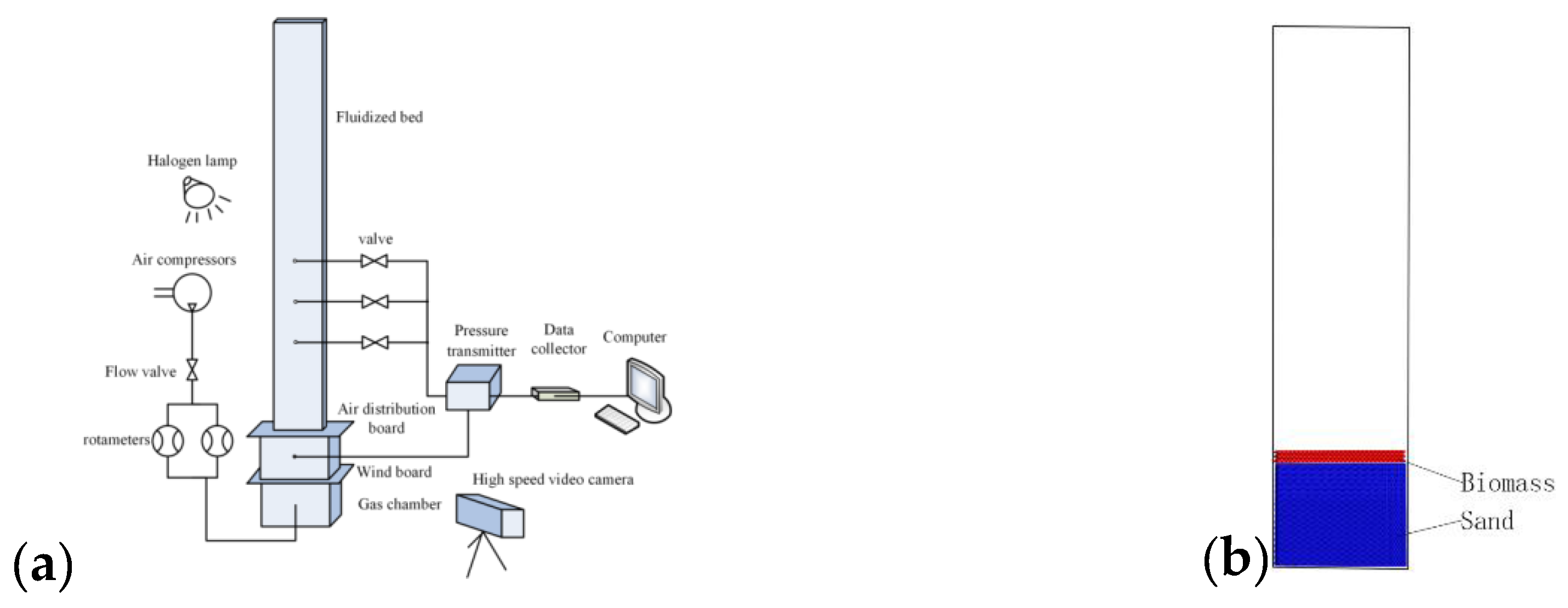
3. Experiment and Simulation Conditions

3.1. Experiment Details

Experiments are conducted on a lab-scale fluidized bed (30 mm × 120 mm × 1000 mm) to certify the simulation results. The schematic drawing of fluidized bed system is shown in Figure 1a [31]. Sands are packed on the bottom of bed and millet particles are arranged loose over sand. The condition of gas velocity set as 1 m/s, 1.5 m/s, and 2.5 m/s. Pressure drop is recorded by a pressure transmitter and data collecting system. Images are saved by high speed video. The height of sands is about 40 mm in all experiment initial arrangements. The experiments will provide pressure fluctuation and instantaneous images as a contrast validation for the simulation.

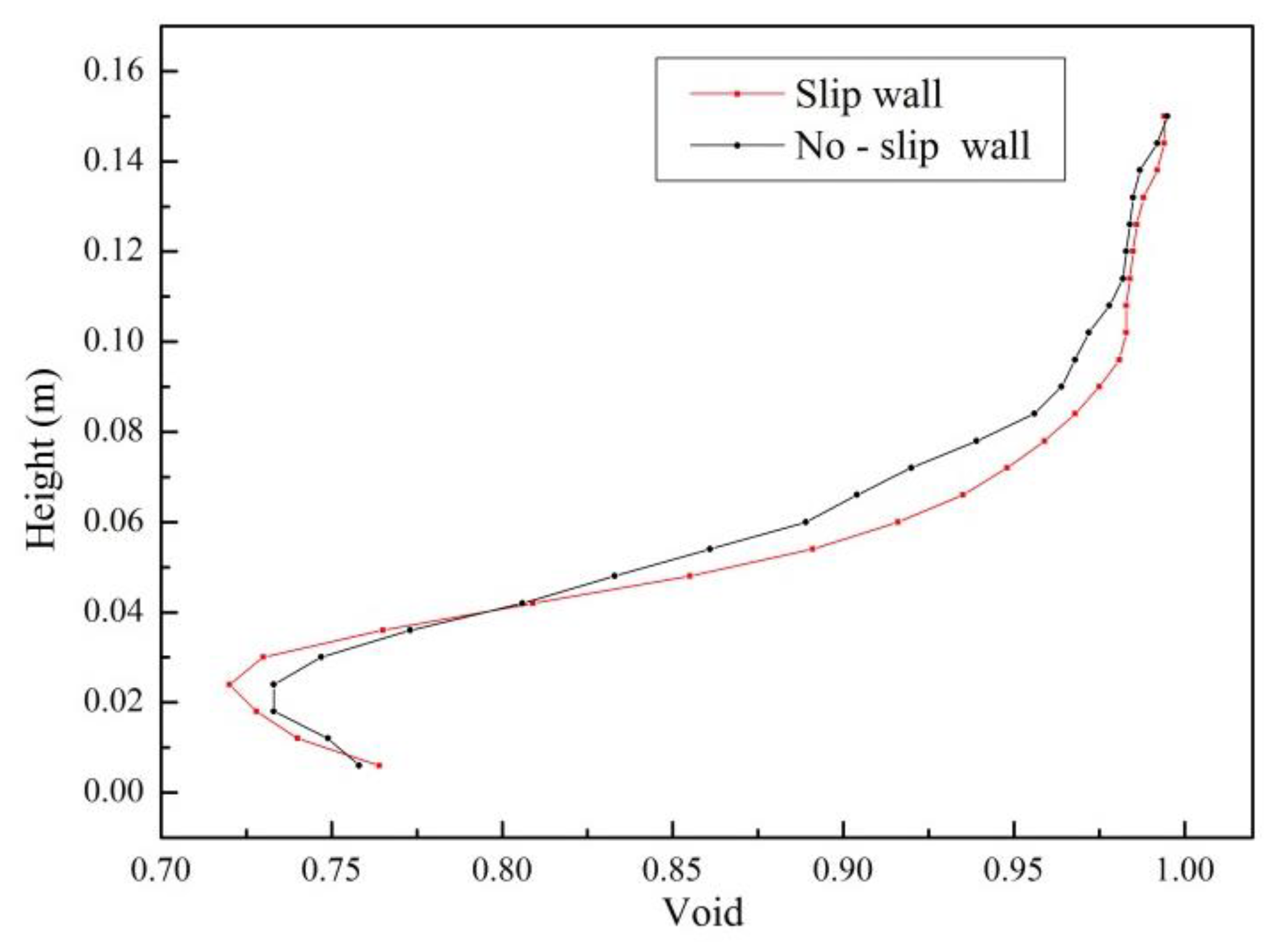
3.2. Simulation Conditions

Modeling is calculated by the in-lab code Multi-Flow [40]. In CFD frame, the calculation domain has same width and length as the experimental fluidized bed (30 mm × 120 mm) but considering the computational efficiency, the height of numerical model is 600 mm. The upside outlet boundary is a pressure-outlet. The setting of particles and bed features are listed in

Table 2. Simulation Details.

Parameters	Unit	Value
Diameter of sand	mm	0.8
Diameter of biomass particle	mm	1.5, 2, 3
Density of sand	kg/m3	2650
Density of biomass	kg/m3	1300
Density of gas	kg/m3	1.28
Velocity of gas	m/s	1.0 m/s, 1.5 m/s, 2.5 m/s
Viscosity of gas	Pa∙s	1.75 × 10−5
Wall young’s modulus	MPa	1 × 106
Wall friction coefficient		0.35
Wall restitution coefficient		0.9
Biomass Young’s modulus	Mpa	1.6 × 103
Biomass Possion ratio		0.4
Biomass friction coefficient		0.34
Biomass restitution coefficient		0.59
Biomass mass fraction		2%, 4%, 6%
Sand Young’s modulus	Mpa	1 × 106
Sand Possion ratio		0.33
Sand friction coefficient		0.35
Sand restitution coefficient		0.9
CFD Mesh size	mm	6 × 6 × 6
vmf	m/s	0.36, 0.4, 0.54

. Biomass particle properties such as Poisson’s ratio, Young’s modulus, friction coefficient and coefficient of restitution are referenced from reference [41]. The minimum fluidization velocity of mixing particles is estimated according to the empirical formula from reference [9].

Considering the calculation cost, the initial arrangement of the particles is different from the natural dense packed initialization in experiments. The initial particle position is shown in Figure 1b. Sands (blue) are arranged on the bottom of the fluidized bed and biomass particles (red) on the upside of sands. The number of particles would be the same as that in experiments but the space between particles is given as a quarter of the particle diameter. Because of the loose arrangement, the initial bed height would be much higher than that in experiments. Particle calculation tasks would assign to more processors due to the increasing number of mesh containing particles. Moreover, another reason to have a different initial arrangement is that the cost of calculation can sharply reduce as fewer particles need to be visit when calculate the contact force of particles. Sand particle number is 143120 in all cases. However, the quantity of biomass particles in each case is different when mass ratio is different as shown in

Table 3. Biomass number in each case.

Biomass Diameter	Mass Ratio
	2%	4%	6%
1.5 mm	903	1806	2708
2 mm	381	762	1143
3 mm	113	226	339

. The biomass particle number also varies when biomass size is different as the biomass ratio stays the same.

Searching distance is provided to find the nearby particles so the given space between particles would be sensitive to particle searching time. In present work, the searching distance is 1.05 times the host particle so a space of quarter diameter is enough to keep the calculation highly efficient in the initial calculation. The CFD time step is 10 × 10⁻⁶ s and the DEM time step is 10 × 10⁻⁷ s in the calculation. 20 processors are assigned for each case to conduct parallel calculations on a high performance computer. The actual calculation time of each case is around 4 weeks.

Particles mixture is complicated phenomenon and the mixing characteristics are influenced by many factors such as the bed size, biomass density, size, shape, mass fraction and gas velocity [42]. Moreover, each factor could interact on the mixing quality in fluidization [43]. In the present study, gas velocity, biomass density and biomass size are considered. Inlet gas velocity is the basis of fluidization so we investigate the mixing behavior in different gas velocities. Besides, Biomass particle size is an important parameter of mixing behavior so different biomass particle sizes are investigated. The wall slip condition is considered in our 3-D model, a test has been conducted before all simulation and a comparison of a near wall void fraction about the no – slip and slip wall condition is shown in Figure 2. The void fraction in near wall area is calculated by the time averaged. Void fraction has similar trend from bed bottom to the surface of bed height. The minimum and maximum void fraction appears at same height for both slip wall and no – slip wall condition. Gas velocity in the near wall area also have same trend as shown in Figure 3. A slight difference could be found, so a no slip wall condition is applied in all cases.

4. Results and Discussion

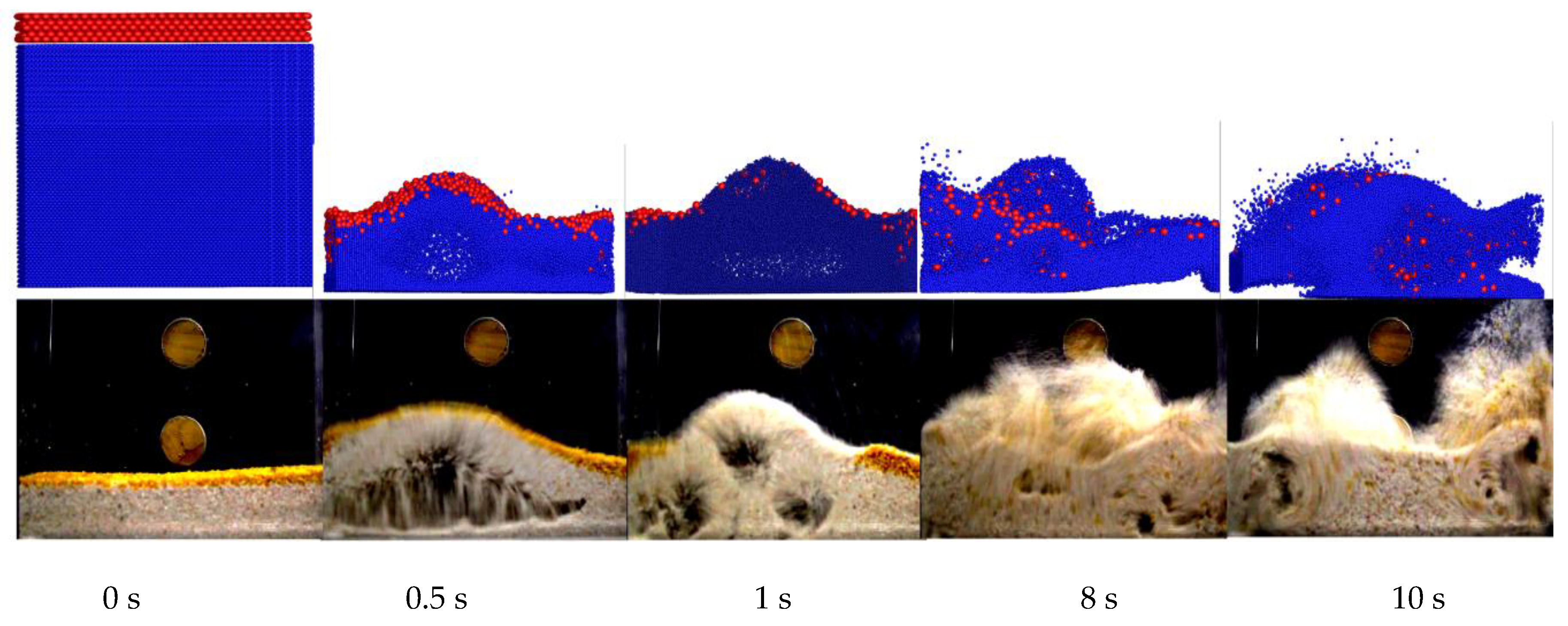
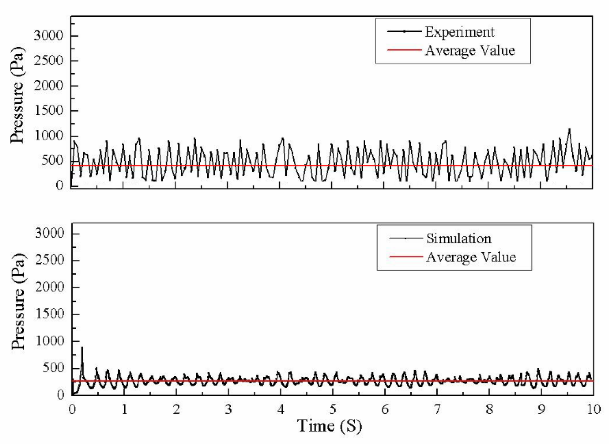
4.1. Validity of Simulation Results

Figure 4 is the snapshots of an instantaneous fluidized process from 0 s to 10 s of simulation and experiments. It can be seen that the fluidized processes agree well between the simulation and experiments. The bed height of simulation is higher than that of experiment at 0 s because of the loose arrangement. Then, the particles movement of both the simulation and the experiment are in accordance. Bubbles generate and rise up in the central area; particles are carried and pushed aside by bubbles.

The instantaneous pressure drop of the cases is shown in Figure 5. Pressure fluctuation period of the experiment is normally between 180 ms and 250 ms and the pressure fluctuation period of simulation is from 166 ms to 250 ms, which is basically in accordance. The value of averaged pressure drop in experiments and simulation is 412 Pa and 266 Pa. The different gas distribution may be the main reason for a larger pressure drop in the experiment. The time averaged value of empty bed pressure drop is measured as 155 Pa at the same condition, which due to the distribution plate and the wall effect. Considering the additional pressure loss in experiments, the simulation results are well matched with the experiment results. Pressure drop at the initial time could be affected by the particle arrangement as described in Section 3. Considering the mentioned hypothesis in simulation such as particle arrangement, mesh size and gas distribution, the simulation results are reasonable and valid.

4.2. Particle Mixing Characteristics at Different Gas Velocities

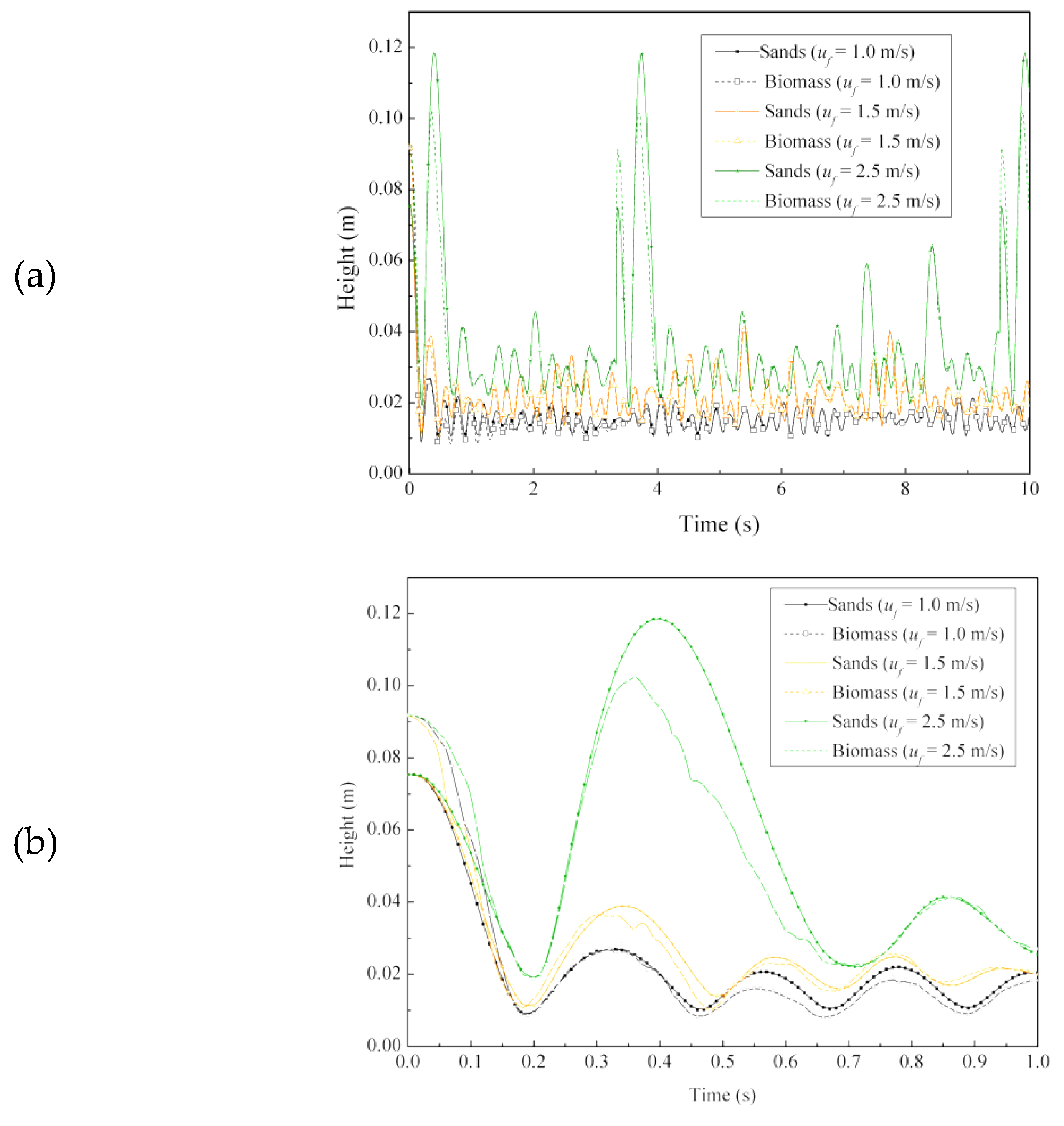
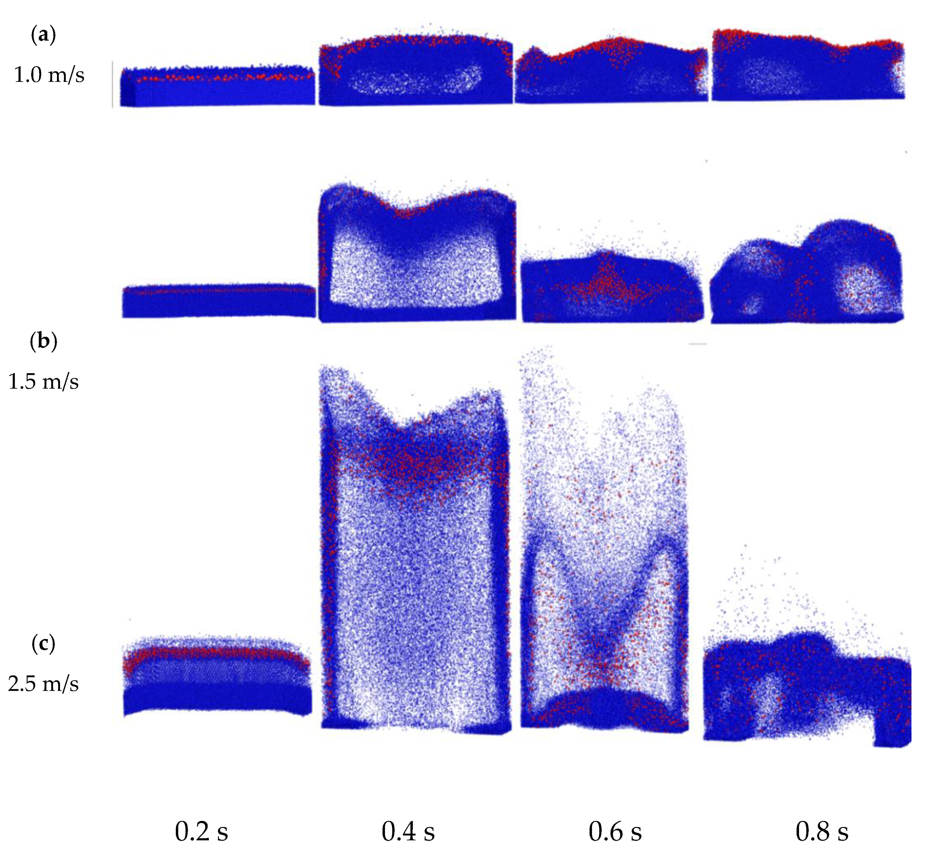
4.2.1. Instantaneous Particle Height

Instantaneous particle height is a critical factor of particle fluidization which can indirectly reflect the bubble and particles movement characteristics. The instantaneous height of biomass and sand particles are calculated separately as:

$$H_b={\displaystyle \sum _i^N{H}_i}/N_{biomass}$$

(15)

$$H_s={\displaystyle \sum _i^N{H}_i}/N_{sand}$$

(16)

in which, N_biomass is the number of biomass and N_sand is the number of sand.

The instantaneous height of biomass particles and sands at different gas velocities in 10 s is shown in Figure 6. The different colours, black, yellow and green, represent different gas velocities, 1.0 m/s, 1.5 m/s and 2.5 m/s. Both biomass and sand particles reach higher positions when the superficial velocity is higher. The fluctuation tends to be severe with the increasing of gas velocities. In each case, the instantaneous height of biomass particles and sands is similar in a late period but the difference in the initial period should be discussed. The details of particles time averaged height in the first second is shown in Figure 6b. Particle movement details would be better understood with an instantaneous snapshot. Particle instantaneous movements of the first second are shown in Figure 7. Particles in cases with 2.5 m/s arrived at the summit at 0.4 s, shown by the green line in Figure 6b. The cases with 1.0 m/s and 1.5 m/s have similar periods in Figure 7 but it could be observed that the particle movement period would be longer as the gas velocity increases and particles in the case with higher velocity would have higher bed height and mix better. It is clear that the different flow patterns of different velocities occur at the initial period in Figure 7. The red particles are still gathered in the top area at 0.8 s as shown in Figure 7a but as the gas velocity increases, particles become better mixed as shown in Figure 7b,c.

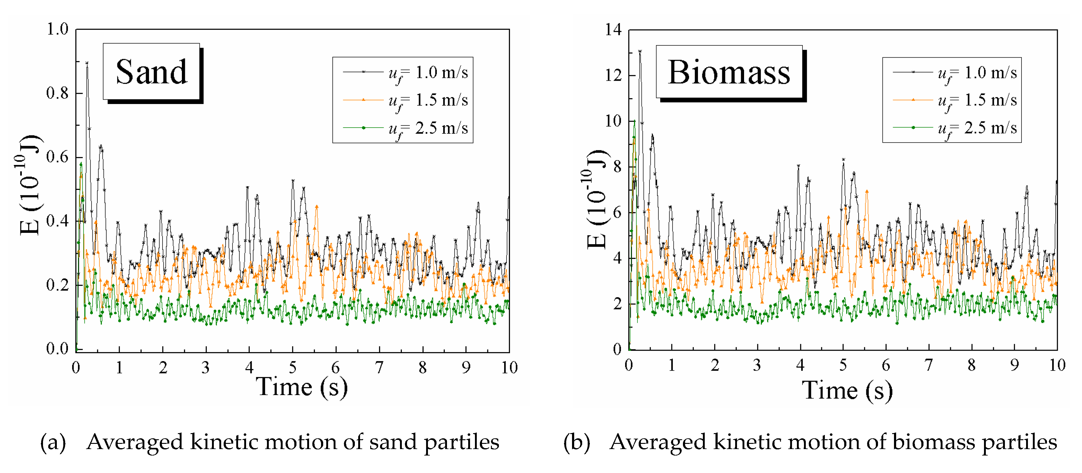
4.2.2. Particle Averaged Kinetic Energy

The difference movements between biomass and sand particles are generally discussed in Section 4.2.1. To explore individual particle motion, the particle averaged kinetic translational motion of biomass and sand are calculated separately and shown in Figure 8a,b. Both biomass and sand particles will get larger kinetic translational motion when the gas velocity is higher. Due to the fact that biomass density is half of sand density and the diameter of biomass is 2.5 times of sand diameter, the averaged kinetic translational motion of biomass is nearly 10 times that of sand particle motion in each case. Because of the large mass difference, the instantaneous height of sand can be higher than biomass. Consistent with Figure 8, the particle averaged kinetic translational motion of both biomass and sand has similar variation trend. The averaged kinetic translational motion reaches the highest value in the early period and fluctuates in a certain range based on different gas velocities.

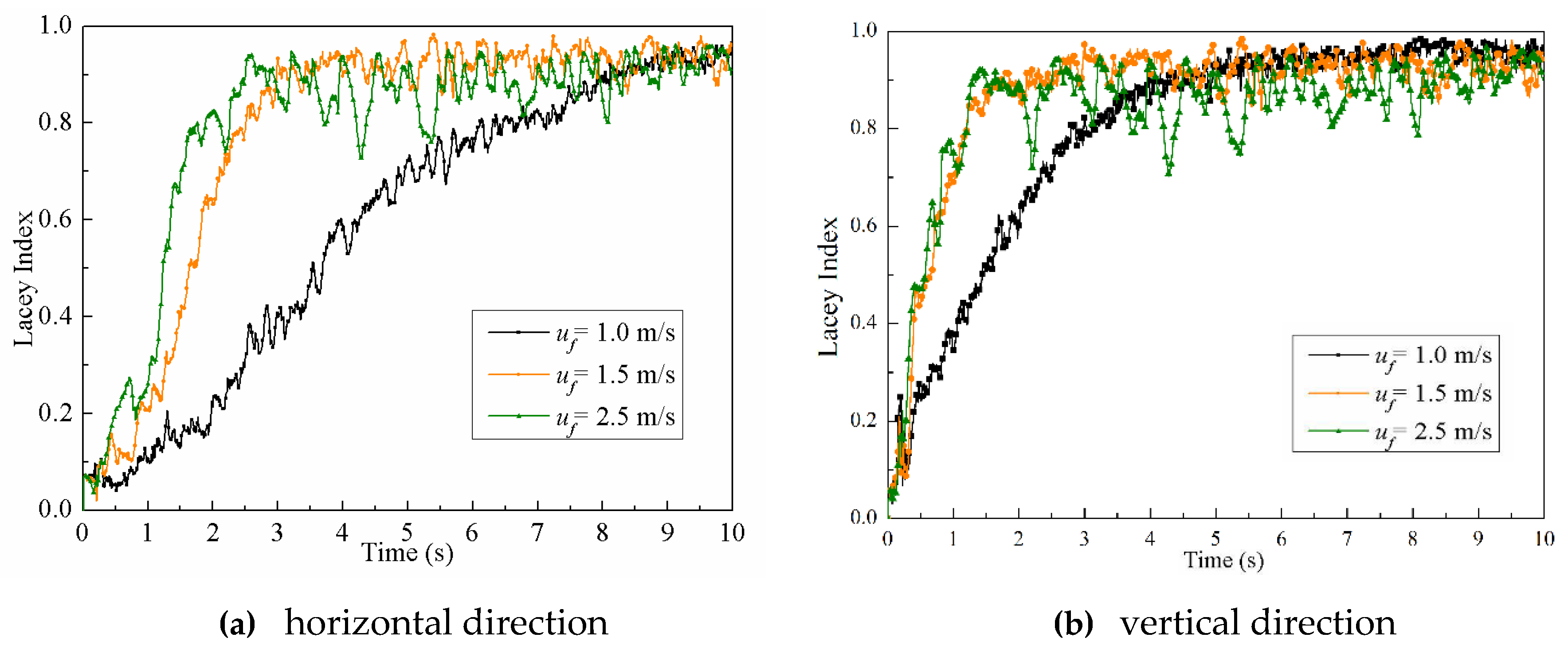
4.2.3. Particle Mixing Index

The Lacey index of biomass particles is shown in Figure 9. The Particles mixing index in both the vertical direction and horizontal direction are calculated. Particles are well mixed after 8 s in all three cases. Particles reach a well mixed state faster when the gas velocity is higher because of the more extensive gas solid interaction. However, the mixing state is not stable when the gas velocity is too high. Particles may separate because of the intensive gas movement, which can involve a sudden rupture of large bubbles. It is clear to see that there were two sharp drops between 4 and 6 s when the gas velocity is 2.5 m/s as the line in green shows in Figure 9a,b. Particles in low velocity mix more slowly in a horizontal direction because particles get less motion with low gas velocity. Particles mix faster and better in a vertical direction than in a horizontal direction in all three cases. In this regard, the case is in the best mixing condition of the three simulation cases when the gas velocity is 1.5 m/s.

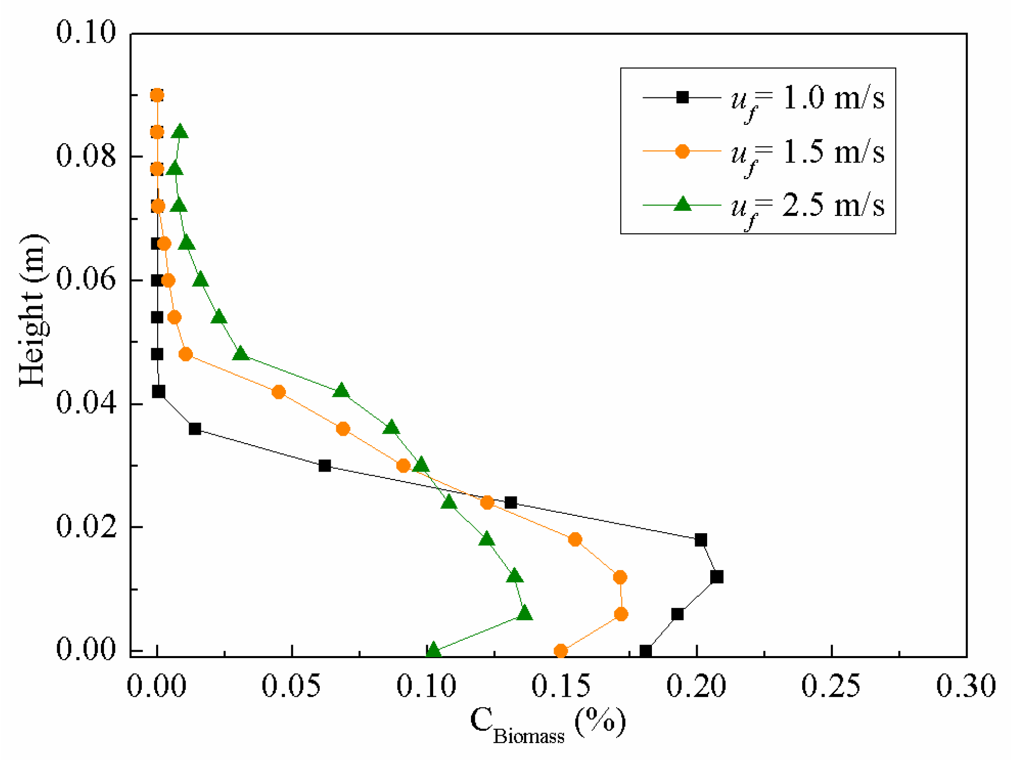
4.2.4. Time Averaged Biomass Distribution

After the study of instantaneous information, it is necessary to discuss the mixing state after reaching a well mixed state. In particular, the relation of gas velocity and the biomass particle distribution by height should be studied. The time-averaged biomass particle distribution is the ratio of the weight of biomass at a certain height to the total biomass weight as shown in Figure 10. Comparing the cases with different velocities, it could be observed that from bottom to top, the biomass time-averaged concentration in each case have a similar trend by growing firstly and then dropping to nearly zero. Combined with the discussion of the former section, particles would have a larger kinetic motion when gas velocity is larger, so the case of higher gas velocities have more particles in the higher area and less in the lower area.

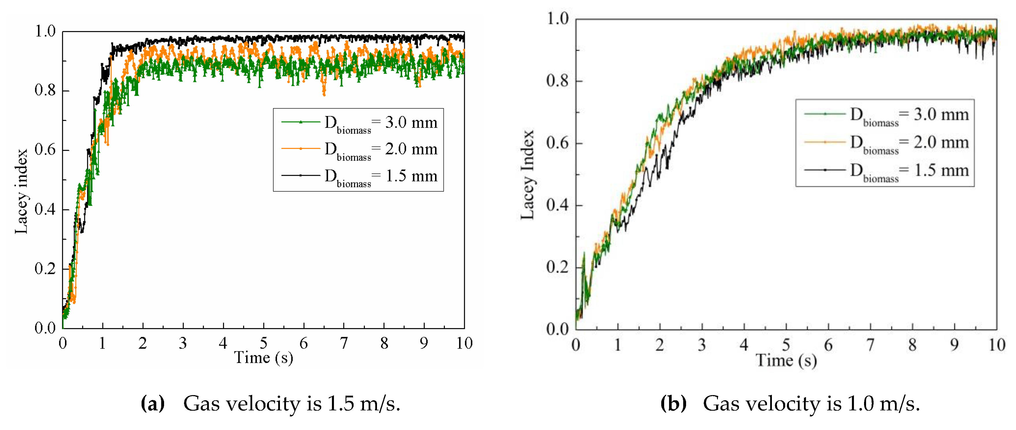
4.3. Particle Mixing Characteristics with Different Biomass Particle Sizes

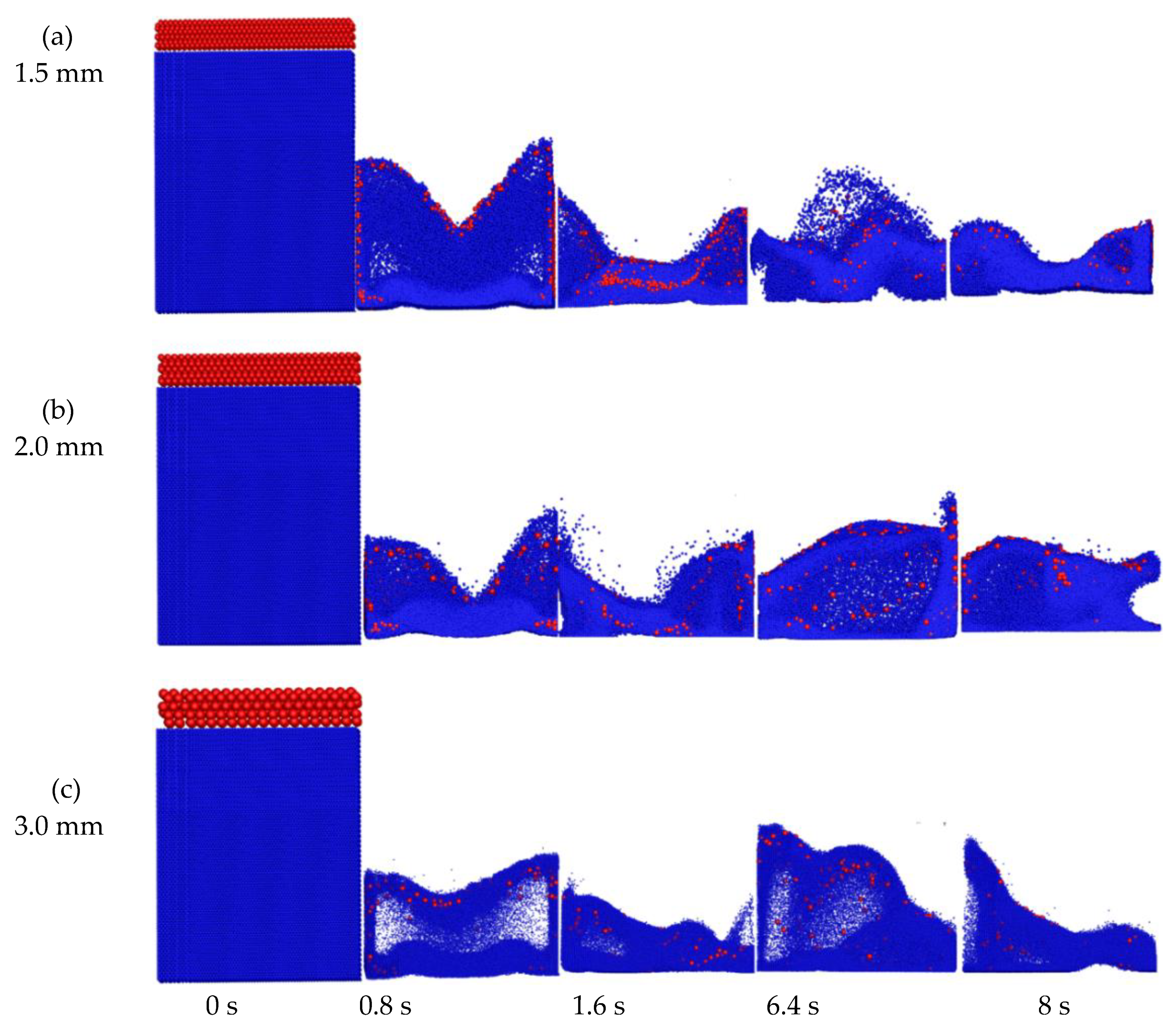
4.3.1. Instantaneous Particle Mixing Behavior

Biomass particle size is one of the critical parameters because the large sized difference between biomass particles and sand is very common in industry utilization.

The distribution of biomass and sand particles in each cell are investigated to provide more mixing details at the local position. To ensure the simulation results in a well fluidized condition, the gas velocity of all cases in this section is 1.5 m/s according to the discussion of the former section. Particle instantaneous snapshots are shown in Figure 11. The mixing processes of biomass and sands in all three cases have a similar trend. Biomass particles fell around near wall area firstly (0.8 s) and then sands rose and mixed with biomass. Particles are well mixed after around 8 s. The instantaneous distribution and movements of biomass particles in all three mixing processes are different as the size changed.

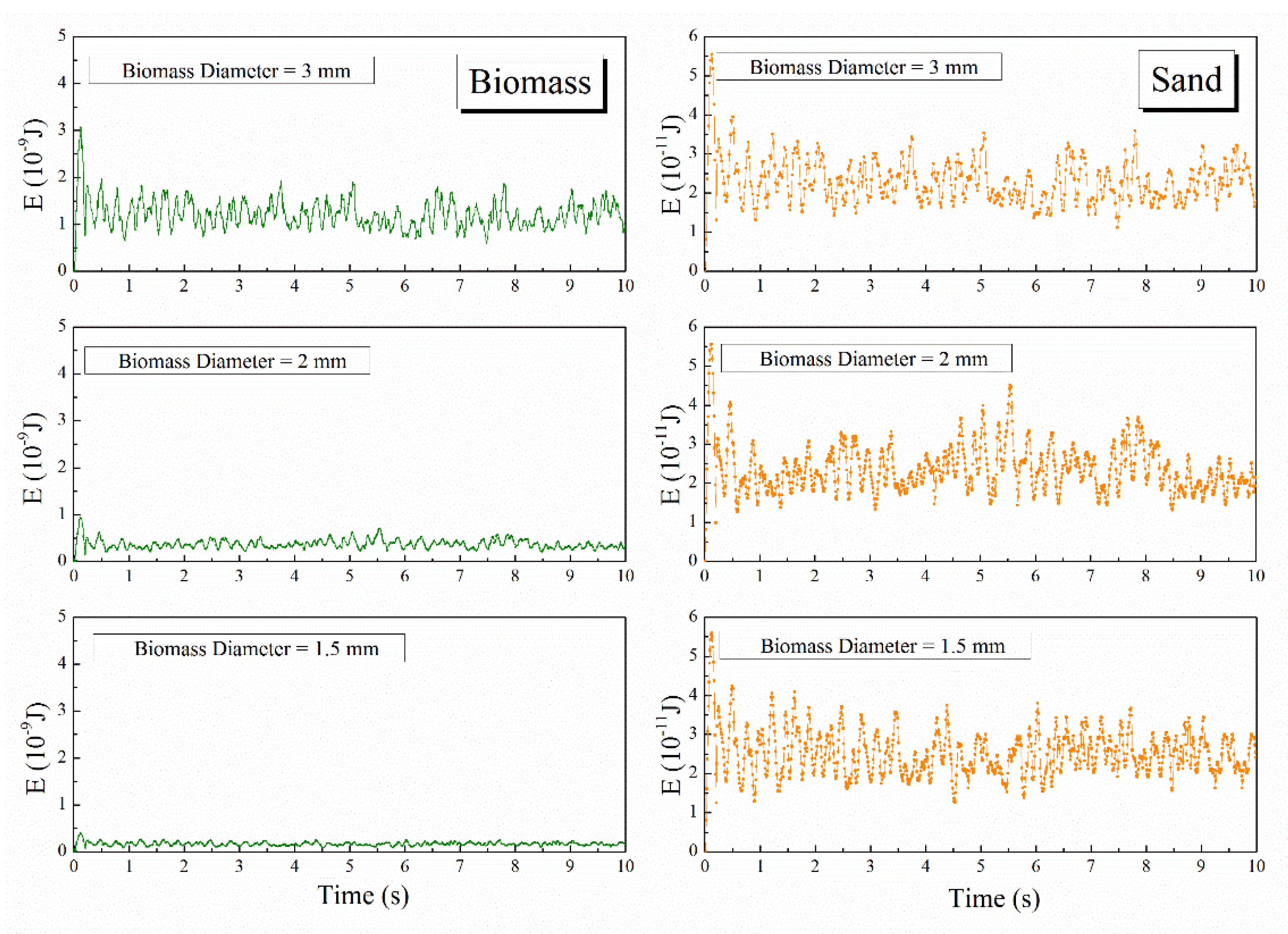
4.3.2. Particle Averaged Kinetic Energy

To explore the size effect on individual particle motion, the particle averaged kinetic translational motion of biomass and sand are calculated separately and shown in Figure 12. Sands motion has similar value in all three cases but biomass motion has a sharp increase when the size becomes large. The integrate fluctuation also becomes strong when biomass particles is large. The motion of biomass particle is larger than sand. Even for the smallest biomass, single biomass still has 10 times the motion of sand.

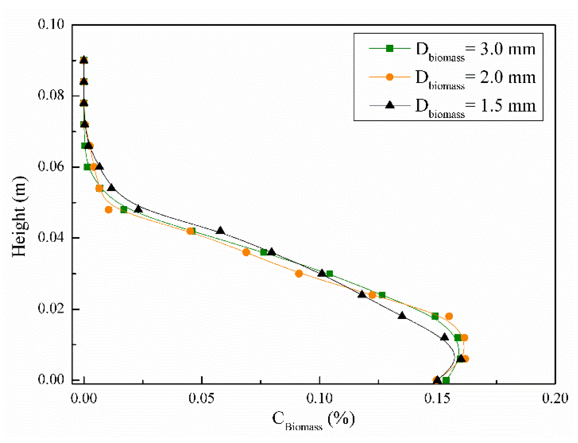
4.3.3. Time Averaged Biomass Distribution

It is helpful to understand the dynamic mixing process of biomass particles and sands from Figure 9. However, it is not the objective to get a clear relationship between the biomass particle size and mixing trend only according to the instantaneous position. Time-averaged concentration of biomass particles by height is shown in Figure 13. The data is extracted between 8 s and 10 s when the fluidized state is fully stable. The overall variation trend of all three cases is extremely similar as discussed in the last section but the changing of biomass size barely affects the results. Probably, in a well mixed condition, size difference in the range of 2 to 4 times may not affect the biomass distribution in a vertical direction. However, due to being limited by the mesh size and the ratio of mesh size and particle size, it is not suitable to conduct a larger size difference in present calculation model.

The Lacey mixing index of the case with different biomass particle diameters in vertical direction is shown in Figure 14. Comparing the results of all three cases, smaller size difference of biomass particles and sands could lead to a better mixing state and also reach the stable mixing state faster. However, even with the largest size difference as the green line shown in Figure 14, the case could keep a high Lacey index over 0.8 when gas velocity is 1.5 m/s. Figure 14b has a particle mixing quality at 1.0 m/s gas velocity. The Lacey index of the case with large biomass particles has a slightly quicker rise than that with 1 mm diameter biomass particles. Comparing the Lacey index of Figure 9 and Figure 14, the biomass particles size is not as sensitive as gas velocity to the mixing behavior.

5. Conclusions

The Biomass particle and sands mixing process is complicated but significant for biomass chemical utilization. The simulation method could provide the details of particle movement and mixing process. Our study has built a model of a biomass particle and sands mixing process in a Euler – Lagrange frame. The large size and density difference between biomass particles and sands leads to complicated fluidizing and mixing behavior. This present study has focused on the effectiveness of particle size, gas velocity. Particle instantaneous averaged height, particle distribution, particle motion and Lacey index of each case are discussed. Some conclusions could be drawn based on the analyzing of simulation results: Increasing gas velocity in a reasonable range can accelerate the mixing process but can also enhance the fluctuation. Compared to biomass particle size, gas velocity is more sensitive to the mixing quality. Size difference could slightly affect the mixing quality on the condition that the gas velocity is suitable and it is found that a smaller size difference would lead to a better mixing process. In the view of the present study, biomass particles and sands could be well mixed if the size difference is smaller than 4 times.

References

1. Sher, F.; Pans, M.A.; Afilaka, D.T.; Sun, C.; Liu, H. Experimental investigation of woody and non-woody biomass combustion in a bubbling fluidised bed combustor focusing on gaseous emissions and temperature profiles. Energy 2017, 141, 2069–2080. [Google Scholar] [CrossRef]
2. Sher, F.; Pans, M.A.; Sun, C.; Snape, C.; Liu, H. Oxy-fuel combustion study of biomass fuels in a 20 kW(th) fluidized bed combustor. Fuel 2018, 215, 778–786. [Google Scholar] [CrossRef]
3. Ku, X.; Li, T.; Lovas, T. CFD-DEM simulation of biomass gasification with steam in a fluidized bed reactor. Chem. Eng. Sci. 2015, 122, 270–283. [Google Scholar] [CrossRef]
4. Zhang, Y.; Jin, B.S.; Zhong, W.Q.; Ren, B.; Xiao, R. Characterization of Fluidization and Segregation of Biomass Particles by Combining Image Processing and Pressure Fluctuations Analysis. Int. J. Chem. React. Eng. 2009, 7. [Google Scholar] [CrossRef]
5. Sun, Q.Q.; Lu, H.L.; Liu, W.T.; He, Y.R.; Yang, L.D.; Gidaspow, D. Simulation and experiment of segregating/mixing of rice husk-sand mixture in a bubbling fluidized bed. Fuel 2005, 84, 1739–1748. [Google Scholar]
6. Madhlyanon, T.; Piriyarungroj, N.; Soponronnarit, S. Cold flow behavior study in novel cyclonic fluidized bed combustor (psi-FBC). Energy Convers. Manag. 2008, 49, 1202–1210. [Google Scholar] [CrossRef]
7. Formisani, B.; Girimonte, R.; Vivacqua, V. Fluidization of Mixtures of Two Solids Differing in Density or Size. AIChE J. 2011, 57, 2325–2333. [Google Scholar] [CrossRef]
8. Leon, M.A.; Dutta, A. Fluidization Characteristics of Rice Husk in A Bubbling Fluidized Bed. Can. J. Chem. Eng. 2010, 88, 18–22. [Google Scholar] [CrossRef]
9. Zhong, W.Q.; Jin, B.S.; Zhang, Y.; Wang, X.F.; Xiao, R. Fluidization of Biomass Particles in a Gas-Solid Fluidized Bed. Energy Fuel 2008, 22, 4170–4176. [Google Scholar] [CrossRef]
10. Si, C.D.; Guo, Q.J. Fluidization Characteristics of Binary Mixtures of Biomass and Quartz Sand in an Acoustic Fluidized Bed. Ind. Eng. Chem. Res. 2008, 47, 9773–9782. [Google Scholar] [CrossRef]
11. Rao, K.; Reddy, G.V. Cold Flow Studies of Rice Husk, Saw Dust, and Groundnut Shell Fuels in a Fluidized Bed. Energy Sources Part A—Recovery Util. Environ. Eff. 2010, 32, 1701–1711. [Google Scholar] [CrossRef]
12. Palappan, K.G.; Sai, P.S.T. Studies on segregation of binary mixture of solids in continuous fast fluidized bed. Chem. Eng. J. 2008, 139, 330–338. [Google Scholar] [CrossRef]
13. Zhong, W.Q.; Xiong, Y.Q.; Yuan, Z.L.; Zhang, M.Y. DEM simulation of gas-solid flow behaviors in spout-fluid bed. Chem. Eng. Sci. 2006, 61, 1571–1584. [Google Scholar] [CrossRef]
14. Zhao, X.J.; Eri, Q.T.; Wang, Q. An Investigation of the Restitution Coefficient Impact on Simulating Sand-Char Mixing in a Bubbling Fluidized Bed. Energies 2017, 10, 617. [Google Scholar] [CrossRef]
15. Zhuang, Y.Q.; Chen, X.M.; Luo, Z.H.; Xiao, J. CFD-DEM modeling of gas-solid flow and catalytic MTO reaction in a fluidized bed reactor. Comput. Chem. Eng. 2014, 60, 1–16. [Google Scholar] [CrossRef]
16. Amiri, Z.; Movahedirad, S. Bubble-induced particle mixing in a 2-D gas-solid fluidized bed with different bed aspect ratios: A CFD-DPM study. Powder Technol. 2017, 320 (Suppl. C), 637–645. [Google Scholar] [CrossRef]
17. Saidi, M.; Tabrizi, H.B.; Grace, J.R.; Lim, C.J.; Ahmad, G. Hydrodynamic and Mixing Characteristics of Gas-Solid Flow in a Pulsed Spouted Bed. Ind. Eng. Chem. Res. 2015, 54, 7933–7941. [Google Scholar] [CrossRef]
18. Xu, H.B.; Zhong, W.Q.; Yuan, Z.L.; Yu, A.B. CFD-DEM study on cohesive particles in a spouted bed. Powder Technol. 2017, 314, 377–386. [Google Scholar] [CrossRef]
19. Xu, Y.; Musser, J.; Li, T.; Gopalan, B.; Panday, R.; Tucker, J.; Breault, G.; Clarke, M.A.; Rogers, W.A. Numerical Simulation and Experimental Study of the Gas-Solid Flow Behavior Inside a Full-Loop Circulating Fluidized Bed: Evaluation of Different Drag Models. Ind. Eng. Chem. Res. 2018, 57, 740–750. [Google Scholar] [CrossRef]
20. Wang, J. A Review of Eulerian Simulation of Geldart a Particles in Gas-Fluidized Beds. Ind. Eng. Chem. Res. 2009, 48, 5567–5577. [Google Scholar] [CrossRef]
21. Oke, O.; Van Wachem, B.; Mazzei, L. Lateral solid mixing in gas-fluidized beds: CFD and DEM studies. Chem. Eng. Res. Des. 2016, 114 (Suppl. C), 148–161. [Google Scholar] [CrossRef]
22. Liu, D.; Chen, X. Quantifying lateral solids mixing in a fluidized bed by modeling the thermal tracing method. AIChE J. 2012, 58, 745–755. [Google Scholar] [CrossRef]
23. Pantaleev, S.; Yordanova, S.; Janda, A.; Marigo, M.; Ooi, J.Y. An experimentally validated DEM study of powder mixing in a paddle blade mixer. Powder Technol. 2017, 311, 287–302. [Google Scholar] [CrossRef]
24. Luo, K.; Wu, F.; Yang, S.L.; Fan, J.R. CFD-DEM study of mixing and dispersion behaviors of solid phase in a bubbling fluidized bed. Powder Technol. 2015, 274, 482–493. [Google Scholar] [CrossRef]
25. Ma, H.Q.; Zhao, Y.Z. CFD-DEM investigation of the fluidization of binary mixtures containing rod-like particles and spherical particles in a fluidized bed. Powder Technol. 2018, 336, 533–545. [Google Scholar] [CrossRef]
26. Feng, Y.Q.; Xu, B.H.; Zhang, S.J.; Yu, A.B.; Zulli, P. Discrete particle simulation of gas fluidization of particle mixtures. AIChE J. 2004, 50, 1713–1728. [Google Scholar] [CrossRef]
27. Deb, S.; Tafti, D.K. Two and three dimensional modeling of fluidized bed with multiple jets in a DEM–CFD framework. Particuology 2014, 16, 19–28. [Google Scholar] [CrossRef]
28. Njobuenwu, D.O.; Fairweather, M. Dynamics of single, non-spherical ellipsoidal particles in a turbulent channel flow. Chem. Eng. Sci. 2015, 123, 265–282. [Google Scholar] [CrossRef]
29. Van Wachem, B.; Zastawny, M.; Zhao, F.; Mallouppas, G. Modelling of gas-solid turbulent channel flow with non-spherical particles with large Stokes numbers. Int. J. Multiph. Flow 2015, 68, 80–92. [Google Scholar] [CrossRef]
30. Wang, X.; Zhong, Z.; Wang, H.; Wang, Z. Application of Hilbert-Huang transformation in fluidized bed with two-component (biomass particles and quartz sands) mixing flow. Korean J. Chem. Eng. 2014, 32, 43–50. [Google Scholar] [CrossRef]
31. Zhu, L.L.; Zhong, Z.P.; Wang, H.; Wang, Z.Y. Simulation of large biomass pellets in fluidized bed by DEM-CFD. Korean J. Chem. Eng. 2016, 33, 3021–3028. [Google Scholar] [CrossRef]
32. Ergun, S. Fluid flow through oached columns. Chem. Eng. Prog. 1952, 48, 89–94. [Google Scholar]
33. Wen, C.Y.; Yu, Y.H. A Generalized Method for Predicting Minimum Fluidization Velocity. AIChE J. 1966, 12, 610–612. [Google Scholar] [CrossRef]
34. Rowe, P.N.; Henwood, G.A.; United Kingdom Atomic Energy Authority. Drag Forces in a Hydraulic Model of a Fluidised Bed—Part I; UKAEA: London, UK, 1960.
35. Cundall, P.A.; Strack, O.D.L. Discrete Numerical-Model for Granular Assemblies. Geotechnique 1979, 29, 47–65. [Google Scholar] [CrossRef]
36. Tsuji, Y.; Kawaguchi, T.; Tanaka, T. Discrete particle simulation of two-dimensional fluidized bed. Powder Technol. 1993, 77, 79–87. [Google Scholar] [CrossRef]
37. Bruchmüller, J.; van Wachem, B.; Gu, S.; Luo, K.; Brown, R. Modeling the thermochemical degradation of biomass inside a fast pyrolysis fluidized bed reactor. AIChE J. 2012, 58, 3030–3042. [Google Scholar] [CrossRef]
38. Lacey, P.M.C. Developments in The Theory of Particle Mixing. J. Appl. Chem. 1954, 4, 257–268. [Google Scholar] [CrossRef]
39. Wang, H.; Zhong, Z.; Wang, X.; Guo, F. Intelligent identification of the flow regimes of two-component particles in a fluidized bed with the optimized fuzzy c-means clustering algorithm. Korean J. Chem. Eng. 2016, 33, 1674–1680. [Google Scholar] [CrossRef]
40. Zhao, F.; George, W.K.; van Wachem, B.G.M. Four-way coupled simulations of small particles in turbulent channel flow: The effects of particle shape and Stokes number. Phys. Fluids 2015, 27, 083301. [Google Scholar] [CrossRef]
41. Chung, Y.C.; Ooi, J.Y. A study of influence of gravity on bulk behavior of particulate solid. Particuology 2008, 6, 467–474. [Google Scholar] [CrossRef]
42. Zhong, W.Q.; Zhang, Y.; Jin, B.S.; Zhang, M.Y. Discrete Element Method Simulation of Cylinder-Shaped Particle Flow in a Gas-Solid Fluidized Bed. Chem. Eng. Technol. 2009, 32, 386–391. [Google Scholar] [CrossRef]
43. Norouzi, H.R.; Mostoufi, N.; Mansourpour, Z.; Sotudeh-Gharebagh, R.; Chaouki, J. Characterization of solids mixing patterns in bubbling fluidized beds. Chem. Eng. Res. Des. 2011, 89, 817–826. [Google Scholar] [CrossRef]
Figure 1. (a) The experiment system [39]; (b) particles initial position in simulation.
Energies 12 01801 g001
Figure 2. Void fraction in the near wall area. (Simulation case: Biomass diameter is 2 mm; Sand diameter is 0.8 mm; gas velocity is 2.0 m/s.).
Energies 12 01801 g002
Figure 3. Gas velocity in the near wall area. (Simulation case: Biomass diameter is 2 mm; Sand diameter is 0.8 mm; gas velocity is 2.0 m/s.).
Energies 12 01801 g003
Figure 4. Snapshots of the instantaneous fluidized process. (Simulation case: Biomass diameter is 2 mm; Sand diameter is 0.8 mm; gas velocity is 1.0 m/s. Experiment case: Millet is the biomass particles used in experiments; gas velocity is 1.0 m/s. Biomass mass fraction is 6 % in both simulation and experiments.).
Energies 12 01801 g004
Figure 5. Pressure drop comparison of experiment and simulation. (Simulation case: Biomass diameter is 2 mm; Sand diameter is 0.8 mm; gas velocity is 1.0 m/s. Experiment case: Millet is the biomass particles used in experiments; gas velocity is 1.0 m/s. Biomass mass fraction is 6% in both simulation and experiments.).
Energies 12 01801 g005
Figure 6. The instantaneous average height of particles (Biomass diameter is 2 mm). (a) is a period of 10 s and (b) is the details of the first second.
Energies 12 01801 g006
Figure 7. Snapshots of particles instantaneous movements.
Energies 12 01801 g007
Figure 8. Averaged particle kinetic motion. (Biomass particle diameter is 2 mm.).
Energies 12 01801 g008
Figure 9. Lacey index Biomass (Biomass particle diameter is 2 mm.).
Energies 12 01801 g009
Figure 10. Time averaged biomass concentration by height. Time range is from 8 s to 10 s. Biomass particle diameter is 2 mm.
Energies 12 01801 g010
Figure 11. Snapshots of particles instantaneous movements. (a) biomass particle size is 1.5 mm; (b) biomass particle size is 2.0 mm; (c) biomass particle size is 3.0 mm; sand diameter is 0.8 mm and gas velocity is 1.5 m/s in all three cases).
Energies 12 01801 g011
Figure 12. Averaged particle kinetic motion. (Gas velocity is 1.5 m/s.).
Energies 12 01801 g012
Figure 13. Time averaged biomass concentration by height. (Gas velocity is 1.5 m/s.).
Energies 12 01801 g013
Figure 14. Lacey index.
Energies 12 01801 g014