A Time-Efficient and Accurate Open Circuit Voltage Estimation Method for Lithium-Ion Batteries

Abstract
:1. Introduction
2. Data Processing Algorithm
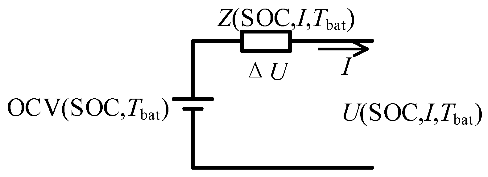
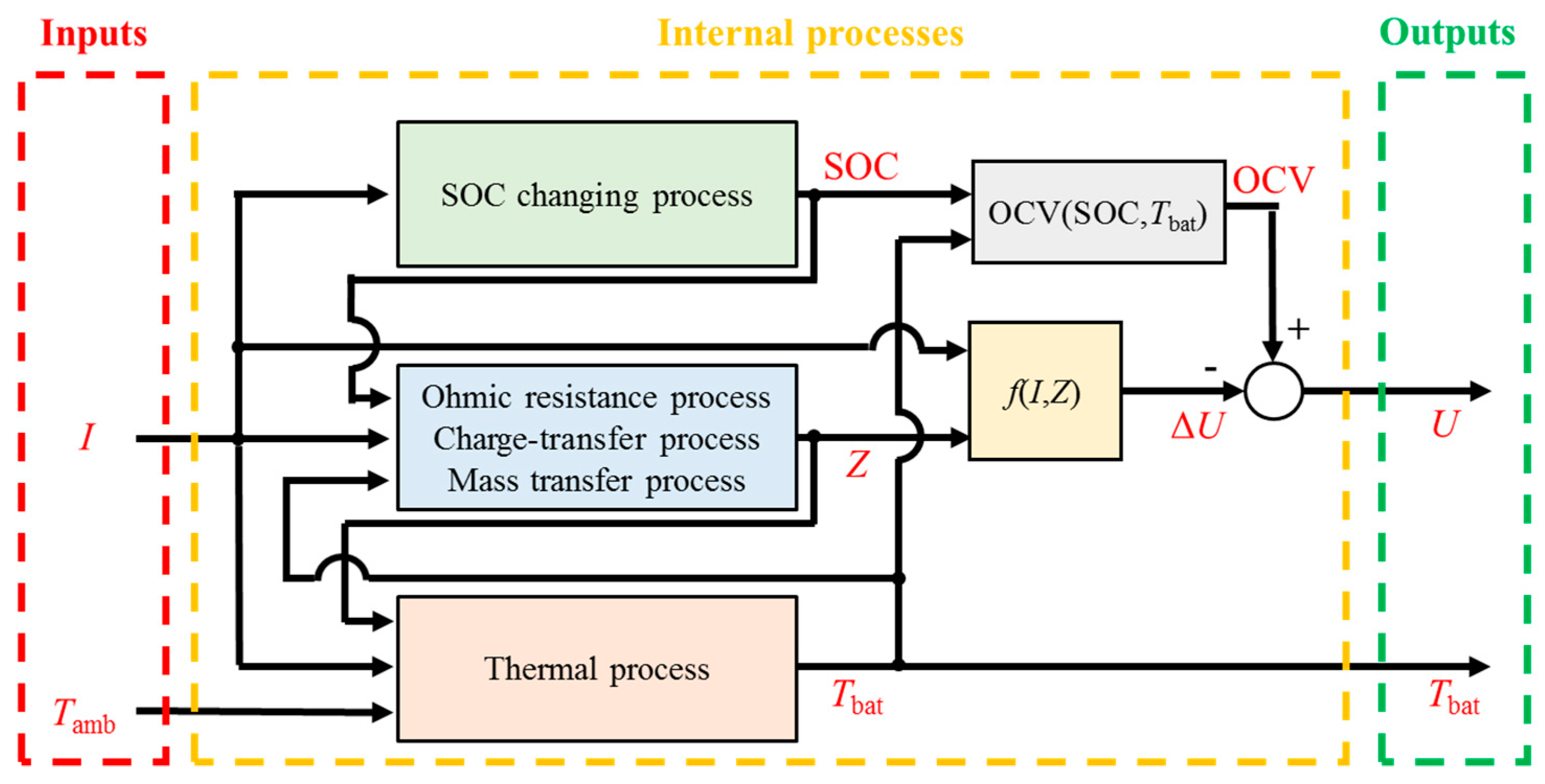
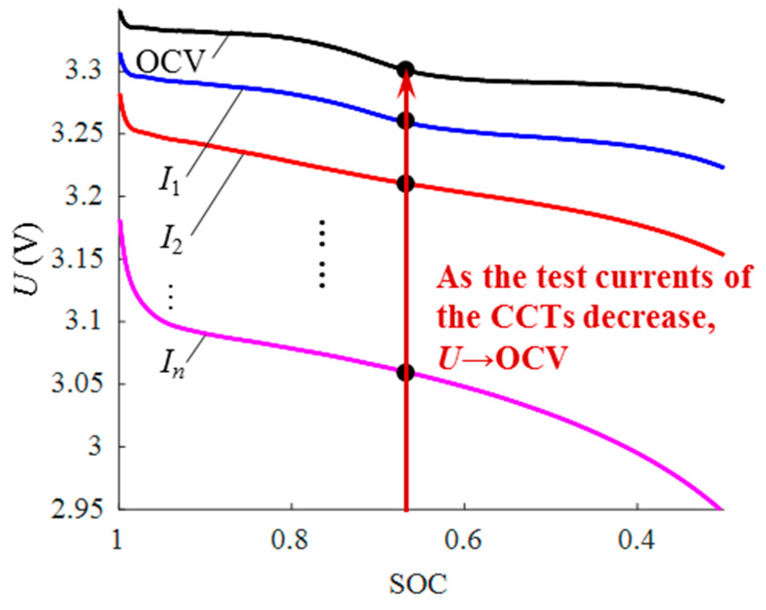
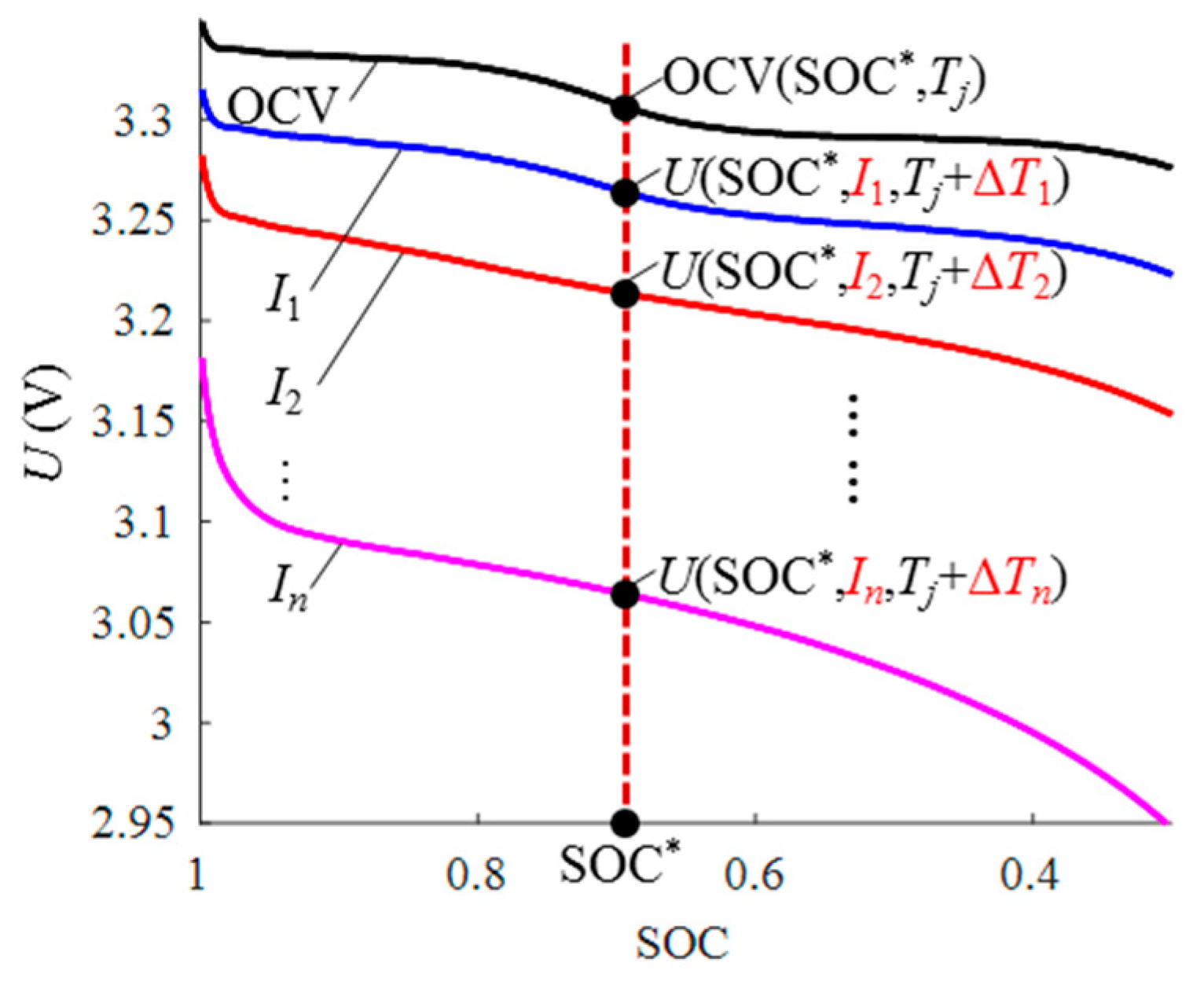
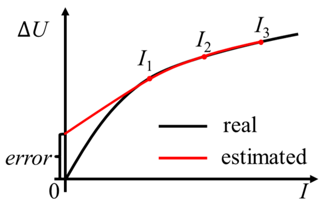
2.1. Algorithm Principle
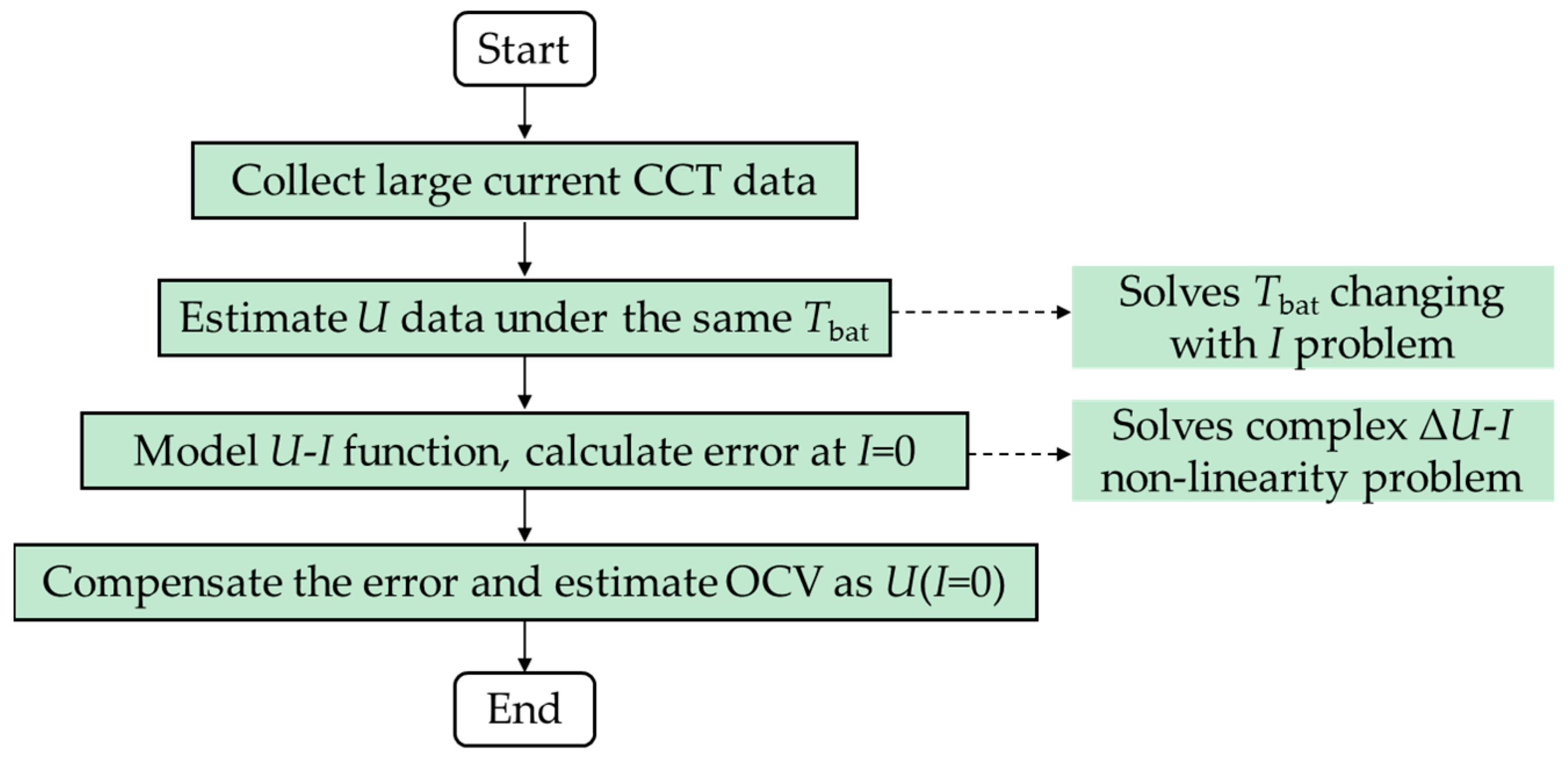
2.2. Algorithm Procedures
3. Experimental Design
3.1. Example of Experimental Procedures
3.1.1. Constant Current Test Procedures
- (1)
- Charge the battery using the standard procedures from the battery manufacturer. That is, charge the battery with I = −0.5 C, then start constant voltage charging when U = 3.6 V. Charging is completed when I = −0.02 C;
- (2)
- Immediately after charging is completed, change Tamb from 25 °C to Tj (Tj ∈ {5,15,25,35,45,55} °C and rest the battery for 2.5 h to make Tbat = Tj and the battery’s internal processes steady;
- (3)
- Discharge the battery with Ii (Ii ∈ {0.2,0.6,1.0,1.4,1.8,2.2} C). Discharging is completed when U = 2.5 V;
- (4)
- Immediately after discharge is completed, adjust Tamb to 25 °C and rest the battery for 0.5 h to let the internal processes approach steady. Then start the next CCT.
3.1.2. OCV True Value Measurement Test Procedures
3.2. Experimental Parameter Design
3.2.1. SOCref Design
SOCref Influence on Estimation Accuracy
SOCref Influence on Experimental Time
3.2.2. Design of Specific Value of {I1,I2,…,In} and Number n
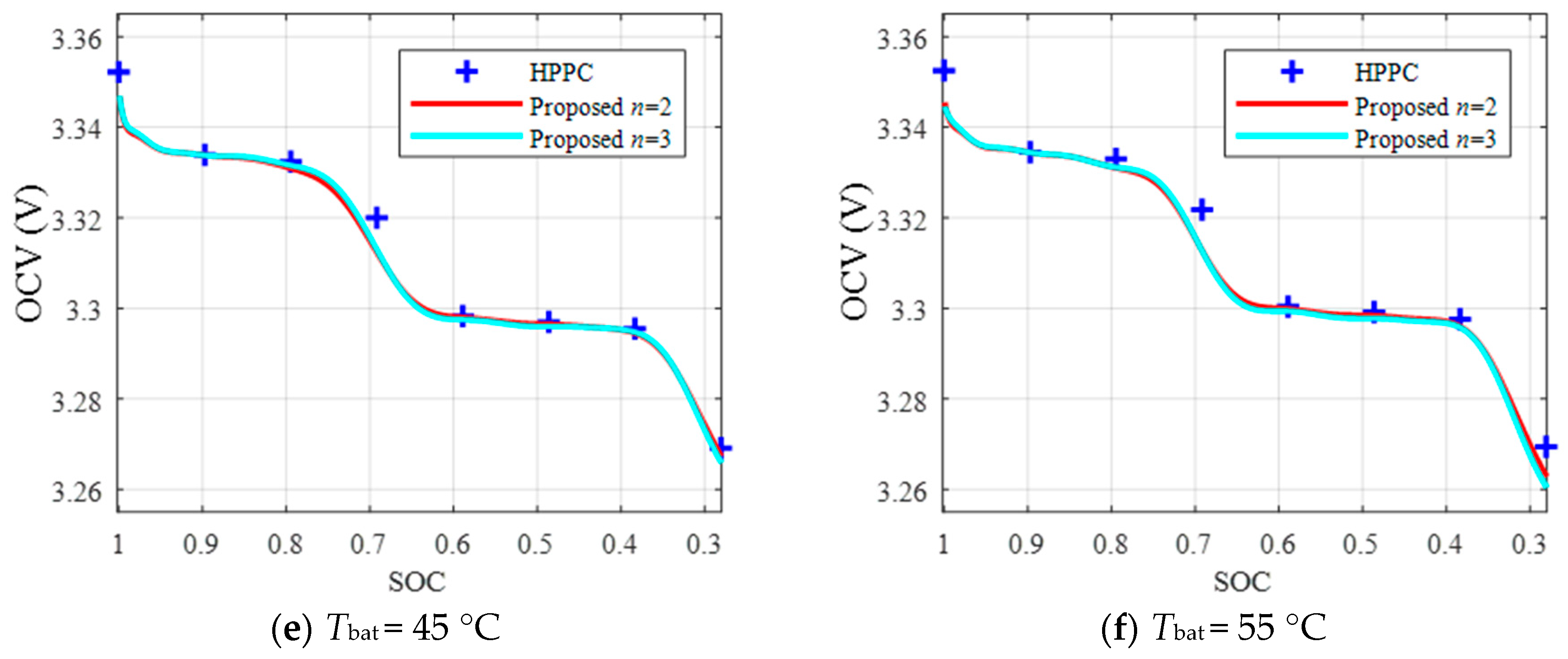
Design of Number n
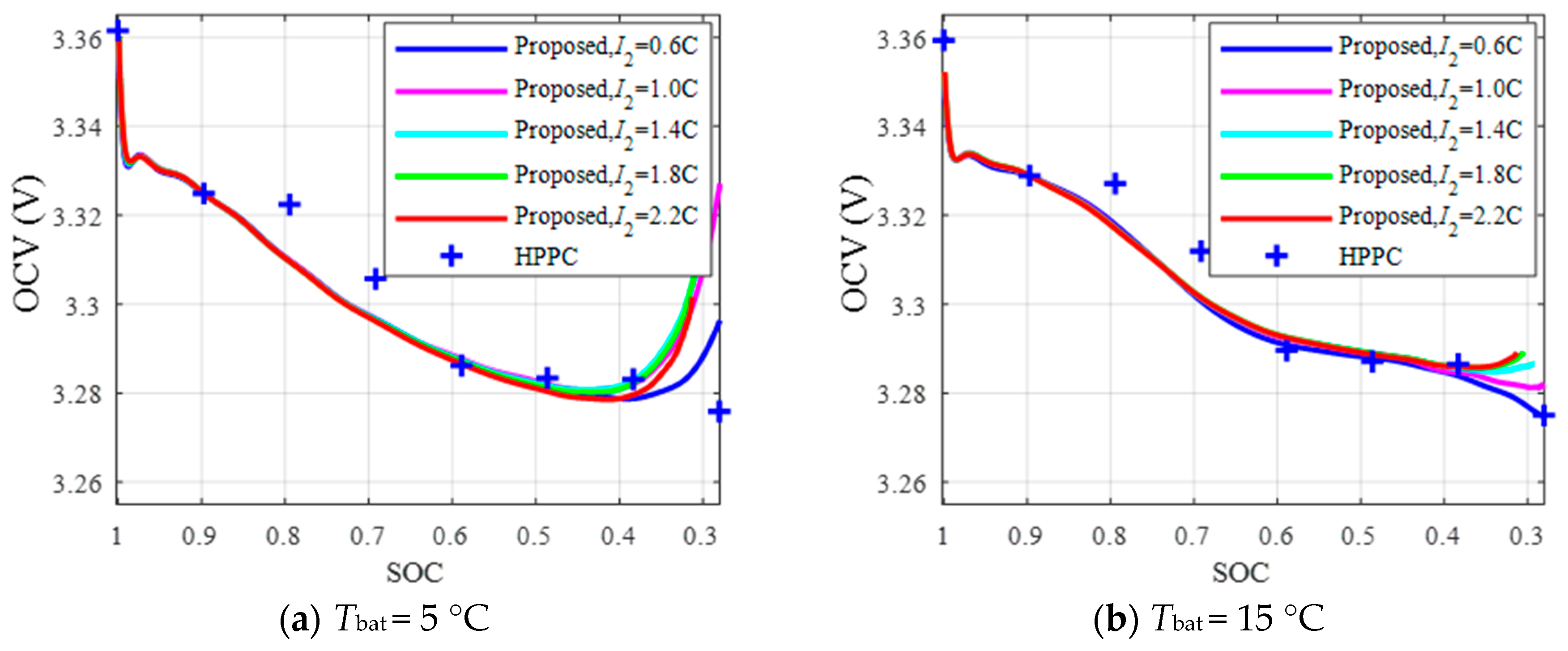
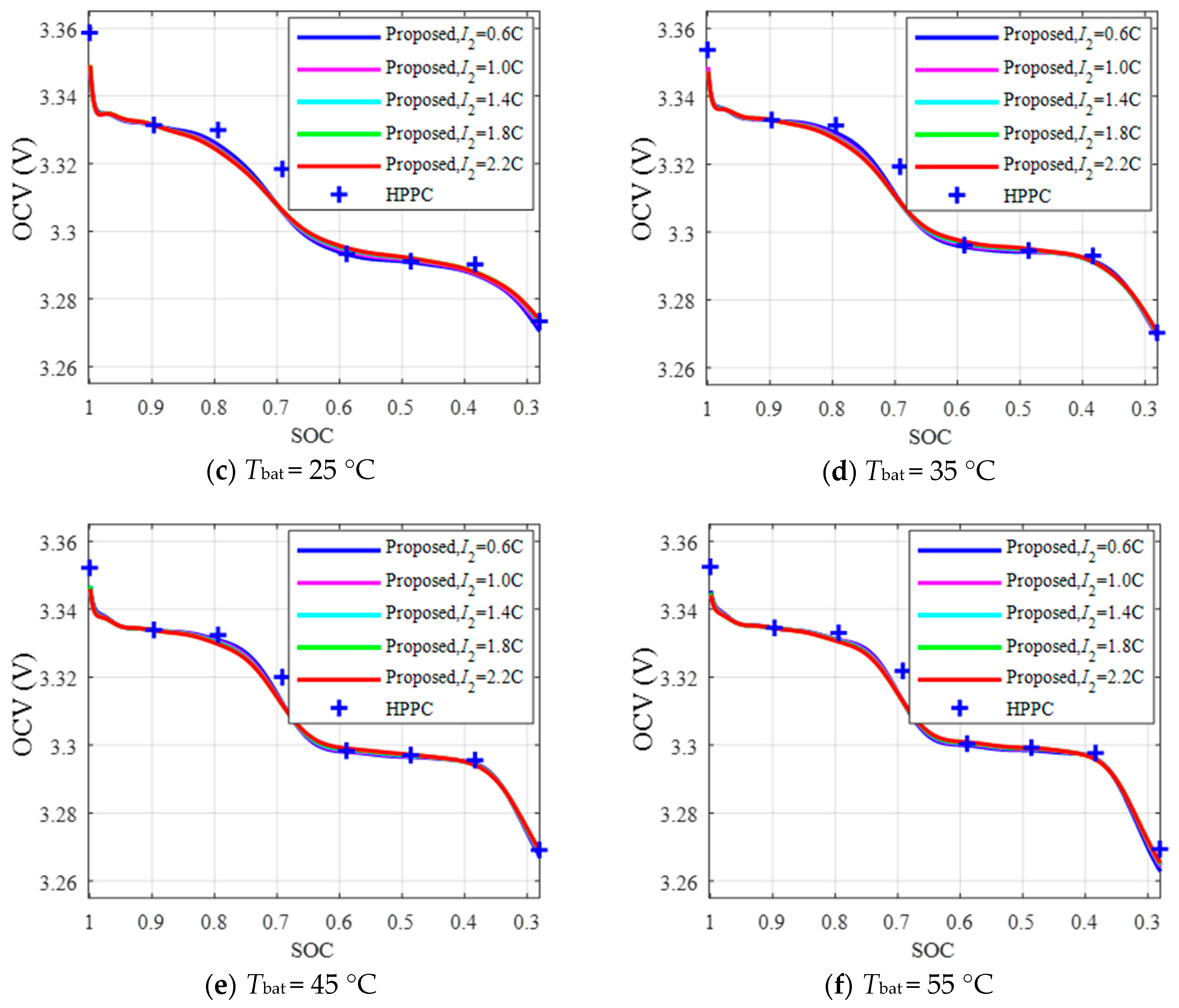
Design of Specific Value of {I1,I2,…,In}
3.2.3. Design of the Specific Value of and Number m
4. Comparison between Different Methods
4.1. Experiments for Method Comparison
4.2. Comparision and Analysis
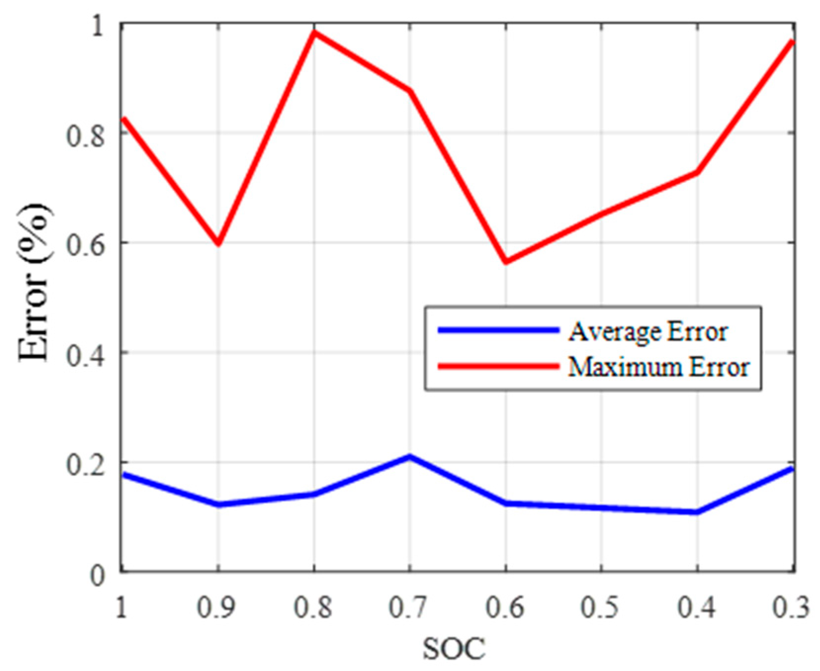
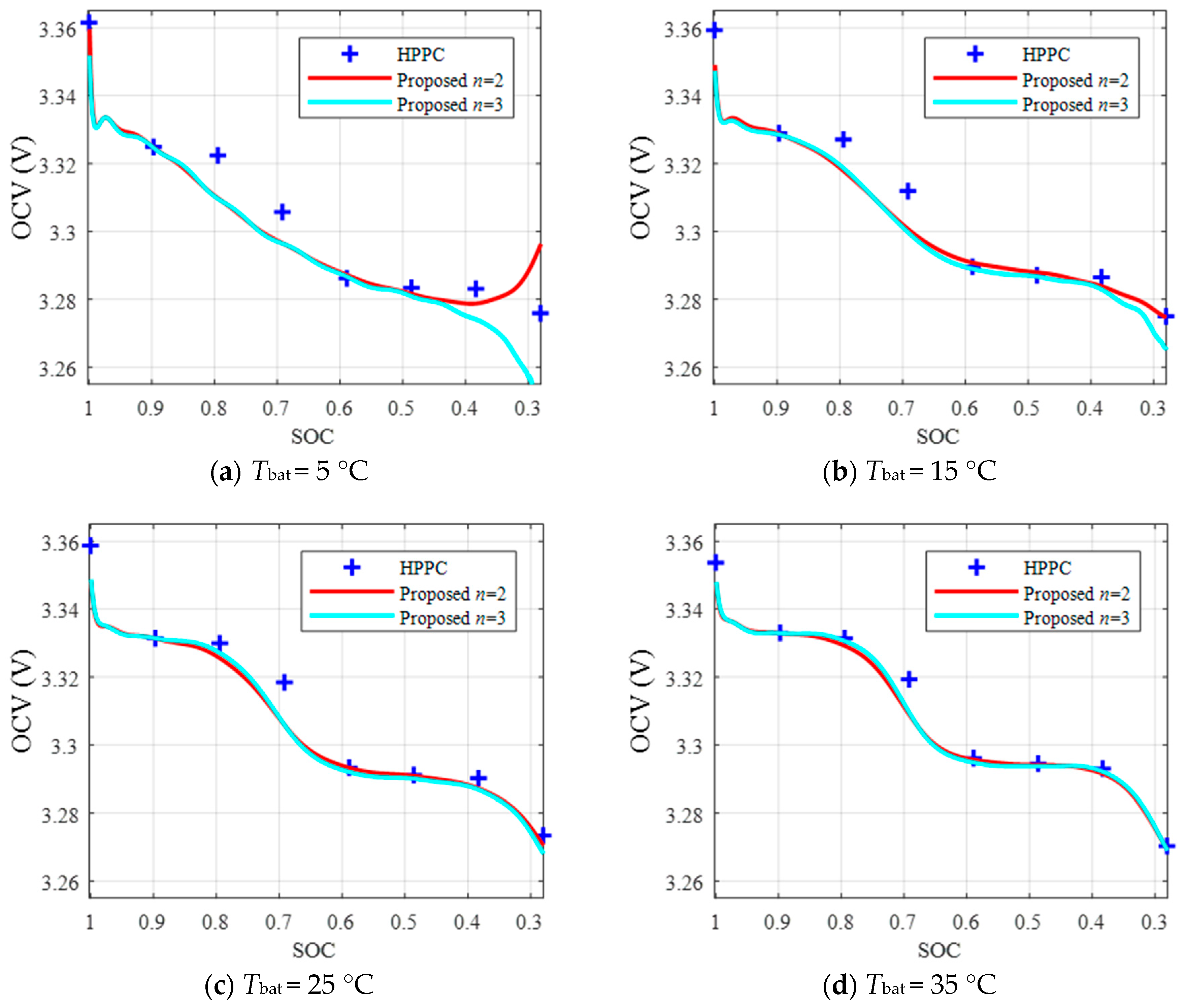
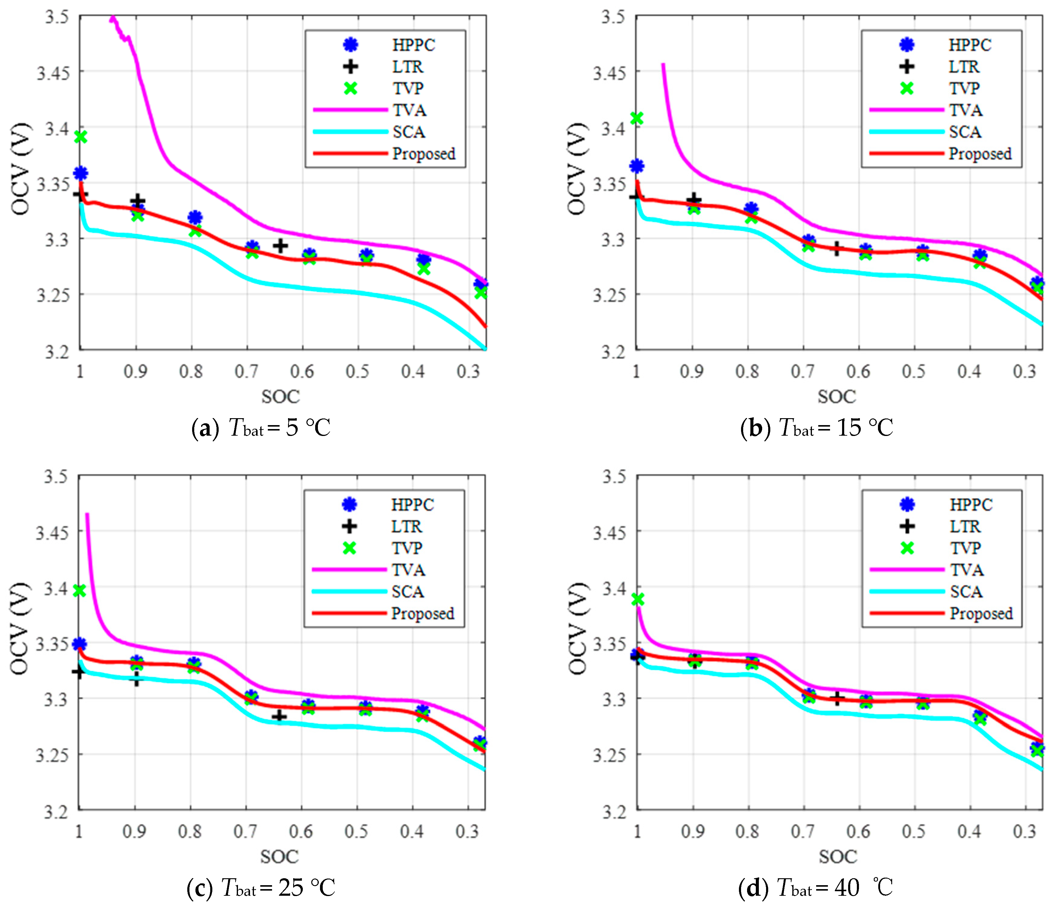
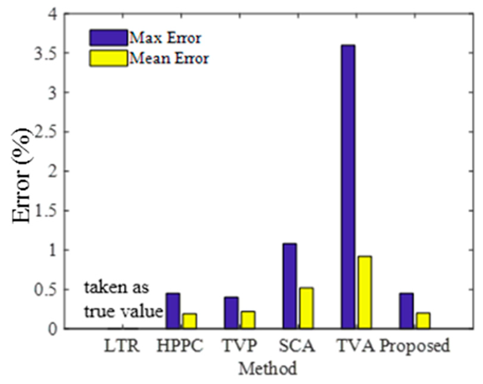
4.2.1. Estimation Accuracy
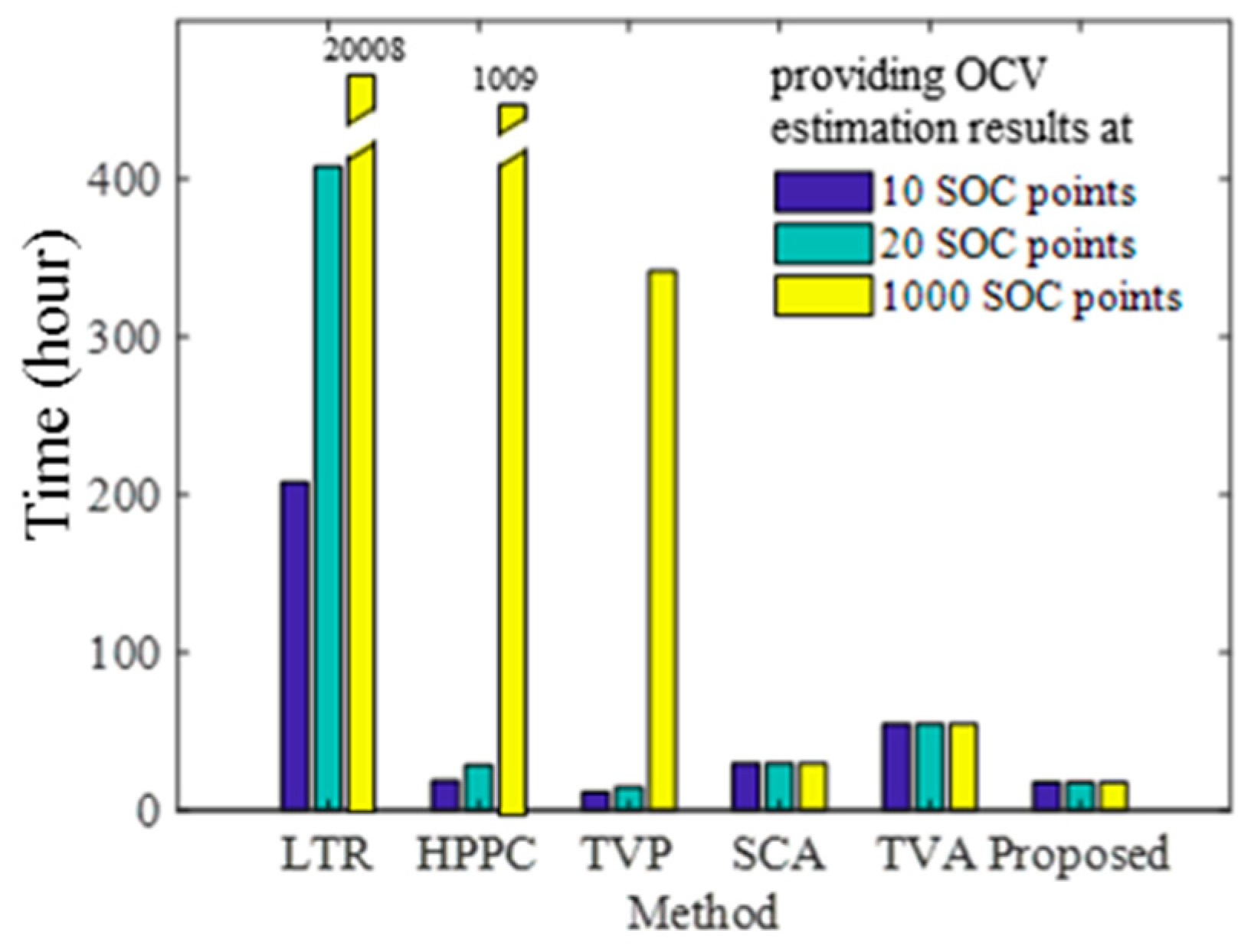
4.2.2. Experimental Time
4.2.3. Other Battery Information
5. Conclusions
Author Contributions
Funding
Conflicts of Interest
Nomenclature
| a | OCV estimation error with large-current experimental data |
| Ah | ampere hour |
| C | C rate, per unit of experimental current |
| CC | constant current |
| CCT | constant current test |
| Cnom | nominal capacity |
| ECM | equivalent circuit model |
| f(I)|SOC,Tj | U–I function at {SOC,Tj} |
| |SOC,Tj | fitted f(I) with large-current experimental data |
| g(Tbat)|SOC,Ii | U–Tbat function at {SOC,Ii} |
| HPPC | hybrid pulse power characterization |
| ICA | incremental capacity analysis |
| I | working current |
| I1, I2, I3, Ii, In | specific experiment current |
| IL | minimum I in working range |
| IH | maximum I in working range |
| LTR | long time rest |
| LPF/C | LiFePO4/Graphite |
| m | number of experimental ambient temperatures |
| n | number of experimental currents |
| NCM/C | Nickel-Cobalt-Manganese/Graphite |
| OCV | open circuit voltage |
| SCA | small-current approximation |
| SOC | state of charge |
| SOCL | minimum SOC in working range |
| SOCH | maximum SOC in working range |
| SOC* | a specific state of charge |
| SOCref | state of charge where OCV is measured |
| t | operation time |
| t0 | start time of the operation |
| T1, T2, Tj, Tm | specific temperature |
| Tij | Tbat when discharging/charging the battery to SOC with I = Ii under Tamb = Tj. |
| ΔT | Tbat changes during operation |
| Tamb | ambient temperature |
| Tbat | battery temperature |
| TbatL | minimum Tbat in working range |
| TbatH | maximum Tbat in working range |
| TVA | terminal voltage average |
| TVP | terminal voltage prediction |
| U | terminal voltage |
| U(I = 0) | terminal voltage when I = 0 in the CCT |
| ΔU | terminal voltage drop |
| VR | voltage relaxation |
| Z | equivalent impedance |
| ^ | estimated value |
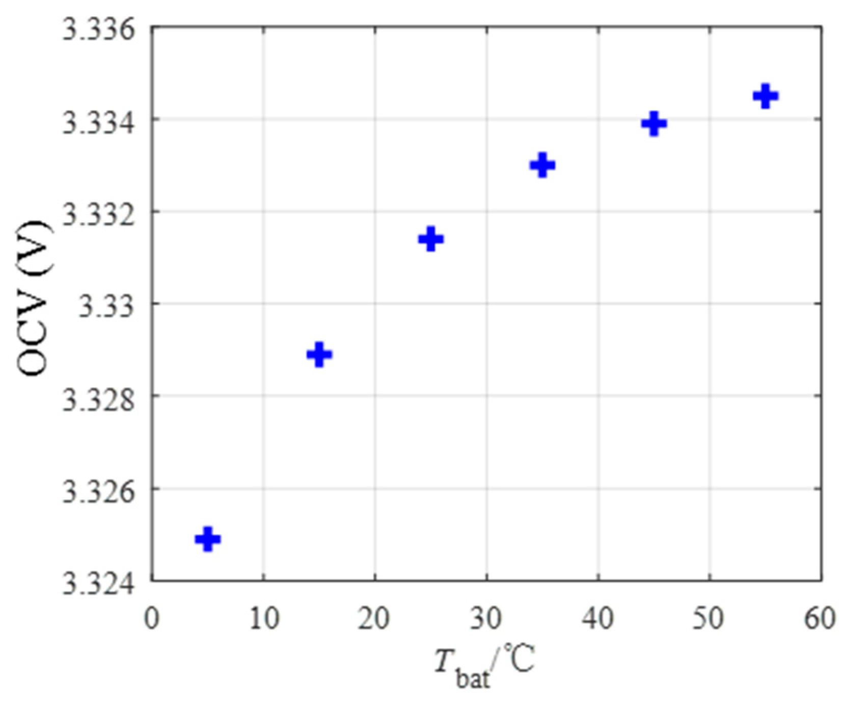
Appendix A: Proof That the U–Tbat Relation Is Continuous and Monotonic
References
- Bard, A.J.; Faulkner, L.R.; Leddy, J.; Zoski, C.G. Electrochemical Methods: Fundamentals and Applications; Wiley: New York, NY, USA, 1980. [Google Scholar]
- Hu, X.; Li, S.; Peng, H. A comparative study of equivalent circuit models for Li-ion batteries. J. Power Sources 2012, 198, 359–367. [Google Scholar] [CrossRef]
- Bernardi, D.; Pawlikowski, E.; Newman, J. A General Energy Balance for Battery Systems. J. Electrochem. Soc. 1985, 132, 5–12. [Google Scholar] [CrossRef]
- Piller, S.; Perrin, M.; Jossen, A. Methods for state-of-charge determination and their applications. J. Power Sources 2001, 96, 113–120. [Google Scholar] [CrossRef]
- Roscher, M.A.; Assfalg, J.; Bohlen, O.S. Detection of Utilizable Capacity Deterioration in Battery Systems. IEEE Trans. Veh. Technol. 2011, 60, 98–103. [Google Scholar] [CrossRef]
- Cassani, P.A.; Williamson, S.S. Design, Testing, and Validation of a Simplified Control Scheme for a Novel Plug-In Hybrid Electric Vehicle Battery Cell Equalizer. IEEE Trans. Ind. Electron. 2010, 57, 3956–3962. [Google Scholar] [CrossRef]
- Jossen, A. Fundamentals of battery dynamics. J. Power Sources 2006, 154, 530–538. [Google Scholar] [CrossRef]
- Chen, M.; Rincon-Mora, G.A. Accurate electrical battery model capable of predicting runtime and I-V conductance. IEEE Trans. Energy Convers. 2006, 21, 504–511. [Google Scholar] [CrossRef]
- Plett, G.L. Sigma-point Kalman filtering for battery management systems of LiPB-based HEV battery packs: Part 1: Introduction and state estimation. J. Power Sources 2006, 161, 1356–1368. [Google Scholar] [CrossRef]
- Yang, J.; Du, C.; Wang, T.; Gao, Y.; Cheng, X.; Zuo, P.; Ma, Y.; Wang, J.; Yin, G.; Xie, J.; et al. Rapid Prediction of the Open-Circuit-Voltage of Lithium Ion Batteries Based on an Effective Voltage Relaxation Model. Energies 2018, 11, 3444. [Google Scholar] [CrossRef]
- Li, Z.; Huang, J.; Liaw, B.Y.; Zhang, J. On state-of-charge determination for lithium-ion batteries. J. Power Sources 2017, 348, 281–301. [Google Scholar] [CrossRef]
- He, Z.; Yang, G.; Lu, L. A Parameter Identification Method for Dynamics of Lithium Iron Phosphate Batteries Based on Step-Change Current Curves and Constant Current Curves. Energies 2016, 9, 444. [Google Scholar] [CrossRef]
- Linden, D.; Reddy, T. Handbook of Batteries, 3rd ed.; McGraw-Hill Companies: New York, NY, USA, 2002; pp. 154–196. ISBN 0-07-135978-8. [Google Scholar]
- Battery Test Manual for Electric Vehicles, Revision 3. Available online: https://inldigitallibrary.inl.gov/sites/STI/STI/6492291.pdf (accessed on 11 May 2019).
- ISO 12405-1. Electrically Propelled Road Vehicles Test Specification for Lithium-ion Traction Battery Packs and Systems. Institution, British Standards, 2011. Available online: https://www.iso.org/standard/51414.html (accessed on 11 May 2019).
- Pop, V.; Bergveld, H.J.; Danilov, D.; Regtien, P.P.; Notten, P.H. Methods for measuring and modelling a battery’s electro-motive force. In Battery Management Systems; Springer: Dordrecht, The Netherlands, 2008. [Google Scholar]
- Pei, L.; Wang, T.; Lu, R.; Zhu, C. Development of a voltage relaxation model for rapid open-circuit voltage prediction in lithium-ion batteries. J. Power Sources 2014, 253, 412–418. [Google Scholar] [CrossRef]
- Pop, V.; Bergveld, H.J.; het Veld, J.O.; Regtien, P.P.; Danilov, D.; Notten, P.H.L. Modeling battery behavior for accurate state-of-charge indication. J. Electrochem. Soc. 2006, 153, A2013–A2022. [Google Scholar] [CrossRef]
- Weng, C.; Sun, J.; Peng, H. A unified open-circuit-voltage model of lithium-ion batteries for state-of-charge estimation and state-of-health monitoring. J. Power Sources 2014, 258, 228–237. [Google Scholar] [CrossRef]
- Ouyang, M.; Chu, Z.; Lu, L.; Li, J.; Han, X.; Feng, X.; Liu, G. Low temperature aging mechanism identification and lithium deposition in a large format lithium iron phosphate battery for different charge profiles. J. Power Sources 2015, 286, 309–320. [Google Scholar] [CrossRef]
- Lu, L.; Han, X.; Li, J.; Hua, J.; Ouyang, M. A review on the key issues for lithium-ion battery management in electric vehicles. J. Power Sources 2013, 226, 272–288. [Google Scholar] [CrossRef]
- Introduction of BMS Products. Available online: http://www.hyperstrong.net/bms.html (accessed on 20 December 2018).
- Chen, Y.; Liu, X.; Yang, G.; Geng, H. An Internal Resistance Estimation Method of Lithium-ion Batteries with Constant Current Tests Considering Thermal Effect. In Proceedings of the IECON 2017 -43rd Annual Conference of the IEEE Industrial Electronics Society, Beijing, China, 29 October–1 November 2017. [Google Scholar]
- Waag, W.; Käbitz, S.; Sauer, D.U. Experimental investigation of the lithium-ion battery impedance characteristic at various conditions and aging states and its influence on the application. Appl. Energy 2013, 102, 885–897. [Google Scholar] [CrossRef]
- Pattipati, B.; Balasingam, B.; Avvari, G.V.; Pattipati, K.R.; Bar-Shalom, Y. Open circuit voltage characterization of lithium-ion batteries. J. Power Sources 2014, 269, 317–333. [Google Scholar] [CrossRef]


| Parameters | Value |
|---|---|
| Type | 26650MP2-Fe |
| Electrode material | LiFePO4/Graphite |
| Nominal capacity/Ah | 3 |
| Maximum constant charging current/C 1 | 2 |
| Maximum constant discharging current/C | 3 |
| I/C 1 | Tamb/°C |
|---|---|
| 0.2/0.6/1.0/1.4/1.8/2.2 | 5/15/25/35/45/55 |
| Methods | Error Max Mean | Experimental Time 1/hour Estimation Results at 10/20/1000 SOC Points | Other Information | |||
|---|---|---|---|---|---|---|
| LTR | taken as true value | 208 | 408 | 20008 | Impedance | |
| HPPC | 0.45% | 0.19% | 19 | 29 | 1009 | Impedance |
| TVP | 0.40% | 0.22% | 11.7 | 15 | 341.7 | Impedance |
| SCA | 1.08% | 0.52% | 30 | 30 | 30 | capacity with small-current conditions, ICA information |
| TVA | 3.60% | 0.92% | 55 | 55 | 55 | capacity/resistance with small-current conditions, ICA information |
| Proposed | 0.45% | 0.20% | 18 | 18 | 18 | capacity/resistance with normal-current condition, thermal characteristics, ICA information |
© 2019 by the authors. Licensee MDPI, Basel, Switzerland. This article is an open access article distributed under the terms and conditions of the Creative Commons Attribution (CC BY) license (http://creativecommons.org/licenses/by/4.0/).
Share and Cite
Chen, Y.; Yang, G.; Liu, X.; He, Z. A Time-Efficient and Accurate Open Circuit Voltage Estimation Method for Lithium-Ion Batteries. Energies 2019, 12, 1803. https://doi.org/10.3390/en12091803
Chen Y, Yang G, Liu X, He Z. A Time-Efficient and Accurate Open Circuit Voltage Estimation Method for Lithium-Ion Batteries. Energies. 2019; 12(9):1803. https://doi.org/10.3390/en12091803
Chicago/Turabian StyleChen, Yingjie, Geng Yang, Xu Liu, and Zhichao He. 2019. "A Time-Efficient and Accurate Open Circuit Voltage Estimation Method for Lithium-Ion Batteries" Energies 12, no. 9: 1803. https://doi.org/10.3390/en12091803