Wavelet Packet Decomposition for IEC Compliant Assessment of Harmonics under Stationary and Fluctuating Conditions

Abstract

This paper presents the validation and characterization of a wavelet based decomposition method for the assessment of harmonic distortion in power systems, under stationary and non-stationary conditions. It uses Wavelet Packet Decomposition with Butterworth Infinite Impulse Response filters and a decomposition structure, which allows the measurement of both odd and even harmonics, up to the 63rd order, fully compliant with the requirements of the IEC 61000-4-7 standard. The method is shown to fulfil the IEC accuracy requirements for stationary harmonics, obtaining the same accuracy even under fluctuating conditions. Then, it is validated using simulated signals with real harmonic content. The proposed method is proven to be fully equivalent to Fourier analysis under stationary conditions, being often more accurate. Under non-stationary conditions, instead, it provides significantly higher accuracy, while the IEC strategy produces large errors. Lastly, the method is tested with real current and voltage signals, measured in conditions of high harmonic distortion. The proposed strategy provides a method with superior performance for fluctuating harmonics, but at the same time IEC compliant under stationary conditions.

1. Introduction

The fast evolution of electrical and electronic technologies is generating an exponential growth in the use of non-linear loads, such as switch-mode power supplies, electronic lighting ballasts [1], and other harmonic sources whose penetration can be expected to increase substantially in the future [2]. Harmonic distortions coming from new-generation sources and loads are generally larger and less regular than those due to traditional sources and loads, making power and energy more difficult to measure [3,4]. International standards have been developed to define acceptable limits and suitable measurements techniques for power systems’ harmonics, e.g., [5,6]. Fourier spectral analysis is the most widely used approach for the evaluation of the harmonic content in power systems, due to its excellent accuracy under stationary conditions. This choice is reflected in the IEC 61000-4-7 [5] standard, which defines harmonics measurements and instrumentation requirements. This standard proposes the use of the Fast Fourier Transform (FFT), a fast and efficient algorithm for performing the Discrete Fourier Transform (DFT). Although the DFT is valid under general conditions, it is well known that limitations arise when it is applied to non-stationary signals, which is the normal situation in modern power systems. When fluctuating harmonics are analyzed with a DFT, the energy contained in the harmonics is distributed across the spectrum, affecting the accuracy [7]. For this reason, the IEC 61000-4-7 standard proposes a grouping strategy in order to improve the accuracy in non-stationary conditions and, at the same time, explicitly mentions the possibility to employ more advanced processing tools. During the last few years, alternatives to DFT have been proposed in the literature. A common workaround is to use the Short Time Fourier Transform (STFT), which assumes the signal to be piecewise stationary, but other methods have been suggested as well [8]. Among them, there is Wavelet Transform (WT), typically in the form of Discrete Wavelet Transform (DWT). The main advantage of DWT is that, while DFT requires a stationary, perfectly periodic sinusoidal signal to work properly, this is not a requirement for DWT. This signal processing tool has a wide range of applications, including power systems, where it proved to be extremely useful in signal denoising, short time predictions, fault detection, and energy management [9,10,11,12,13,14], as well as for Power Quality [15,16,17,18,19]. From WT, Wavelet Packet Decomposition (WPD) was derived, generalizing the link between wavelets and Multiresolution Analysis (MRA). Thanks to the uniform frequency bands that can be obtained with WPD, its application in Power Quality has been proposed for power calculation [20,21] and harmonic measurements [22,23,24]. However, the WPD harmonic analyses proposed in the literature do not look complete from the point of view of compliance with international standards and capabilities under stationary conditions, as will be discussed in Section 2.

To complete the current scenario, this paper presents a WPD method for a full harmonic analysis, in contrast with the valuable, but partial work developed in recent years, e.g., [22,23,24,25]. The proposed method takes advantage of the superior performance of WPD with fluctuating harmonics with respect to Fourier analysis. On the other hand, it is for the first time compliant with the IEC 61000-4-7 standard. This result, never achieved before, is possible thanks to the accurate selection of the filtering implementation and to the uniform frequency bandwidth division of WPD, as studied by the authors in [26]. To assess the method’s implementation and validate its superior performance within the IEC standard requirements, several voltage signals with known harmonic content, both in stationary and fluctuating conditions, were tested. The accurate assessment of individual harmonic values was the main focus of the proposed method, and therefore, they were the objective of the validation. Other indices, like for instance Total Harmonic Distortion (THD), were not considered since they are the result of a further processing stage that can be performed in the same way as for FFT, as explained in Section 2.2. In Section 4.4, a comparison of the computational effort is provided, and finally, in Section 5, the method is tested with real voltage and current signals measured in a high harmonic distortion environment.

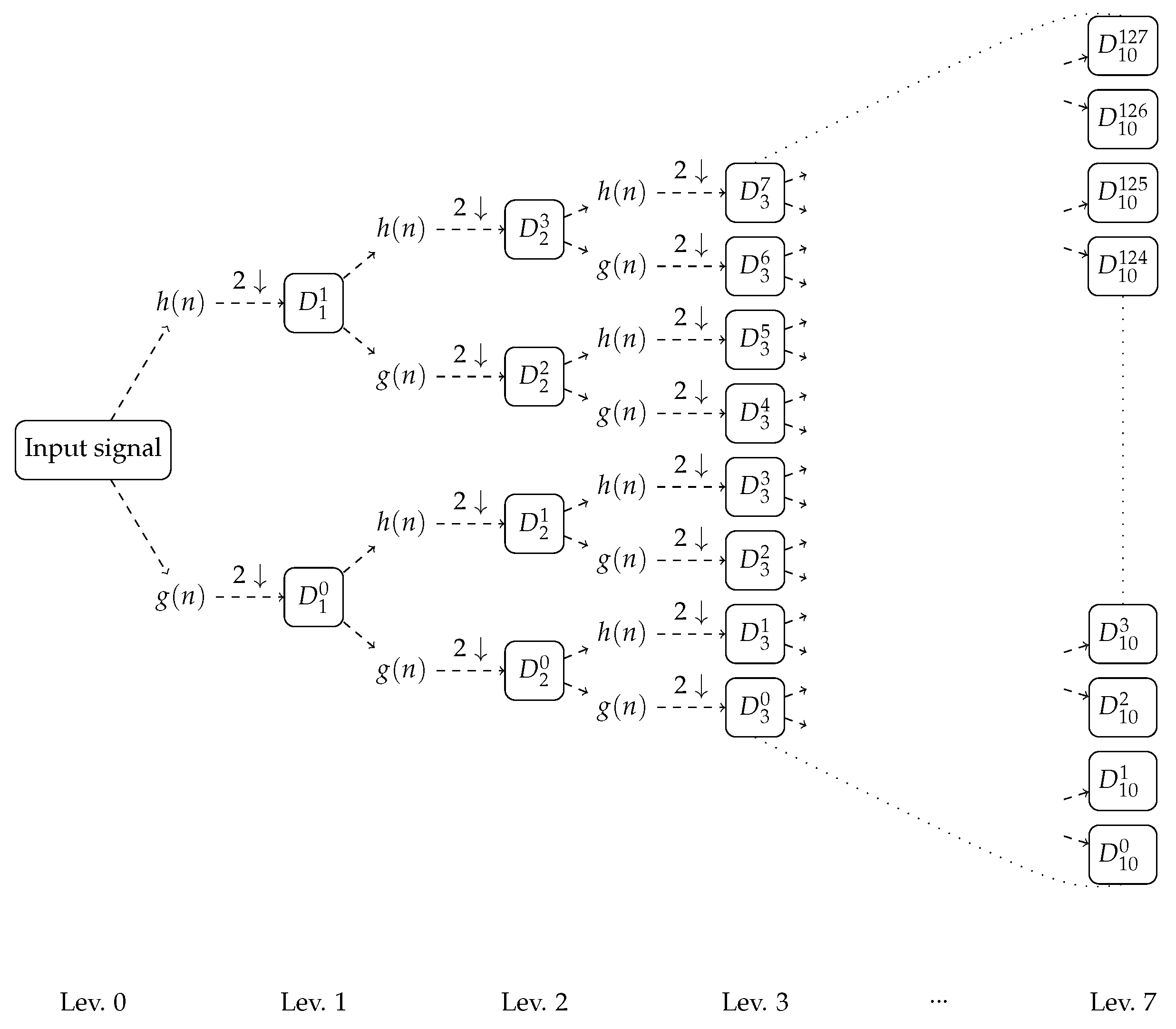
2. The Proposed WPD Method

2.1. Wavelet Transforms in Power Systems

WT is a mathematical transform that provides a representation of a function by a series of orthonormal functions, generated by scaling and translating a wavelet. It is particularly powerful in the measurement of the time-frequency variations of spectral components, but not suitable for power harmonics analysis because of the non-uniform frequency bands obtained. WPD is an extension of WT where the frequency axis is divided into equally wide intervals, instead of the traditional division in dyadic intervals, whose sizes have an exponential growth [27]. The advantage is that, with an accurate selection of the sampling frequency and the decomposition structure, it can lead to uniform frequency bands of the desired size and can therefore be employed for harmonics analysis. Previous works on WPD based algorithms for harmonics analysis can be found in the literature, but up to this moment, no IEC compliant approach, with complete harmonic analysis, has been proposed. Hamid et al. presented in [21] a WPD method for Root Mean Squared (RMS) and power measurements, from which harmonic distortion can be obtained. However, with this approach, only odd harmonics can be evaluated, and the wide frequency bands that can be obtained are not compliant with IEC standards. Eren et al. proposed a decomposition scheme in [22], but again, only bands centered in odd harmonics were taken into account. Moreover, results were shown only up to the seventh order. A more refined strategy was proposed by Diego and Barros in [24], where the 50 $\mathrm{Hz}$ wide frequency bands were compatible with IEC 61000-4-7 [5], but the decomposition was performed only up to the 15th order, far from compliance with the IEC standards.

Additionally, a major drawback of WPD based algorithms is their difficulty to compete with FFT in terms of computational speed. The FFT algorithm is the result of many years of developments and advances of Fourier analysis, while newly proposed methods (such as WPD) are not yet optimized for high performances. However, this gap is reducing, thanks to the constant increase in available computational power and the possibility of hardware implementation. In [23], it was shown that WPD can be efficiently implemented and be employed online for harmonics analysis. However, although the work showed the feasibility of online measurements, the same limitations on the results were found, i.e., the evaluation of only odd harmonics, limited total bandwidth (only up to 15th order), and too wide frequency bands (even harmonics contributions were included in the odd ones).

WPD algorithms continue to be interesting for power system researchers, as suggested by recent works [20,23], but in order to move forward and make WPD a feasible and better alternative to DFT, a complete algorithm for harmonic assessment must be designed. Modern power systems, with the increasing presence of non-linear loads, require a method compatible with the IEC standards, able to measure not only odd harmonics, but also even harmonics, and up to the highest possible order.

2.2. Characteristics of the Proposed Method

The past limitations of WPD arose from the difficulty of adjusting the algorithm to the constraints given in the IEC 61000-4-7 standard, which is not trivial. Among these constraints, there are: a fixed rectangular sampling window of 10 cycles of the fundamental (200 $\mathrm{m}$$\mathrm{s}$ at 50 $\mathrm{Hz}$), frequency bands of 50 $\mathrm{Hz}$ centered in integer multiples of the fundamental (both even and odd), a bandwidth up to the 50th harmonic order (2500 $\mathrm{Hz}$), and mainly, the fulfillment of the accuracy requirements for the stationary case. Therefore, the implementation of an IEC compliant algorithm is not just an extension of previous studies, since it requires overcoming the previous limitations and keeping the accuracy within the prescribed limits.

In this paper, it is shown that this can be achieved by an accurate study of the WPD implementation. The novel algorithm hereafter presented is the continuation of the work performed by the authors in [26], where a detailed study was conducted to define a methodology for the selection of the most suitable filter and convolution technique for WPD applied to power systems’ harmonics. The methodology proposed in [26] is here employed to develop and characterize a complete measurement method. In order to obtain the IEC frequency bands, up to at least the 50th order, a sampling rate of 6400 $\mathrm{Hz}$ is necessary, and seven levels of decomposition must be implemented. These necessary features set high requirements on the frequency selectivity of the decomposition filters. The work performed in [26] showed that a maximally-flat Butterworth Infinite Impulse Response (IIR) filter of order 29 was the most suitable choice, and for this reason, it was employed in this paper as the mother wavelet. Its superior behavior in frequency selectivity, number of coefficients, and spectral leakage under realistic conditions, compared with traditional mother wavelet functions (e.g., db20, db10, Vaidyanathan, etc.) provides the high level of accuracy required to comply with the IEC standards in both stationary and non-stationary conditions. It must be noted that, although IIR filters have a non-linear phase, it does not represent a problem because the purpose of the method is to extract the RMS content of each frequency band, and the convolution technique presented in [26] allows preserving this information even with non-linear phase filtering.

In the following, the filtering procedure at each node of the decomposition tree is explained: the input signal f is recursively convolved by a pair of Quadrature Mirror Filters (QMFs), high pass and low pass filters ($h\left(n\right)$ and $g\left(n\right)$, respectively), and then, the filtered signals are downsampled by a factor of two, taking into account that the employed filters are half band filters (see Equations (1) and (2)). Thus, the high pass and low pass QMFs used were obtained from the corresponding IIR Butterworth filter of order 29, as discussed before. This WPD scheme was designed and implemented using MATLAB, allowing the authors to speed up the validation and testing procedure under realistic input conditions, i.e., with the evaluation of real voltage waveforms. The following equations describe the basic filtering stage of the WPD method, in which the wavelet coefficients at level l, node i, are obtained from the convolution of the input signal at the previous level with the filters’ coefficients and subsequent downsampling.

$$\begin{array}{c}\hfill D_{\mathrm{l}}^{2\mathrm{i}}\left(k\right)=\sum _{n}g\left(n\right)D_{\mathrm{l}-1}^{\mathrm{i}}(2k-n)\end{array}$$

(1)

$$\begin{array}{c}\hfill D_{\mathrm{l}}^{2\mathrm{i}+1}\left(k\right)=\sum _{n}h\left(n\right)D_{\mathrm{l}-1}^{\mathrm{i}}(2k-n)\end{array}$$

(2)

where $i=0,1,\dots ,2(l-1)-1$, and $h\left(n\right)$ and $g\left(n\right)$ are the high pass and low pass filter coefficients, respectively. In this regard, Figure 1 shows the decomposition tree scheme employed.

Table 1. Decomposition tree summary.

Level Number	Number of Nodes	Samples/Node	Δt (ms)	Bw/Node (Hz)
1	2	640	0.312	1600
2	4	320	0.625	800
3	8	160	1.250	400
4	16	80	2.500	200
5	32	40	5.000	100
6	64	20	10.000	50
7	128	10	20.000	25
7*	128/2 = 64	10 + 10 = 20	N/A	25 + 25 = 50

summarizes the characteristics of the decomposition structure at each node, including information about the number of nodes per level, samples per node, effective time resolution, and bandwidth for every node at each level.

It is possible to observe that nodes at the seventh decomposition level have a bandwidth of 25 $\mathrm{Hz}$. The required 50 $\mathrm{Hz}$ bands were obtained by a two-nodal-grouping (7*, last level in Table 1). Aggregated RMS harmonic values are derived from individual node content as follows [15]:

$$x_{rms}(j,p+q)=\sqrt{\frac{{\sum }_k{(d_{j,k}^p)}^2+{\sum }_k{(d_{j,k}^q)}^2}{N}}$$

(3)

where p and q are the two grouped nodes, N the total number of data, k the index counter, and j the level at which the RMS calculation is performed. In order to obtain the correct IEC bands, the grouping must satisfy: $q=p+1,p=2,4,6,\dots$ (the first node is discarded).

Thanks to this two-nodal-grouping, each band corresponded exactly to an IEC harmonic group, and therefore, any further processing stage, e.g., THD calculation or time aggregation according to IEC 61000-4-30, is perfectly possible. The algorithm was indeed designed to represent an alternative to FFT for power quality analyzers, assuming sampled values as input and producing compliant individual harmonic values as output. As a result, the method did not have any additional requirements than those of FFT.

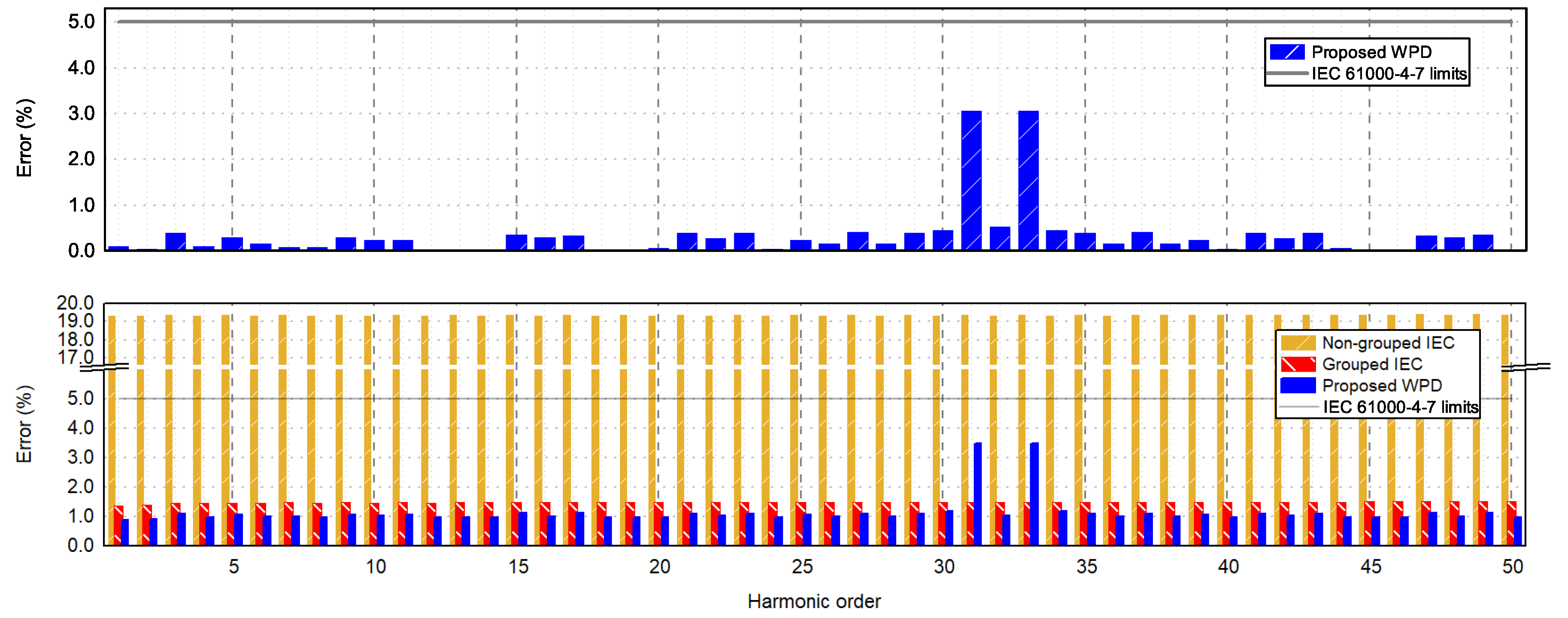
3. Compliance with IEC Accuracy Requirements

This section presents a test of accuracy, showing that the proposed method fulfills the IEC precision requirements for the stationary case and overperforms the IEC standard method for the non-stationary case.

IEC 61000-4-7 prescribes, for Class I accuracy, a maximum error of 5% in the evaluation of harmonic components, in case of single frequency and steady-state signals. In order to test the compliance of the proposed method, fifty steady-state signals $u_{\mathrm{i}}\left(t\right)$, of single harmonic frequency ranging from harmonic order one to 50, were generated with a MATLAB script and subsequently analyzed using both the IEC method and the proposed WPD method. The input signals have the following expression:

$$u_{\mathrm{i}}\left(t\right)=100\sqrt{2}sin\left(i2\pi f_{0}t\right)$$

(4)

where i is the ith test containing the ith pure tone, $f_0$ is the power frequency (50 $\mathrm{Hz}$), and t is the time.

The top graph in Figure 2 shows the errors obtained with the proposed method for each ith harmonic order, with respect to the expected values, which in this case was always 100. It can be seen that the errors were well below the limit for Class I instruments for every harmonic order. The slightly higher errors for order 31st and 33rd were due to an intrinsic characteristic of WPD, which affected the central decomposition bands, as explained in [26]. This, however, did not compromise the accuracy, and compliance with IEC 61000-4-7 was proven.

The same test was repeated for non-stationary single frequency signals. To obtain non-stationary signals, the fluctuation pattern proposed in IEC 61000-4-7 Annex C.3 was employed, i.e., a reduction of the RMS of the signal from 100% to 20% at $t=85 \mathrm{m}\mathrm{s}$ in a 200 $\mathrm{m}$$\mathrm{s}$ window. Since FFT is not suitable for measuring fluctuating harmonics, the standard proposes a grouping strategy, where the FFT bins are summed into harmonic groups to reduce the uncertainty. However, no accuracy limits are prescribed for this scenario. The bottom graph in Figure 2 shows the errors obtained in the case of fluctuating signals using the conventional FFT, the grouped IEC strategy, and the proposed WPD method. It can be seen that the conventional FFT produced errors of the order of 20%, while the IEC grouping strategy allowed a reduction of the error below the 5% limit. In this case, the proposed WPD method further reduced the error, for every order but 31 and 33, never exceeding the IEC stationary-state limits. The proposed method was therefore equally valid as the grouped FFT for single frequency signals, both stationary and fluctuating, and significantly superior to standard FFT, as expected.

4. Validation of the Method

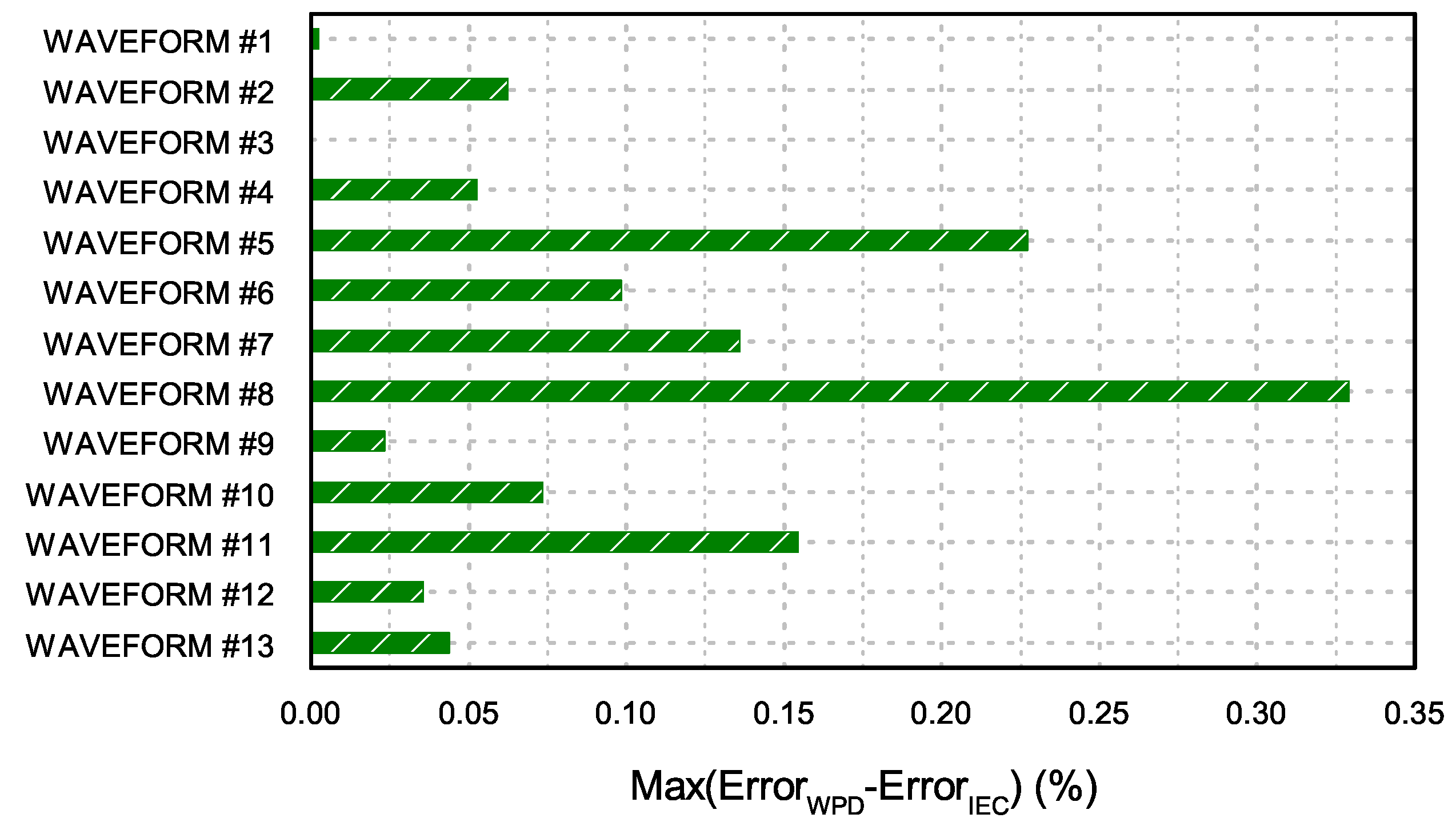
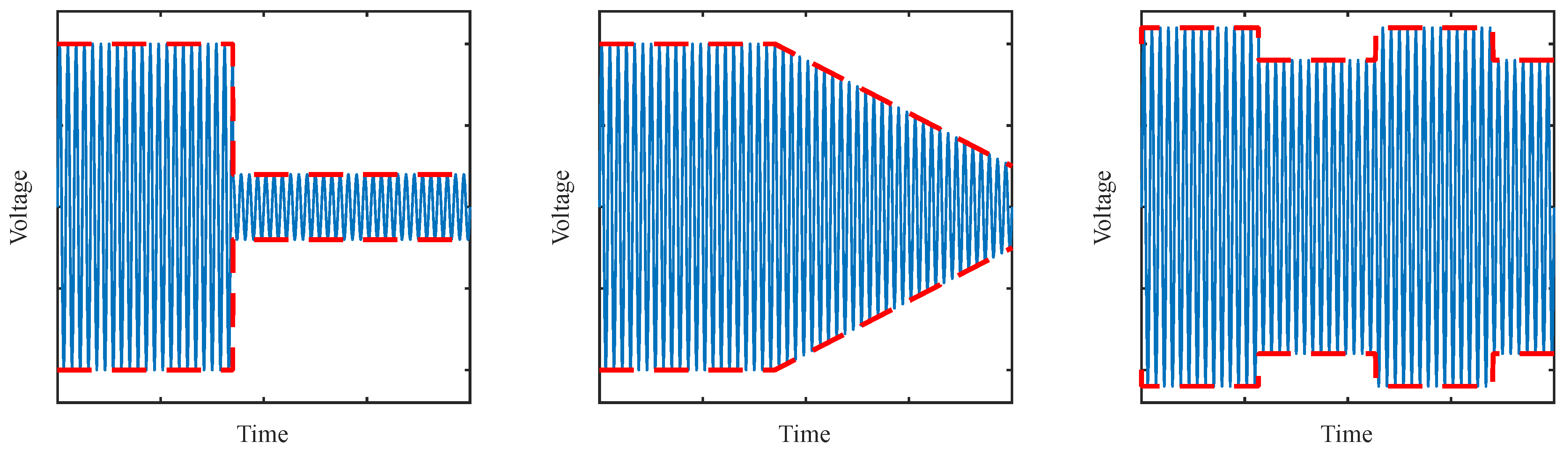
The validation of the method required a more complex harmonic content than single frequency signals. Moreover, in order to be able to assess the accuracy of the method and compare it with the accuracy of Fourier analysis, the true harmonic content of the signals needed to be known a priori, i.e., synthetic signals must be employed. For this reason, realistic signals were generated, starting from the National Physics Laboratory (NPL) Power Quality Waveform Library [28], a public repository of waveforms with known harmonic content, representative of voltage signals found in the grid or used for calibration of equipment. This approach allowed obtaining waveforms whose true harmonic content was known and, at the same time, was realistic harmonic content.

4.1. Test Waveforms

The 13 employed waveforms are presented in

Table 2. Validation test waveforms, taken from [28], showing the total number of harmonic components included n, the most intense harmonic order H, and the calculated THD.

ID	Description	n	H	THD (%)
1	IEC 61000-3-2 voltage limits for the power amplifier	38	3	1.26
2	Voltage waveform for an accounting operation building	4	5	2.80
3	Voltage waveform for an apartment building	6	5	1.95
4	Voltage waveform for a commercial and residential load	3	5	2.44
5	Voltage waveform of fluorescent lights with electronic ballast	5	5	3.74
6	Voltage waveform of fluorescent lights with magnetic ballast	3	5	2.69
7	Voltage waveform for an industrial and residential load	3	5	3.00
8	Possible limits of voltage harmonics of a single phase feeder	49	3	6.72
9	Voltage waveform for a machining plant	4	5	2.00
10	Voltage waveform for a residential load	3	5	2.55
11	Square wave	24	3	47.30
12	Voltage waveform for a supermarket	4	5	2.42
13	Voltage waveform for a welded pipes plant	4	5	2.40

. It was decided to employ all the waveforms of the NPL library coming from direct measurements in the grid (11), together with two synthetic waveforms, to further test the method. The synthetic waveforms were a square wave, allowing testing harmonic contents up to the 49th order, and a waveform whose harmonic content was created using IEC 61000-3-2:2000 limits for harmonic voltage emissions [28]. In each case, the power frequency was 50 $\mathrm{Hz}$, so the duration of the test waveform was 200 $\mathrm{m}$$\mathrm{s}$, as prescribed in IEC 61000-4-7, while the RMS amplitude of the fundamental components was 230 $\mathrm{V}$. Table 2 also shows the THD factors calculated from the nominal harmonic content values reported in [28]. For the study of the non-stationary case, the following modulation patterns were applied to the test waveforms:

• Constant modulation: instantaneous reduction of the amplitude from 100% to 20%, 85 $\mathrm{m}$$\mathrm{s}$ after the beginning of the signal. This is the modulation proposed in IEC 61000-4-7.
• Linear modulation: amplitude linearly reduced from 100% to 75% in the last 115 $\mathrm{m}$$\mathrm{s}$ of the signal. This modulation represents a motor start.
• Rectangular modulation: flicker-type modulation of 5% amplitude and $8.8$ $\mathrm{Hz}$ modulation frequency.

The last two modulations were considered to provide a more reliable validation, since they could be realistically found in the grid, in the case of the connection of large loads or in the case of flicker [29]. More information about the modulation patterns is given in Section 4.3.

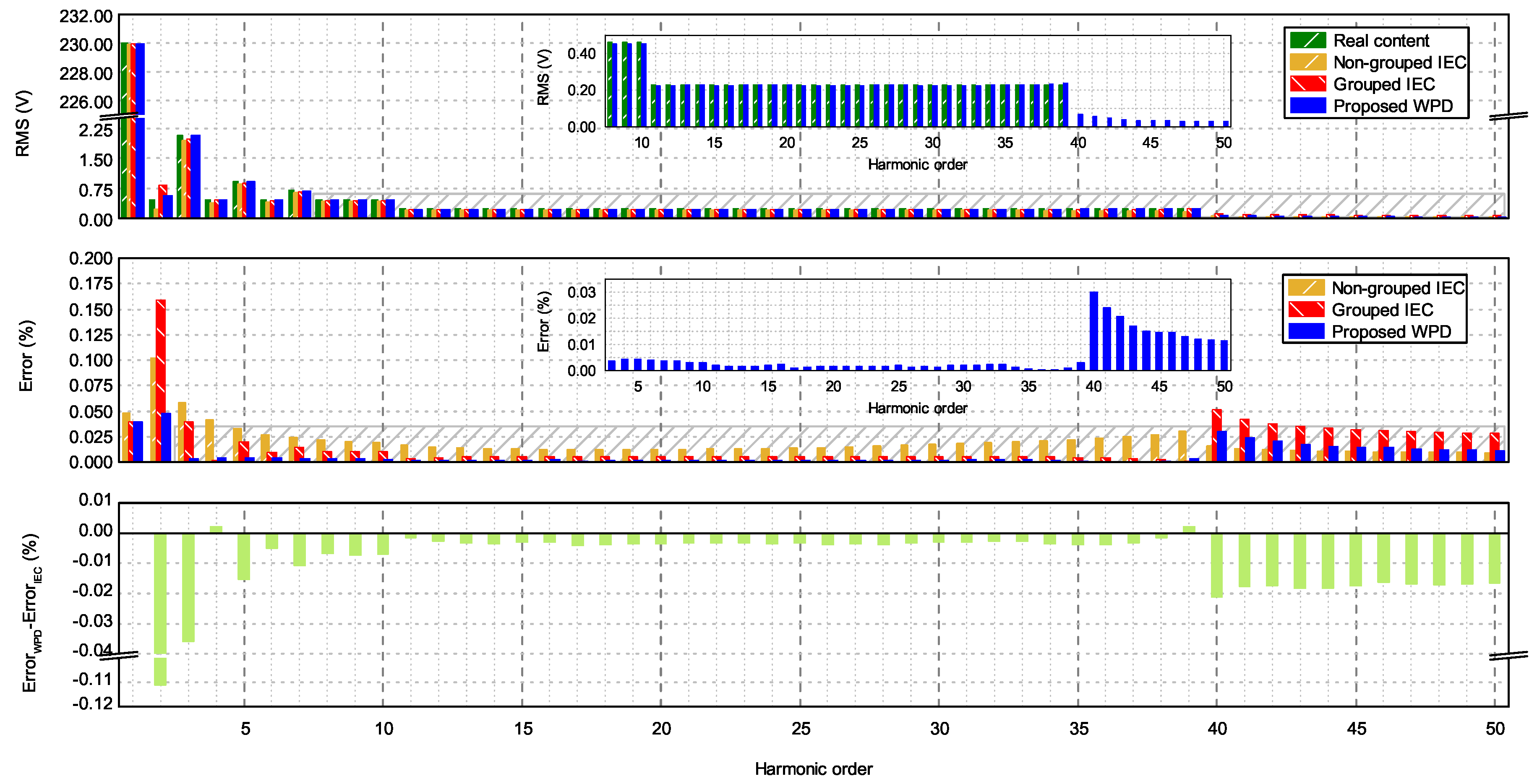
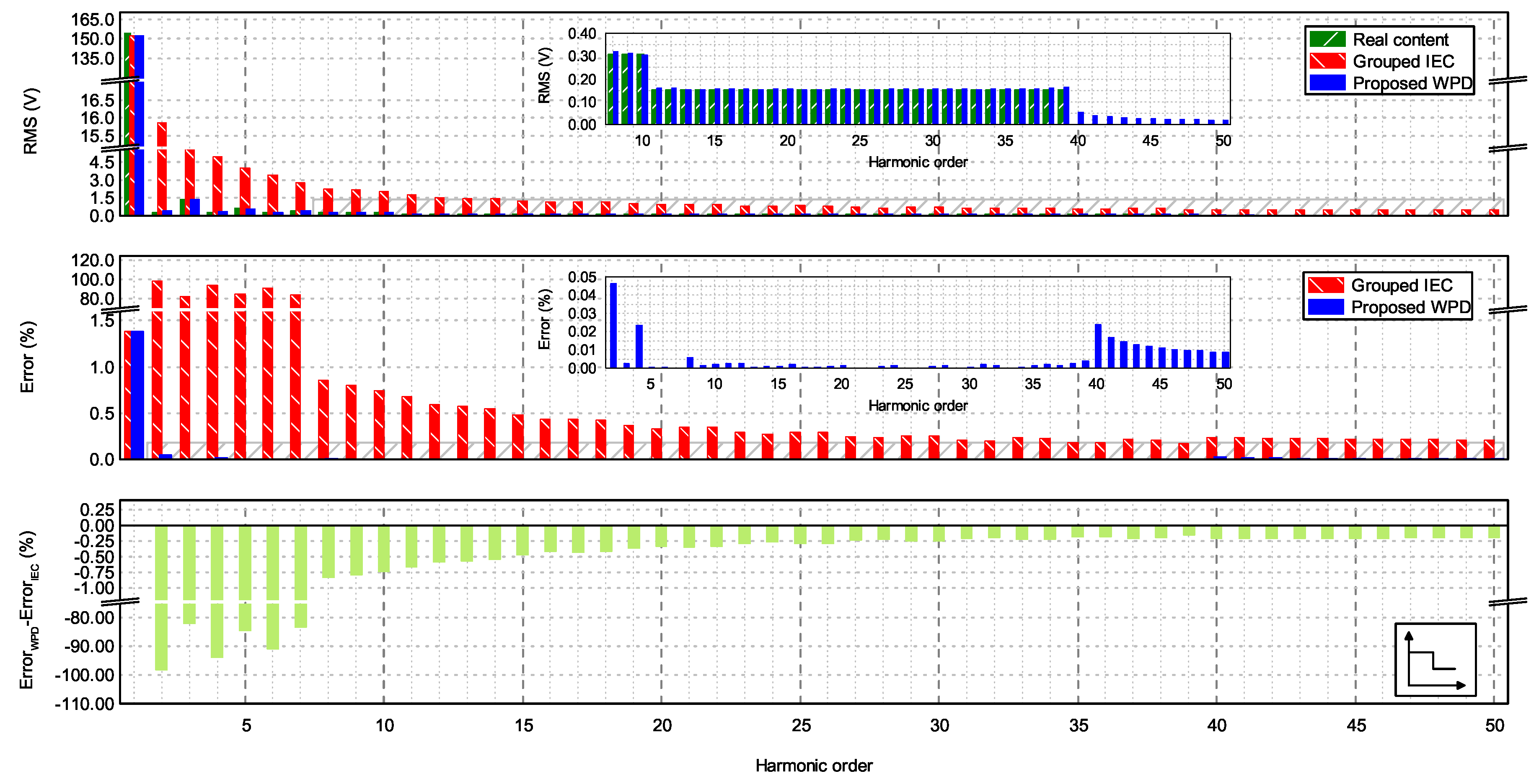
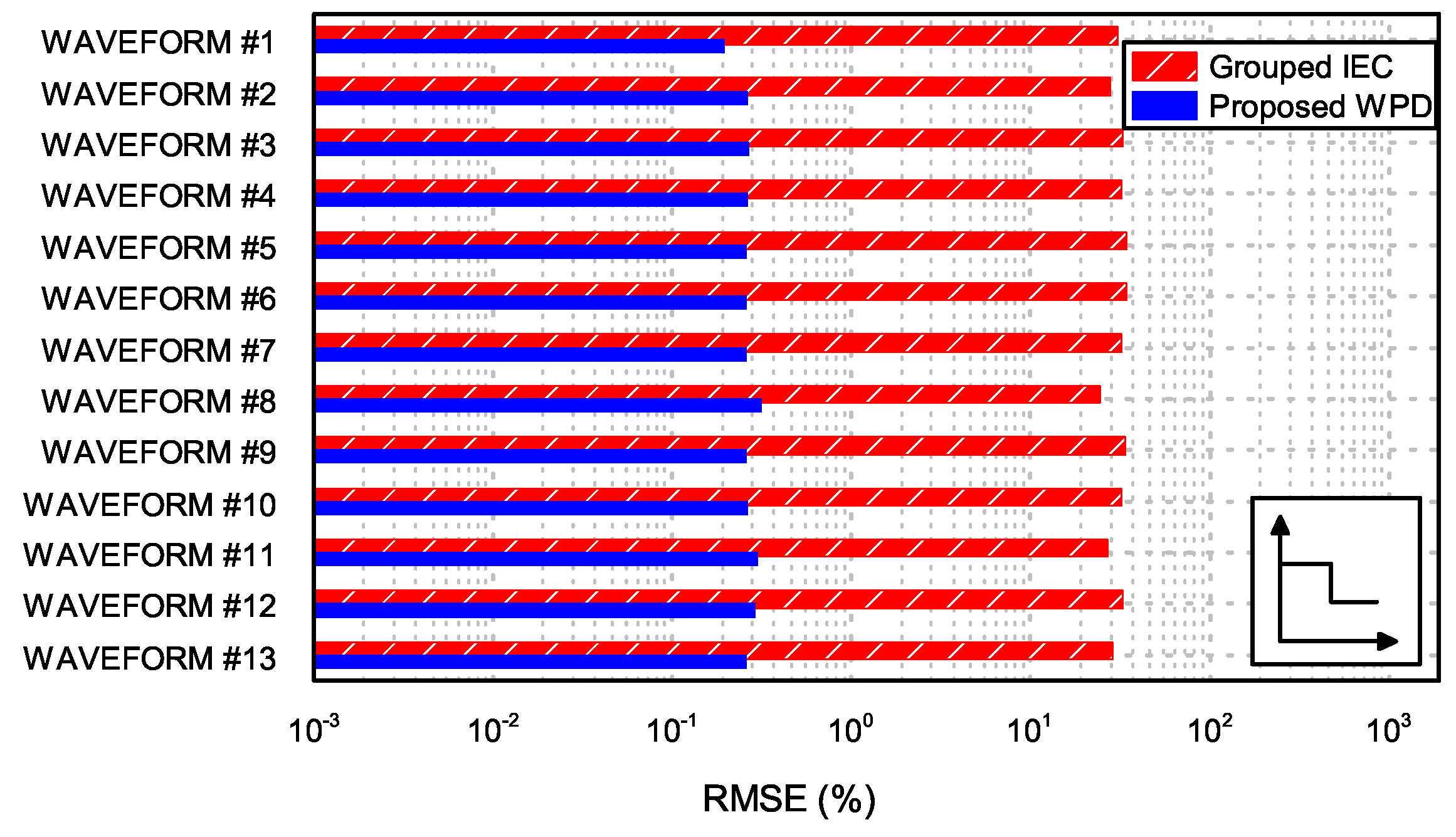
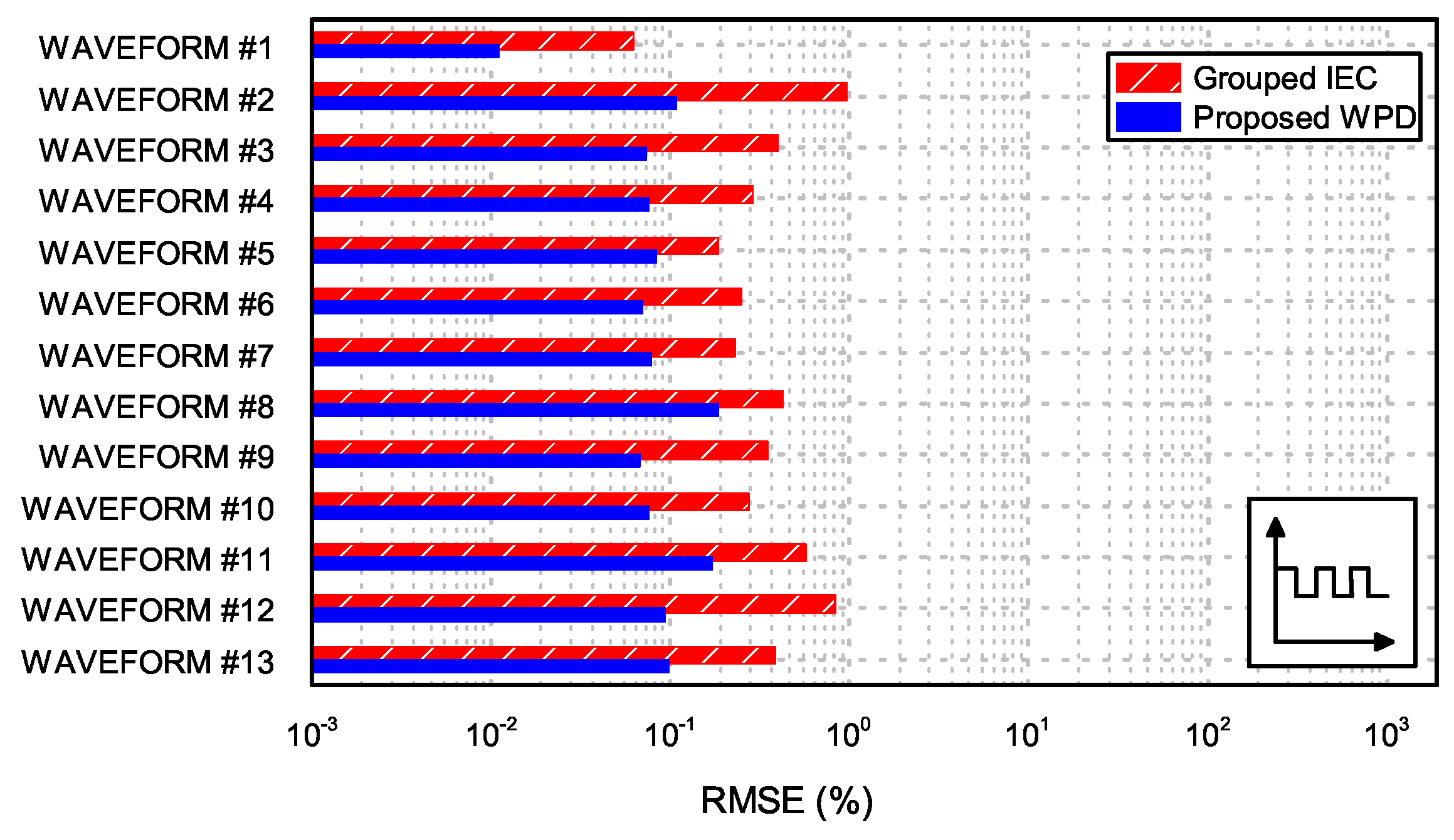
4.2. Validation for Stationary Conditions

In this section, an extensive analysis is presented for the case of Waveform 1, in steady state conditions. Figure 3 shows the obtained results for Waveform 1, along with the calculated errors.

The harmonic content was significantly more complex than single frequency signals, and it is possible to see that the results of the FFT slightly deviated from the expected values. The same happened with the grouped FFT and the proposed WPD method. In all of the cases, however, the errors were very low, always lower than 0.2%. Depending on the harmonic order and on the frequency content, the WPD errors were higher or lower than FFT. The bottom graph of Figure 3 shows a plot of the difference between the error of the WPD results and the error of the results of the grouped FFT (which resulted in being more accurate than standard FFT). This value indicated how worse WPD was performing with respect to the grouped FFT. Negative values mean that WPD was performing better. It is possible to see from Figure 3 that the error of the proposed WPD method was always lower than the IEC method, except for the orders four and 39 where, however, the difference was negligible (less than 0.005%). In any case, all the errors presented were extremely low, and all the methods were perfectly suitable for stationary harmonics.

The other 12 waveforms were assayed with the same methodology, and a summary of the obtained results is presented. Figure 4 shows that, among all the assayed waveforms, the maximum difference between the errors of the two methods was less than 0.35%, which represented the worst case. This means that in the case of stationary signals, the presented method was almost never worse than the FFT or the grouped FFT, and when it was, the deviation was negligible.

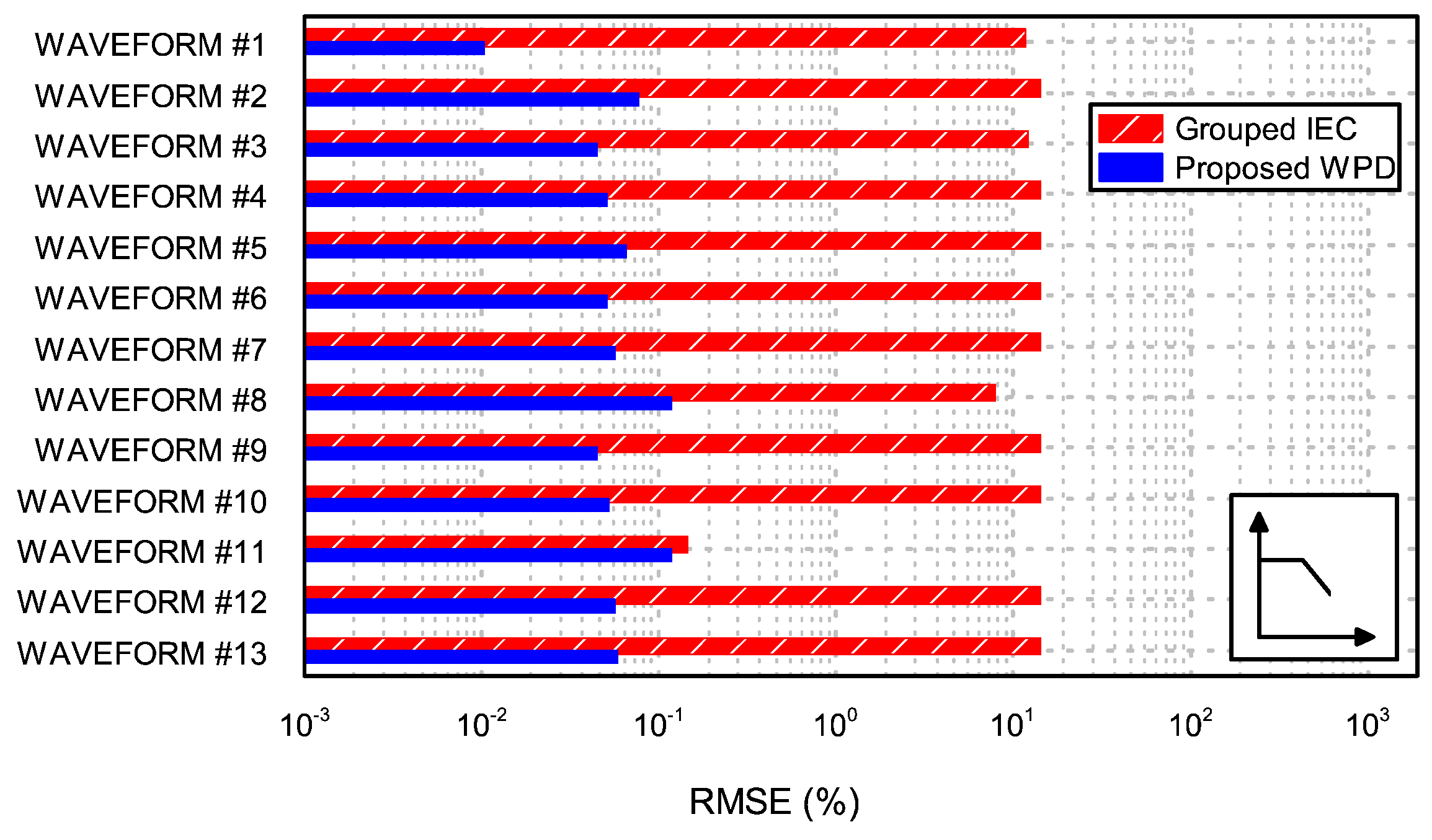
4.3. Validation for Non-Stationary Conditions

In this section, the performance of the proposed method in the case of non-stationary realistic waveforms is assessed. The results were compared to the strategy proposed by IEC 61000-4-7, i.e., grouped FFT. Among the scenarios discussed so far, this was the most relevant one, since it was the closest to reality, where voltage and current waveforms are often, if not always, non-stationary. As stated in Section 4.1, three different fluctuation patterns were applied to the 13 waveforms previously identified. In this regard, Figure 5 illustrates the three types of modulations that were used.

Figure 6 shows the results obtained for Waveform 1 with constant modulation. It can be easily seen how the proposed WPD method was significantly more accurate than the grouped FFT, which produced large errors. When the measured RMS content was less than 1%, the percentage of error was calculated with respect to the nominal voltage, according to the IEC 61000-4-7 standard [5]. The results of the conventional FFT produced even larger errors and, for the sake of clarity, are not presented. Depending on the harmonic order, the deviation of the proposed WPD method from the real content of the signal could vary, but it was always more accurate than the grouped IEC method. This is confirmed by the bottom graph of Figure 6, which shows the difference between the errors made by the two methods. As can be seen, all the values were negative, meaning that WPD always gave more accurate results than grouped FFT, and in some cases with a large difference. It can also be seen that, in both methods, the largest errors were usually produced when no harmonic content was expected. In this case, the appearance of non-zero values was due to the so-called energy leakage, i.e., part of the harmonic content of nearby bands leaked to a band where no content should be present. This affected both methods, but it was evident that WPD was significantly superior in dealing with this issue, providing a far better overall accuracy.

The other 12 waveforms were assayed with the same methodology, and a summary of the obtained results is presented. In this case, to quantify and compare the overall accuracy of the two methods, the Root Mean Squared Error (RMSE) can be employed:

$$RMSE=\sqrt{\frac{{\sum }_{h=1}^N{\epsilon }_{\mathrm{h}}^2}{N}}$$

(5)

where ${\epsilon }_{\mathrm{h}}$ is the error produced for order h, and N is the total number of bands, 50 in this case. This quantity is typically used in statistics to measure how well a distribution fits experimental data. However, in this case, it was used to aggregate the errors of each tested method over all harmonic orders into a single measure and have an estimation of the overall accuracy. The higher the RMSE, the lower the overall accuracy. Figure 7 shows the RMSE obtained with both methods, for all the considered waveforms (see Table 2). The constant modulation was employed (the same proposed by IEC 61000-4-7 for fluctuating harmonics). In order to better appreciate the large differences, results are plotted in logarithmic scale. The significantly lower RMSE for the proposed WPD method means a higher overall accuracy of the proposed method. Figure 8 and Figure 9 present the same analysis, but using the linear modulation and the flicker-type modulation, respectively.

It can be seen that the overall accuracy of the WPD method was always significantly superior to the grouped FFT, for all the tested waveforms and types of modulations. The only case where the overall accuracy of WPD was comparable with the grouped FFT was the case of Waveform 11 (square wave) with the linear modulation. However, even in this extremely non-realistic case, WPD showed a better performance.

Table A1. Maximum errors obtained for each validation assay.

	Stationary			Constant			Linear			Rectangular
ID	${\mathit{\epsilon }}_{\mathbf{max}}$ (%)	Order		${\mathit{\epsilon }}_{\mathbf{max}}$ (%)	Order		${\mathit{\epsilon }}_{\mathbf{max}}$ (%)	Order		${\mathit{\epsilon }}_{\mathbf{max}}$ (%)	Order
1	0.048	2		0.079	1		0.041	2		0.048	2
2	0.416	5		0.504	5		0.281	3		0.486	5
3	0.416	5		0.514	5		0.271	5		0.479	5
4	0.374	5		0.458	5		0.232	5		0.428	5
5	0.322	4		0.372	5		0.285	4		0.327	4
6	0.319	5		0.390	5		0.184	4		0.341	5
7	0.348	5		0.428	5		0.213	4		0.394	5
8	0.589	7		0.625	7		0.446	7		0.678 *	5
9	0.363	5		0.443	5		0.221	5		0.406	5
10	0.366	5		0.449	5		0.225	5		0.418	5
11	0.566	7		0.667	5		0.437	2		0.671	5
12	0.401	5		0.488	5		0.258	5		0.462	5
13	0.397	5		0.484	5		0.254	5		0.476	5

, reported in Appendix A, provides a summary of the maximum errors obtained in the calculation of individual harmonic components, for all the assayed waveforms, in the four validation scenarios (stationary and fluctuating). It can be seen that the maximum error never exceeded 1%, with the maximum obtained error being 0.678%. Although this was far from being a mathematical formulation of the error, it could be considered as an indication of the accuracy of the proposed method.

4.4. Computational Effort

A drawback of the proposed WPD method could be the high number of operations that must be performed. At each level of decomposition, the number of filtering operation increased exponentially, although the decimation allowed reducing the number of samples that were convolved with the filter coefficients. In order to characterize the computational effort required, a comparison was performed by analyzing the same waveform, under the same conditions, with both methods. Although it did not represent an exhaustive study of the computational complexity, a comparison of the time required by the two methods on the same computer, for the same signal, and under the same operating conditions can be considered as an indication of the relationship between the computational effort of the two methods. The same analysis was repeated 1000 times for each of the 13 waveforms described in Section 4.1, and later, the 13,000 results were averaged. The results, obtained on a $3.00$ $\mathrm{G}$$\mathrm{Hz}$ Intel Core i5-7400 CPU with 16 $\mathrm{MB}$ RAM computer, are reported in

Table 3. Comparison of the average computational time for both methods on the same computer.

Computational Time (FFT) (s)	Computational Time (WPD) (s)	Ratio WPD/FFT
3.6 × 10−4	5.2 × 10−2	148

.

As can be seen, the time required by the proposed WPD algorithm resulted in being, on average, 148-times higher than FFT. However, it can be seen that, at least on the testing machine, the method had the capability of being performed online, since the time required for the calculation was less than the duration of the analyzed signal, i.e., 10 cycles of the power frequency (approximately 200 $\mathrm{m}$$\mathrm{s}$). A possible strategy to reduce the computation time is to implement the proposed method on an Field Programmable Gate Array (FPGA) since the structure, based on the iterative application of the same filter, is particularly suitable for hardware implementation and the time reduction could be significant, as demonstrated by recent works [23,30].

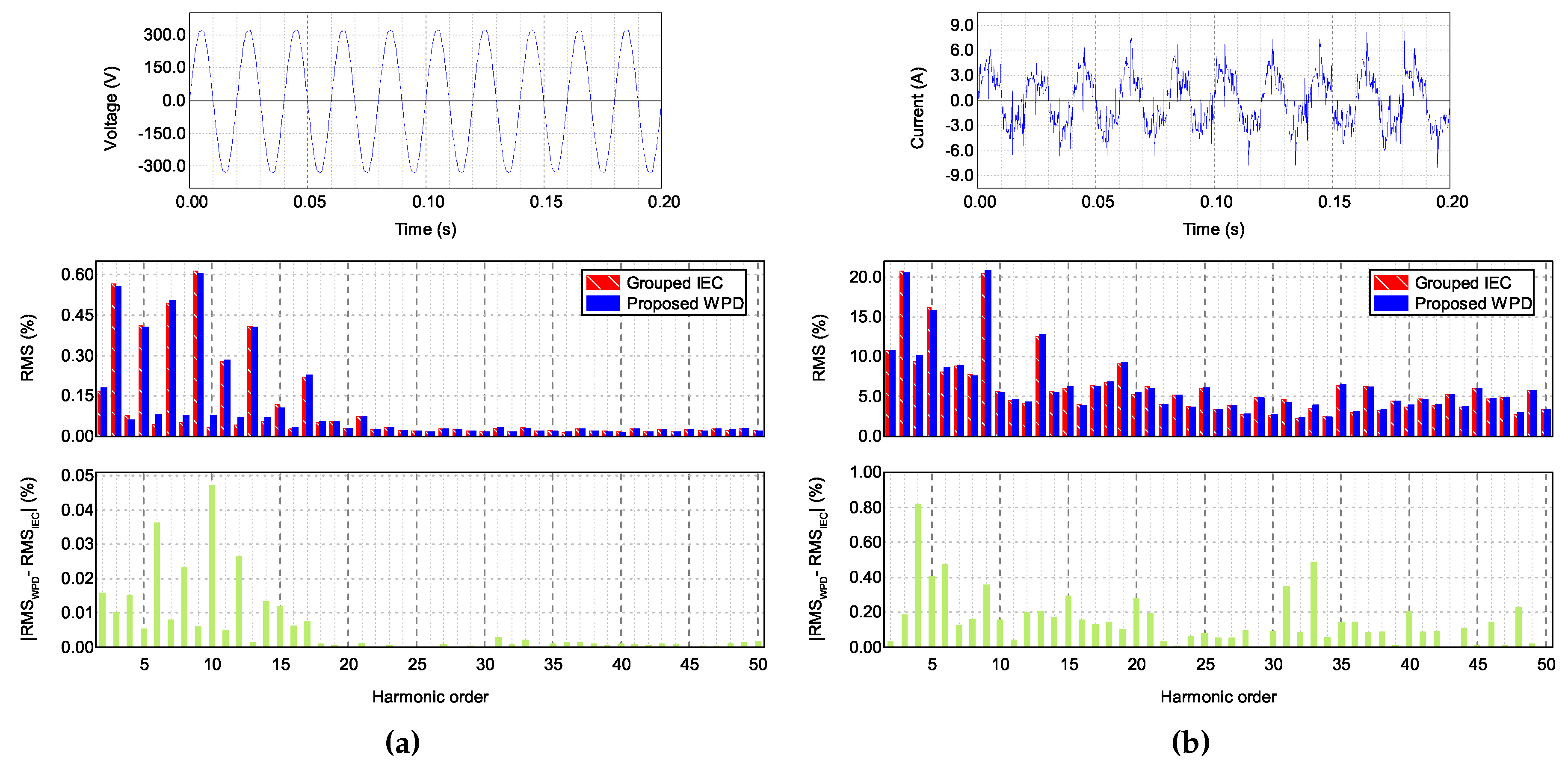
5. Analysis of Real Signals

The newly proposed method, after being validated, was employed to analyze real waveforms. In order to obtain real waveforms, measurements were taken at the point of connection of an Active Front End (AFD) device. It as a three leg 50 $\mathrm{k}$$\mathrm{W}$ converter, with a 20 $\mathrm{k}$$\mathrm{Hz}$ switching frequency. Current and voltage waveforms were acquired using a NI PXIe-6124 module (installed on an NI PXIe-1071 chassis), equipped with a Pico TA044 70 $\mathrm{M}$$\mathrm{Hz}$ 7000 $\mathrm{V}$ differential voltage probe and a Tektronix TCP2020 50 $\mathrm{M}$$\mathrm{Hz}$ 20 $\mathrm{A}$ AC/DC current probe. The assayed AFD was designed to obtain low power losses, high efficiency (>96%), and most importantly, to produce low harmonic distortion. At nominal power, the THD was less than 0.6%. Therefore, in order to obtain signals with higher harmonic content, the harmonic distortion was enhanced by operating the device at 5% of its nominal power. In this way, the fundamental current was greatly reduced, while the harmonic components were only slightly reduced, increasing the current THD up to 50%.

The top graphs of Figure 10a,b show the acquired voltage and current waveforms, respectively, with a total duration of 10 cycles of the fundamental (approximately $0.2$ $\mathrm{s}$), according to the IEC 61000-4-7 standard. It must be noted that in these cases, the error could not be calculated since the real energy content of each harmonic group was not known a priori. For this reason, the bottom plots of Figure 10a,b show the absolute difference between the RMS values obtained with the two methods, for each harmonic group, and not the error. Hence, it is not possible to know which method performed better, but only how different the results could be from each other. The voltage waveform in Figure 10a offers the possibility to analyze a mostly stationary signal. It can be observed that, in this case, the results obtained with the proposed WPD method were very similar to those obtained with the IEC method, and the differences between RMS values were close to zero for all harmonic orders. On the other hand, the current waveform in Figure 10b has a visible fluctuating character, offering the possibility to test the proposed WPD method with a real non-stationary signal. In this case, the differences between the two methods were higher, up to almost 1%. These results confirmed the conclusions of Section 4, i.e., that the WPD method was equally valid as the IEC Fourier strategy for analyzing stationary signals, but that differences arise under fluctuating conditions, where FFT is known to be inaccurate.

6. Conclusions

This paper presented the validation and characterization of a wavelet based method for the accurate assessment of harmonic content in power systems under stationary and non-stationary conditions, using a WPD algorithm. Although other methods have been proposed in the last few years, some of them even using wavelets, Fourier analysis is still the preferred choice for power quality analyzers and the recommended approach according to IEC standards. It is however evident that Fourier analysis is inadequate for assessing harmonic content under non-stationary conditions, which is the most common situation in power systems. Even IEC 61000-4-7 recognizes this limitation, proposing a grouping strategy for adapting FFT to fluctuating harmonics. The IEC grouping strategy, however, can produce large errors in the case of fluctuating signals, as shown in this paper. The proposed method was therefore compared not only to standard FFT, but also to the IEC grouped FFT method, showing its superior performance with respect to both. After verifying compliance with the IEC precision requirements and validating the method using simulated waveforms with real harmonic content, the method was employed to measure real voltage and current signals. This produced results similar to those obtained in the validation. The reliability of the method was clearly proven, and its performance was superior under fluctuating conditions. On the one hand, researchers are more and more transitioning to more reliable tools, while on the other hand, no methods have been shown to be able to comply with IEC standards and at the same time be precise enough to measure fluctuating harmonics. This paper intended to fill the gap between the research community and the application in the field, illustrating and validating a method whose performance was largely superior to the grouped FFT in assessing fluctuating harmonics. Moreover, the proposed method was shown to perform better than grouped FFT even under stationary conditions, and in the few cases when it did not perform better, the error was always within the IEC accuracy limits for steady-state signals. Lastly, the proposed frequency bands, time window, and bandwidth were, for the first time, compliant with the IEC 61000-4-7 and IEC 61000-4-30 requirements. This was achieved by an accurate selection of the decomposition tree and filter characteristics. The features of the proposed method made it suitable for implementation in Class I Power Quality analyzers, allowing a highly accurate estimation of harmonic content in power systems, both in stationary and non-stationary conditions.

References

1. Kalair, A.; Abas, N.; Kalair, A.R.; Saleem, Z.; Khan, N. Review of harmonic analysis, modeling and mitigation techniques. Renew. Sustain. Energy Rev. 2017, 78, 1152–1187. [Google Scholar] [CrossRef]
2. Sharma, H.; Rylander, M.; Dorr, D. Grid impacts due to increased penetration of newer harmonic sources. IEEE Trans. Ind. Appl. 2016, 52, 99–104. [Google Scholar] [CrossRef]
3. Liang, X. Emerging Power Quality Challenges Due to Integration of Renewable Energy Sources. IEEE Trans. Ind. Appl. 2017, 53, 855–866. [Google Scholar] [CrossRef]
4. Moeed Amjad, A.; Salam, Z. A review of soft computing methods for harmonics elimination PWM for inverters in renewable energy conversion systems. Renew. Sustain. Energy Rev. 2014, 33, 141–153. [Google Scholar] [CrossRef]
5. Electromagnetic Compatibility (EMC)—Part 4-7: Testing and Measurement Techniques—General Guide on Harmonics and Interharmonics Measurements and Instrumentation, for Power Supply Systems and Equipment Connected Thereto. IEC 61000-4-7:2002+AMD1:2008.
6. IEEE Recommended Practices and Requirements for Harmonic Control in Electrical Power Systems. In IEEE Std. 519-2014; IEEE, 2014.
7. Clarkson, P.; Wright, P.S. A wavelet based method of measuring fluctuating harmonics for determining the filter time constant of IEC standard harmonic analyzers. IEEE Trans. Instrum. Meas. 2005, 54, 488–491. [Google Scholar] [CrossRef]
8. Jain, S.K.; Singh, S.N. Harmonics estimation in emerging power system: Key issues and challenges. Electr. Power Syst. Res. 2011, 81, 1754–1766. [Google Scholar] [CrossRef]
9. Mostarac, P.; Malarić, R.; Mostarac, K.; Jurčević, M. Noise reduction of power quality measurements with time-frequency depth analysis. Energies 2019, 12, 1052. [Google Scholar] [CrossRef]
10. Wang, C.; Yang, R.; Yu, Q. Wavelet transform based energy management strategies for plug-in hybrid electric vehicles considering temperature uncertainty. Appl. Energy 2019, 256, 113928. [Google Scholar] [CrossRef]
11. Telesca, L.; Guignard, F.; Helbig, N.; Kanevski, M. Wavelet Scale Variance Analysis of Wind Extremes in Mountainous Terrains. Energies 2019, 12, 3048. [Google Scholar] [CrossRef]
12. Zhu, H.; Li, X.; Sun, Q.; Nie, L.; Yao, J.; Zhao, G. A power prediction method for photovoltaic power plant based on wavelet decomposition and artificial neural networks. Energies 2016, 9, 11. [Google Scholar] [CrossRef]
13. Avdakovic, S.; Lukac, A.; Nuhanovic, A.; Music, M. Wind speed data analysis using wavelet transform. World Acad. Sci. Eng. Technol. 2011, 51, 829–833. [Google Scholar]
14. Karmacharya, I.M.; Gokaraju, R. Fault Location in Ungrounded Photovoltaic System Using Wavelets and ANN. IEEE Trans. Power Deliv. 2018, 33, 549–559. [Google Scholar] [CrossRef]
15. Yoon, W.K.; Devaney, M.J. Reactive power measurement using the wavelet transform. IEEE Trans. Instrum. Meas. 2000, 49, 246–252. [Google Scholar] [CrossRef]
16. Morsi, W.G.; El-Hawary, M.E. On the application of wavelet transform for symmetrical components computations in the presence of stationary and non-stationary power quality disturbances. Electr. Power Syst. Res. 2011, 81, 1373–1380. [Google Scholar] [CrossRef]
17. Deokar, S.A.; Waghmare, L.M. Integrated DWT-FFT approach for detection and classification of power quality disturbances. Int. J. Electr. Power Energy Syst. 2014, 61, 594–605. [Google Scholar] [CrossRef]
18. De Apráiz, M.; Barros, J.; Diego, R.I. A real-time method for time-frequency detection of transient disturbances in voltage supply systems. Electr. Power Syst. Res. 2014, 108, 103–112. [Google Scholar] [CrossRef]
19. Latran, M.B.; Teke, A. A novel wavelet transform based voltage sag/swell detection algorithm. Int. J. Electr. Power Energy Syst. 2015, 71, 131–139. [Google Scholar] [CrossRef]
20. Alves, D.K.; Costa, F.B.; de Araujo Ribeiro, R.L.; de Sousa Neto, C.M.; de Oliveira, T. Power Measurement Using the Maximal Overlap Discrete Wavelet Transform. IEEE Trans. Ind. Electron. 2017, 64, 3177–3187. [Google Scholar] [CrossRef]
21. Hamid, E.Y.; Yokoyama, N.; Kawasaki, Z.I. Rms and Power Measurements: A Wavelet Packet Transform Approach. IEEJ Trans. Power Energy 2002, 122, 599–606. [Google Scholar] [CrossRef]
22. Eren, L.; Unal, M.; Devaney, M.J. Harmonic Analysis Via Wavelet Packet Decomposition Using Special Elliptic Half-Band Filters. IEEE Trans. Instrum. Meas. 2007, 56, 2289–2293. [Google Scholar] [CrossRef]
23. Tiwari, V.K.; Umarikar, A.C.; Jain, T. Fast Amplitude Estimation of Harmonics Using Undecimated Wavelet Packet Transform and Its Hardware Implementation. IEEE Trans. Instrum. Meas. 2017, 1–13. [Google Scholar] [CrossRef]
24. Diego, R.I.; Barros, J. Global Method for Time-Frequency Analysis of Harmonic Distortion in Power Systems Using the Wavelet Packet Transform. Electr. Power Syst. Res. 2009, 79, 1226–1239. [Google Scholar] [CrossRef]
25. Barros, J.; Diego, R.I. Analysis of Harmonics in Power Systems Using the Wavelet Packet Transform. IEEE Trans. Instrum. Meas. 2008, 57, 63–69. [Google Scholar] [CrossRef]
26. Bruna, J.; Melero, J.J. Selection of the Most Suitable Decomposition Filter for the Measurement of Fluctuating Harmonics. IEEE Trans. Instrum. Meas. 2016, 65, 2587–2594. [Google Scholar] [CrossRef]
27. Mallat, S.G. A Wavelet Tour of Signal Processing, 2nd ed.; Academic Press: Cambridge, MA, USA, 1999. [Google Scholar]
28. NPL. Power Quality Waveform Library. Available online: http://resource.npl.co.uk/waveform/ (accessed on 30 October 2019).
29. Brekke, K.; Seljeseth, H.; Mogstad, O. Rapid Voltage Changes—Definition and Minimum Requirements. In Proceedings of the 20th International Conference on Electricity Distribution (CIRED), Prague, Czech Republic, 8–11 June 2009. [Google Scholar] [CrossRef]
30. Tiwari, V.K.; Jain, S.K. Hardware Implementation of Polyphase-Decomposition-Based Wavelet Filters for Power System Harmonics Estimation. IEEE Trans. Instrum. Meas. 2016, 65, 1585–1595. [Google Scholar] [CrossRef]
Figure 1. Wavelet Packet Decomposition (WPD) filtering and decimation scheme.
Energies 12 04389 g001
Figure 2. Top: errors of the proposed method with steady-state single frequency signals. Bottom: comparison of the error produced by the conventional FFT, the grouped IEC, and the WPD methods in case of single frequency signals, under fluctuating conditions (as explained in the text). The grey lines show the limits provided by IEC 61000-4-7 for stationary conditions.
Energies 12 04389 g002
Figure 3. Analysis of the IEC 61000-3-2 limits waveform under stationary conditions. The comparison is made between the IEC, the grouped IEC, and the proposed WPD methods. The upper graph shows the spectrum of the RMS content of each IEC frequency band for the three methods, compared to the real content. The middle graph shows the errors for each frequency band. The difference between the errors is shown in the bottom graph.
Energies 12 04389 g003
Figure 4. Maximum positive difference between the error of the WPD and grouped IEC methods.
Energies 12 04389 g004
Figure 5. Schematic illustration of the employed modulation patterns. From left to right: constant modulation, linear modulation, and flicker-type modulation.
Energies 12 04389 g005
Figure 6. Analysis of the IEC 61000-3-2 limits waveform under non-stationary conditions (constant modulation). The upper graph shows the spectrum of the RMS content of each IEC frequency band for the three methods, compared to the real content. The middle graph shows the errors for each frequency band. The difference between the errors is shown in the bottom graph.
Energies 12 04389 g006
Figure 7. RMSE for each assessed waveform under fluctuating conditions, for grouped IEC and WPD, in the case of constant modulation.
Energies 12 04389 g007
Figure 8. RMSE for each assessed waveform under fluctuating conditions, for grouped IEC and WPD, in the case of linear modulation (motor-start type).
Energies 12 04389 g008
Figure 9. RMSE for each assessed waveform under fluctuating conditions, for grouped IEC and WPD, in the case of flicker-type rectangular modulation.
Energies 12 04389 g009
Figure 10. Analysis of real waveforms with a stationary (a) and non-stationary (b) character. The top graphs show the waveforms in the time domain, the middle graphs the harmonic content, and the bottom graphs the absolute difference between the proposed method and the IEC strategy.
Energies 12 04389 g010