Article

Looking for Energy Losses of a Rotary Permanent Magnet Magnetic Refrigerator to Optimize Its Performances

by
Angelo Maiorino
1,*,
Antongiulio Mauro
1,
Manuel Gesù Del Duca
1,
Adrián Mota-Babiloni
2 and
Ciro Aprea
1
1
Department of Industrial Engineering, Università di Salerno, Via Giovanni Paolo II, 132, Fisciano, 84084 Salerno, Italy
2
ISTENER Research Group, Department of Mechanical Engineering and Construction, Campus de Riu Sec s/n, Universitat Jaume I, E-12071 Castelló de la Plana, Spain
*
Author to whom correspondence should be addressed.
Energies 2019, 12(22), 4388; https://doi.org/10.3390/en12224388
Submission received: 27 September 2019 / Revised: 22 October 2019 / Accepted: 14 November 2019 / Published: 19 November 2019
(This article belongs to the Special Issue Refrigeration Systems and Applications 2019)

Abstract

:
In this paper, an extensive study on the energy losses of a magnetic refrigerator prototype developed at University of Salerno, named ‘8MAG’, is carried out with the aim to improve the performance of such a system. The design details of ‘8MAG’ evidences both mechanical and thermal losses, which are mainly attributed to the eddy currents generation into the support of the regenerators (magnetocaloric wheel) and the parasitic heat load of the rotary valve. The latter component is fundamental since it imparts the direction of the heat transfer fluid distribution through the regenerators and it serves as a drive shaft for the magnetic assembly. The energy losses concerning eddy currents and parasitic heat load are evaluated by two uncoupled models, which are validated by experimental data obtained with different operating conditions. Then, the achievable coefficient of performance (COP) improvements of ‘8MAG’ are estimated, showing that reducing eddy currents generation (by changing the material of the magnetocaloric wheel) and the parasitic heat load (enhancing the insulation of the rotary valve) can lead to increase the COP from 2.5 to 2.8 (+12.0%) and 3.0 (+20%), respectively, and to 3.3 (+32%), combining both improvements, with an hot source temperature of 22 °C and 2 K of temperature span.

1. Introduction

Magnetic refrigeration is an emerging and environmental-friendly technology that uses a solid refrigerant exploiting the magneto-caloric effect (MCE), which is represented by a temperature change of the material when it is subjected to a change of an external magnetic field. Studies showed that this technology could lead to 20–30% energy savings compared to vapor compression refrigeration because of magnetization work recovery and lower entropy generation [1,2,3,4], as well as a reduction of the environmental impact of the refrigeration system [5,6]. Several prototypes have been designed and built so far, and their performances strictly depend both on the system design and operating conditions, as well as on the employed magnetocaloric material [7]. Although magnetic refrigeration is a promising technology to substitute vapor-compression systems, its performances are still lower than those provided by vapor-compression systems, regarding cooling power, temperature span, efficiency, and system design. Several apparatus, based on different constructive concepts, have been presented and widely characterized in the literature over the years [8,9,10,11,12,13,14,15,16,17,18,19,20]. A comprehensive overview of these experimental devices built so far can be found in different recent reviews [7,21].
Energy efficiency is one of the crucial characteristics to allow this technology becoming mature for markets, as well as to compare different system concepts. Several strategies to improve energy efficiency have been explored, whether focusing on theoretical aspects and thermodynamic cycles [22,23,24] or performing extensive studies on system energy performances [10,25,26,27], as well as coupling magnetic refrigerators with systems such as Stirling motors, geothermal probes, and ejectors [28,29,30,31]. Furthermore, different studies have been conducted on the optimal control of magnetic cooling devices to improve their performance, using both an experimental [32] and a modelling approach [33,34].
A rotary permanent magnet magnetic refrigerator, named ‘8MAG’, was developed at University of Salerno [35] and first experimental data were carried out [15,16] concerning cooling power, temperature span and coefficient of performance (COP). The optimization of existing prototypes, in terms of design and performance, is currently a common subject in the magnetic refrigeration literature [36,37,38,39,40,41], showing COPs of the order of 5 with 5 K of temperature span and 0.5 with 25 K of temperature span. ‘8MAG’ showed a maximum COP of 2.5 with 2 K of temperature span and an hot source temperature (TH) equal to 22 °C [35]. Furthermore, ‘8MAG’ showed a maximum second-law efficiency of 2.4% at TH = 22 °C and a temperature span of 3.3 K. These results are comparable to the performance of the magnetic refrigerator prototype presented by Capovilla et al. [42].
Then, in the present work, several numerical analyses have been performed to estimate parasitic losses of ‘8MAG’ and to identify a way for improving prototype performances. In detail, eddy currents generation and the parasitic thermal load were addressed. Identifying the possible energy losses can help to highlight the improvements which are needed to be made to a magnetic refrigerator in different operating conditions. Nevertheless, a detailed study is mandatory to characterize these energy losses and analyse their effect on energy performance. Some losses can be easily identified and quantified by a few experimental tests, such as friction losses, but others are more difficult to characterize, with several experiments required. Hence, to reduce the experimental efforts and generalize the results, the characterization of this kind of energy losses was performed by mathematical models, properly defined and validated.

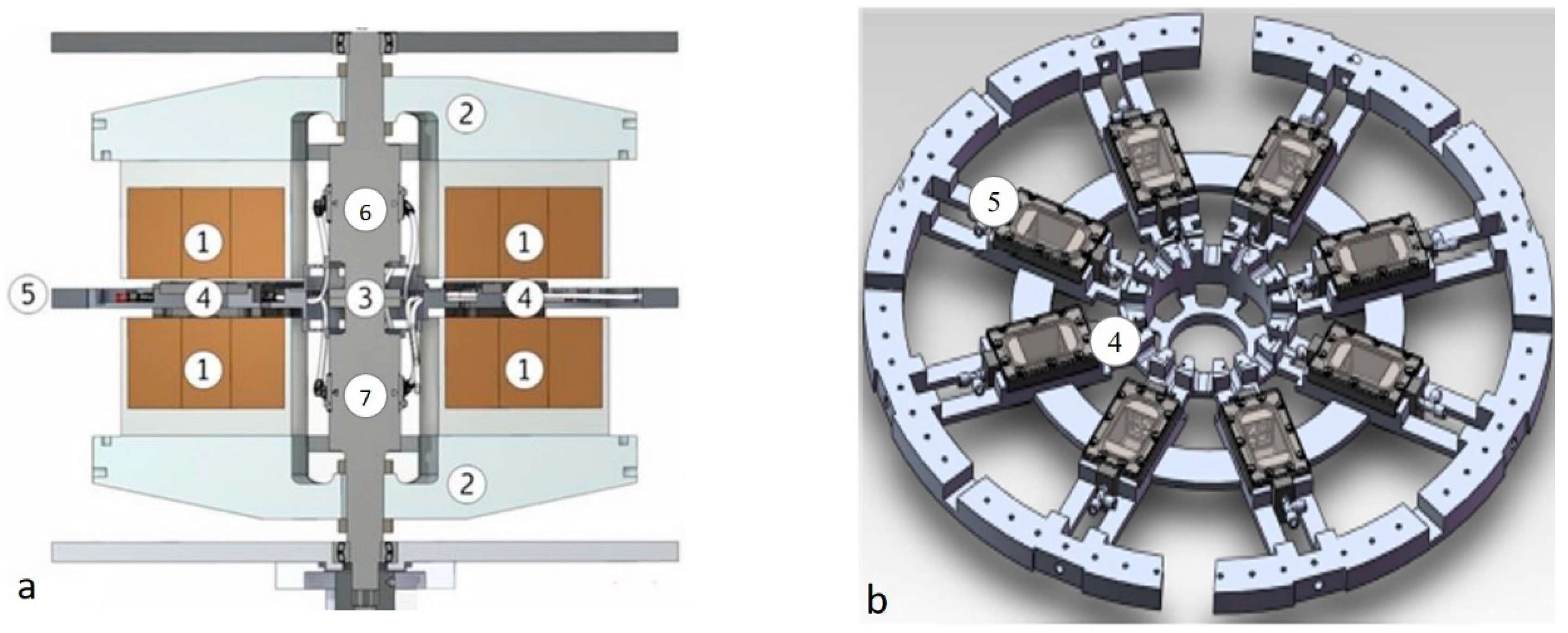
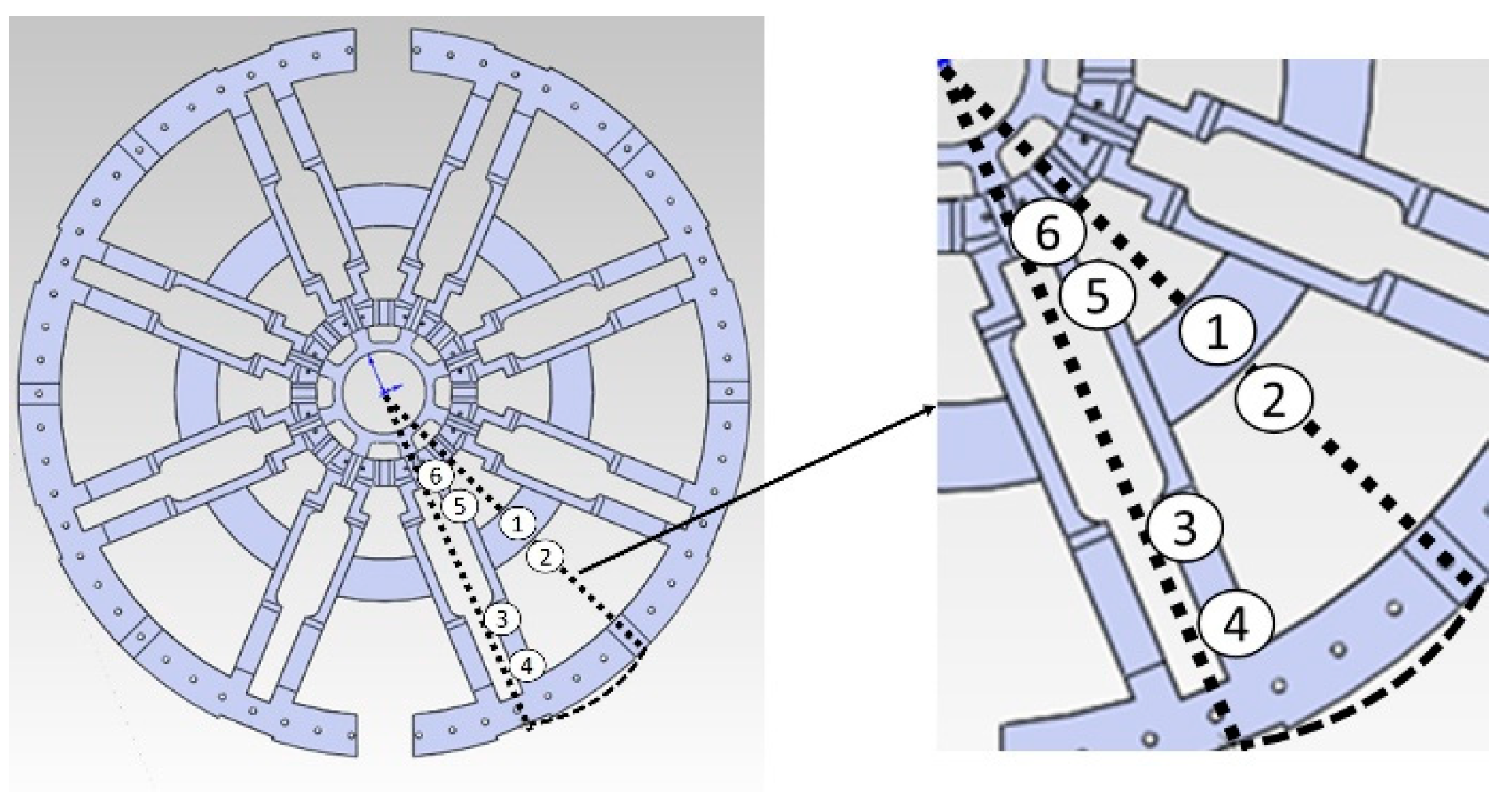
2. The Prototype and the Experimental Measurement System

A detailed description of the experimental apparatus (‘8MAG’) was already provided in Aprea et al. [16]. However, it is needed to focus on some design details to identify the most relevant energy losses. ‘8MAG’ is a rotative permanent magnet prototype equipped with two magnets disposed at 180 degree based on a double U configuration with about 1.2 T. Eight static regenerators, located in the air gap (43 mm) between poles of magnets and disposed in 45 degrees among them, are alternatively magnetized and demagnetized with the rotation of the magnets assembly. The regenerators are fixed on a frame, named magnetocaloric wheel (MCW), which is located inside the magnets gap and made of a diamagnetic aluminium alloy.
A rotary valve, coaxial with the magnetic assembly, imparts the direction of the heat transfer fluid (demineralized water) distribution through the regenerators. The rotary valve consists of two main parts: a stator (fixed to the MCW) and a rotor (connected to the drive shaft). The rotor acts as a rotary manifold and as a shaft for the magnetic system. The stator is divided into a hot sub-valve and a cold sub-valve and each sub-valve allows the connection between the regenerators and the rotary manifold. Each part of the rotary valve is made in stainless steel.
The prototype is shown in Figure 1 and it was widely described in Aprea et al. [16].
Several sensors were used to measure the most important variables to characterize the energy performance of the magnetic refrigerator prototype.
A torque meter has been used to measure mechanical torque, an encoder provides angular speed, calibrated resistance temperature detectors (RTD) four wires have been used for temperature measurements. Torque and temperature measurements have been carried out using a national instruments (NI) compactDAQ system and the NI LabVIEW software. Axial mechanical power has been measured using the torque meter and controlling the angular speed of a direct current (DC) brushless motor in closed loop through. The test apparatus is equipped with a 32-bit analog to digital (A/D) converter acquisition cards with sampling rate up to 10 kHz. In Table 1, a summary of the used instrumentation and relative accuracy are reported.

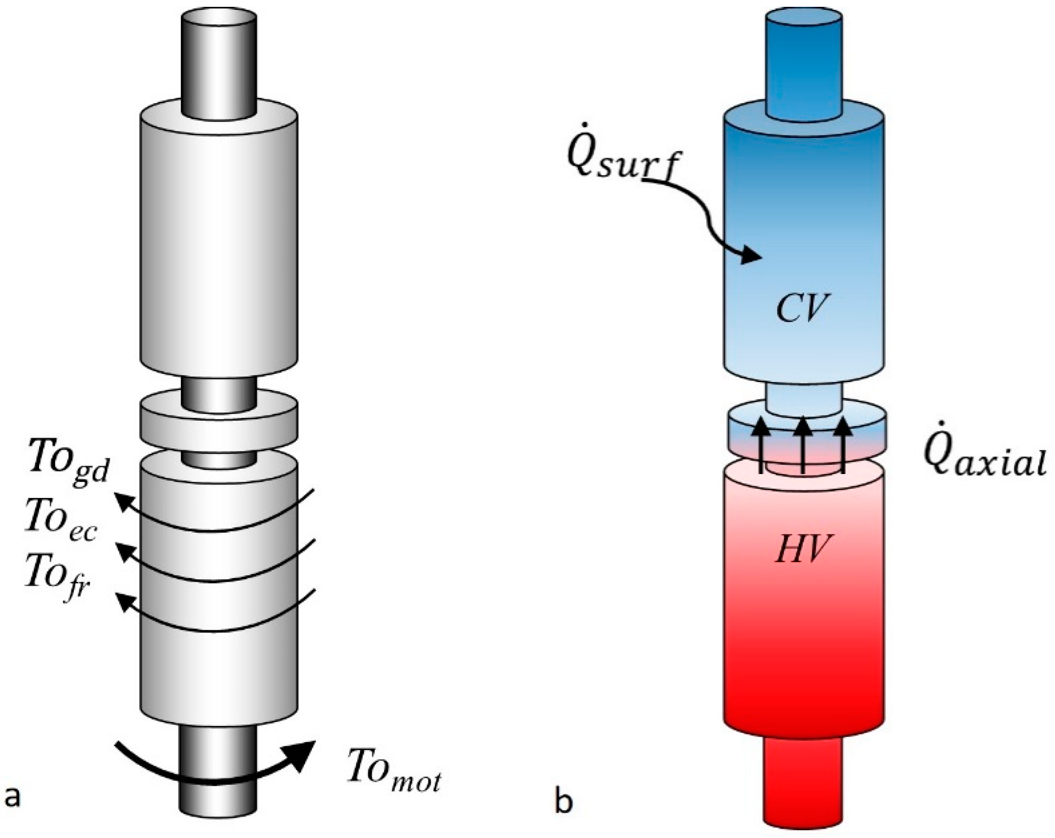
3. Energy Losses Model

Considering the operating mode of ‘8MAG’ and its design details, two different energy losses can be identified: mechanical losses and thermal losses. A core part of the entire assembly is the rotary valve, and therefore the overall study about energy losses can be performed focusing only on this component. Indeed, the rotary valve serves both as a drive shaft and as a thermal driver, distributing the cooling capacity and heat to be rejected. Hence, the model of energy losses, developed in COMSOL environment, is divided into two sub-models: the mechanical model and the thermal model. Both are graphically represented in Figure 2.

3.1. Mechanical Model

The work needed to magnetize and demagnetize the regenerators depends on the rotation of the magnetic system by the rotary valve. Hence, a resistant torque (TOgd) acts on this component, with a magnitude dependent on the working temperatures of the regenerators (hot and cold end). In detail, the magnitude of the resistant torque follows an oscillating trend, according to the alternative attraction and rejection of the magnets during the AMR cycle. This oscillation reduces with the increase of the rotational frequency due to the inertial phenomena related to the distribution of the rotating mass of the magnets. However, other two energy losses must be considered in ‘8MAG’ related to the drive shaft, and therefore to the rotary valve.
The rotation of the magnetic system allows to magnetize and demagnetize the regenerators placed in the MCW. During the magnetization and demagnetization of the regenerators, also the MCW is subjected to the magnetic field, with the same intensity and frequency of the regenerators. This fact leads to generate eddy currents due to the electrical conductivity of aluminium. The occurrence of eddy currents causes a further resistant torque (TOec) that leads to increase the work needed to move the magnetic assembly. Moreover, the friction caused by the sliding of the bearings and seals of the rotary valve represents an additional resistant torque (TOfr) on the drive shaft. Observing Figure 2, it is possible to write the following torque balance equation at steady-state conditions (neglecting the inertial term)
T o t o t ( ω , T g d , β ) = T o g d ( T g d , β ) + T o e c ( ω , β ) + T o f r ( ω ) ,
where β is the angular position of the magnets, T g d is the working temperature of the regenerators, and ω is the rotational speed of the magnetic assembly, expressed in rotations per minute (rpm).
Then, the mechanical power balance, referred to a complete rotation, can be written as
W ˙ t o t ( ω , T ) = W ˙ g d ( ω , T ) + W ˙ e c ( ω ) + W ˙ f r ( ω ) ,
where W ˙ e c and W ˙ f r represent the additional mechanical power required as a result of the mechanical losses ( W ˙ l o s s ). These latter two terms are considered in this work since they are source of losses that could be recovered. In Equation (2), the eddy currents generation in the magnetocaloric material and the air friction were neglected.
The evaluation of the effect of eddy currents (ECL—eddy currents losses), and then, the calculation of TOec, was performed by a mathematical model composed by three sub-model: the static magnetic field model (SMF), the stationary eddy currents power dissipation model (SECP), and the stationary thermal model (ST). The friction term ( W ˙ f r ( ω ) ) was estimated by a semi-empirical approach, using technical data of the bearings and seals of the rotary valve and measuring the resistant torque ( T o f r ( ω ) ) to the rotary valve without the MCW and regenerators. Hence, it was possible to measure the resistant torque related to friction effects.

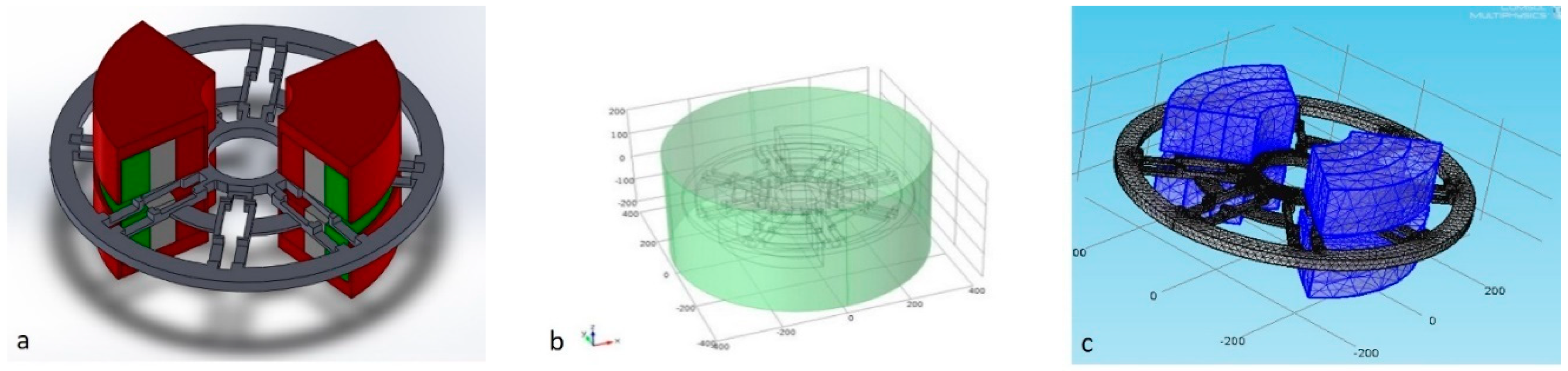
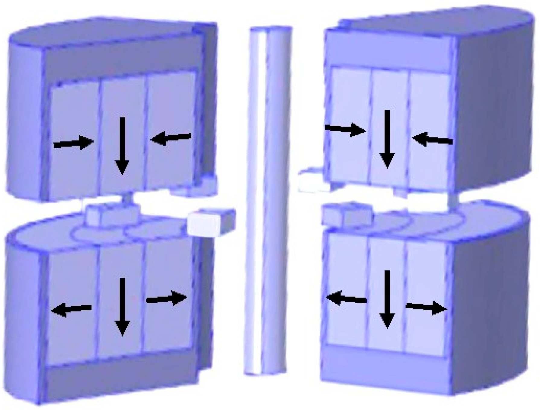
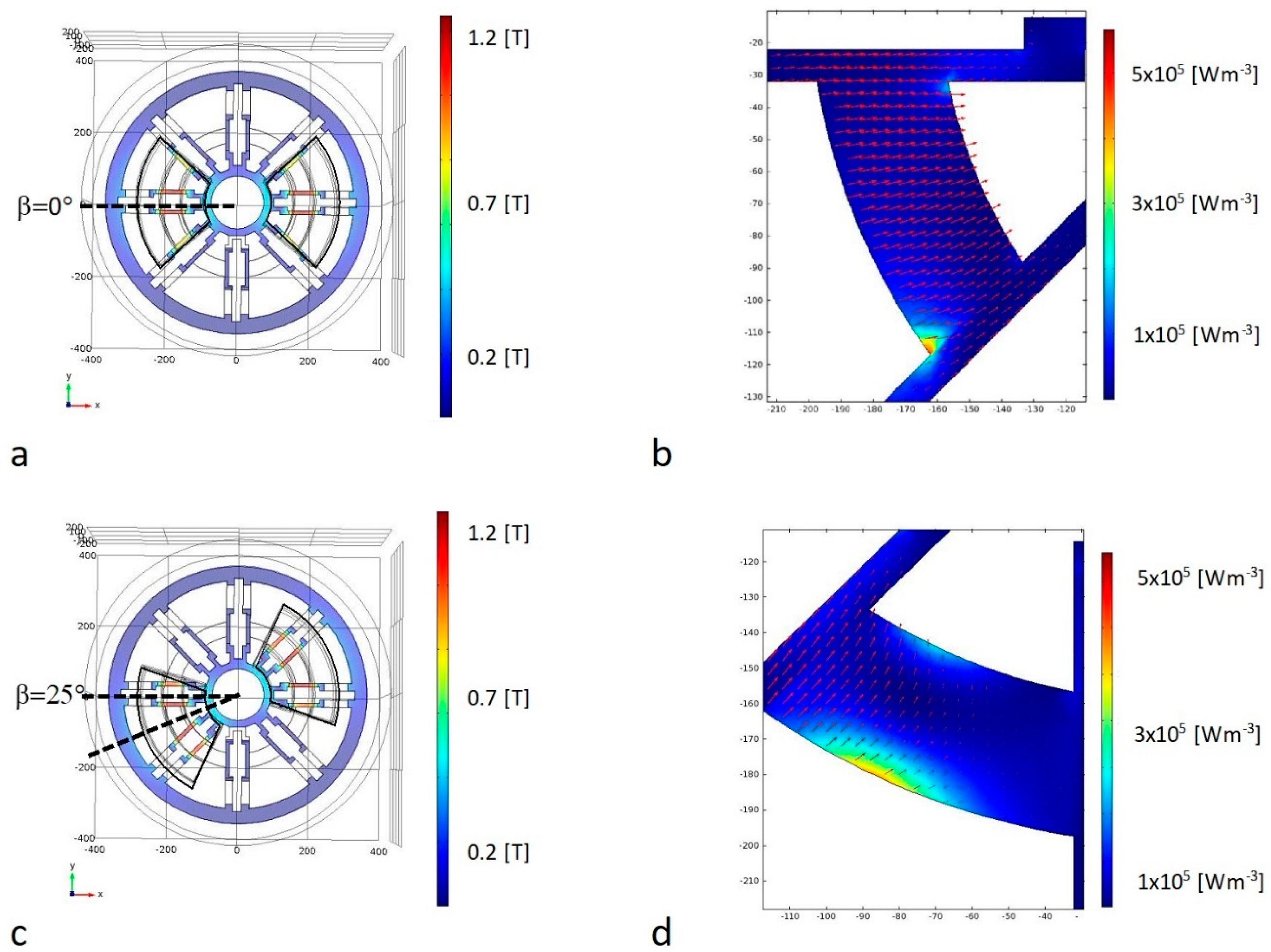
3.1.1. Static Magnetic Field Model

The evaluation of the magnetic field within the air gap, and therefore the intensity of the magnetic field to which the MCW is subjected, was carried out by a finite element method (FEM) analysis (see Figure 3). First, the domain under investigation was defined according to the real geometry of the magnetic assembly and the MCW. Then, a simplified geometry was designed to reduce computational time, neglecting holes, geometrical singularity, and low-relevant complex details. The entire geometry was included in a cylindrical volume with a diameter equal to 2.5 times of the diameter of the MCW and a height equal to 2.5 times of the height of the magnetic assembly. Three different meshes were tested: coarser (with 29,065 elements), normal (with 58,605 elements) and extremely fine (with 1,322,712 elements). A preliminary analysis of the standard deviation of the simulated magnetic flux density allowed to choose the best solution, which was the normal mesh with 58,605 elements.
The magnetic assembly was characterized considering the Halbach array configuration used in ‘8MAG’ (see Figure 4), where each segment is made of sintered NdFeB with a magnetic remanence (Br) of 1370 mT.
The model is defined by Maxwell’s equation
× H = J + D E t , × E = B t , ·   D E = ρ q , · B = 0 ,
where H is the magnetic field intensity (in A m−1), B is the magnetic flux density (T), E is the electric field intensity (V m−1), D E the electric flux density (C m−2), J is the electric current density (A m−2) and ρ q is the volume charge density (C m−3). The considered constitutive relations are shown in Equations (4)–(6)
D E = ε 0 E + P ,
B = μ 0 ( H + M ) ,
J = σ E ,
where ε 0 is the vacuum permittivity (in F m−1), P is the electric polarization (in C m−2), μ 0 is the vacuum permeability (in H m−1), M is the magnetization (in A m−1) and σ is the electrical conductivity. The boundary conditions at the material interfaces and physical boundaries are represented by the equations
n 2 × ( E 1 E 2 ) = 0 ,
n 2 × ( D E 1 D E 2 ) = ρ s ,
n 2 × ( H 1 H 2 ) = J s ,
n 2 × ( B 1 B 2 ) = 0 .
At last, considering the current continuity equation (Equation (11)), a further interface condition for the current density was introduced (Equation (12)).
· J = ρ q t ,
n 2 · ( J 1 J 2 ) = ρ s t .
In Equations (8) and (12), ρ s represents the surface charge density whereas, in Equation (9), J s represents the surface current density. The SMF sub-model provides, as output, the magnetic field intensity and the distribution of the magnetic field within the investigated domain.

3.1.2. Stationary Eddy Currents Power Dissipation Model

The results of the SMF sub-model (intensity of the magnetic field and its distribution) represent the input of the second sub-model, that is the SECP model, which aims to evaluate eddy currents generation inside the MCW.
To achieve this target, a Lorentz type induced current density term is included in the previous equation set (Equations (11) and (12)). Magnetic field rotation is simulated supposing that the magnets are rotating at a constant rotational speed ω. Different steady-state simulations were performed at various relative magnets/wheel positions (β) simulating a complete rotation of the magnets. The effect of magnetic field variation in the MCW, due to the presence of regenerators, has been neglected, thus regenerators have not been included in the modelling.
The Lorentz term is related to the rotational speed of the magnets, as
v = ω ( y , x , 0 ) .
Then, the eddy currents dissipation, in terms of resistive losses, can be calculated as
q e c ( x , y , z ) = σ J 2 ,
where σ is the electrical conductivity. The global power dissipated due to eddy currents is
Q e c = V σ J 2 .
where V is the geometrical volume defined by the mesh. Results show both the typical vortices formation of induced currents in the metal because of the longitudinal magnetic field gradient. Furthermore, due to the lack of axial symmetry of the MCW geometry, eddy current dissipation results to be a function of the relative rotation β. Figure 5 shows the magnetic flux density in the MCW (Figure 5a–c), the induced current generated (red arrow in Figure 5b–d) and the specific power generated in the aluminium (Figure 5b–d) for two different angles β (0° and 25°).

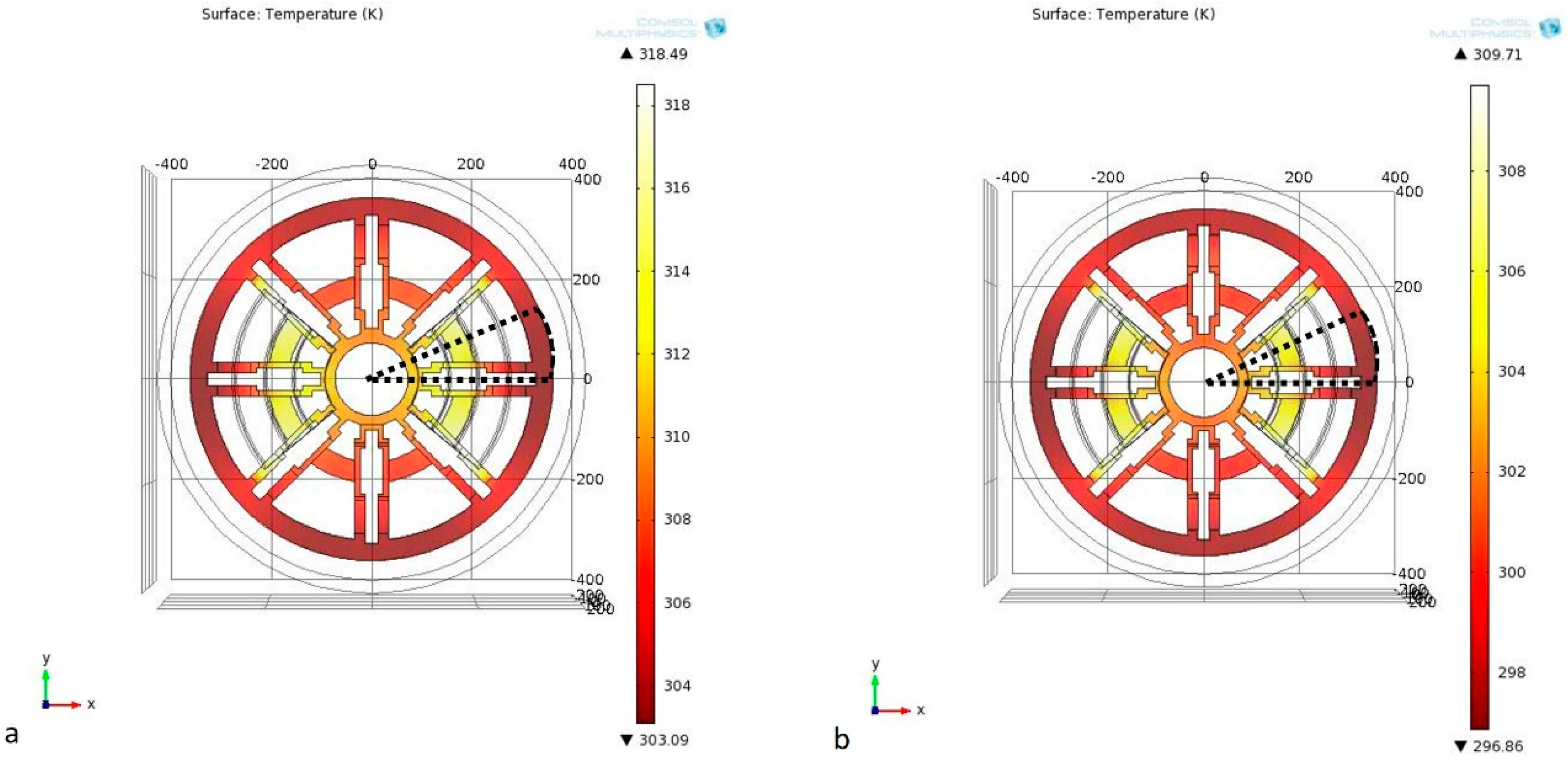
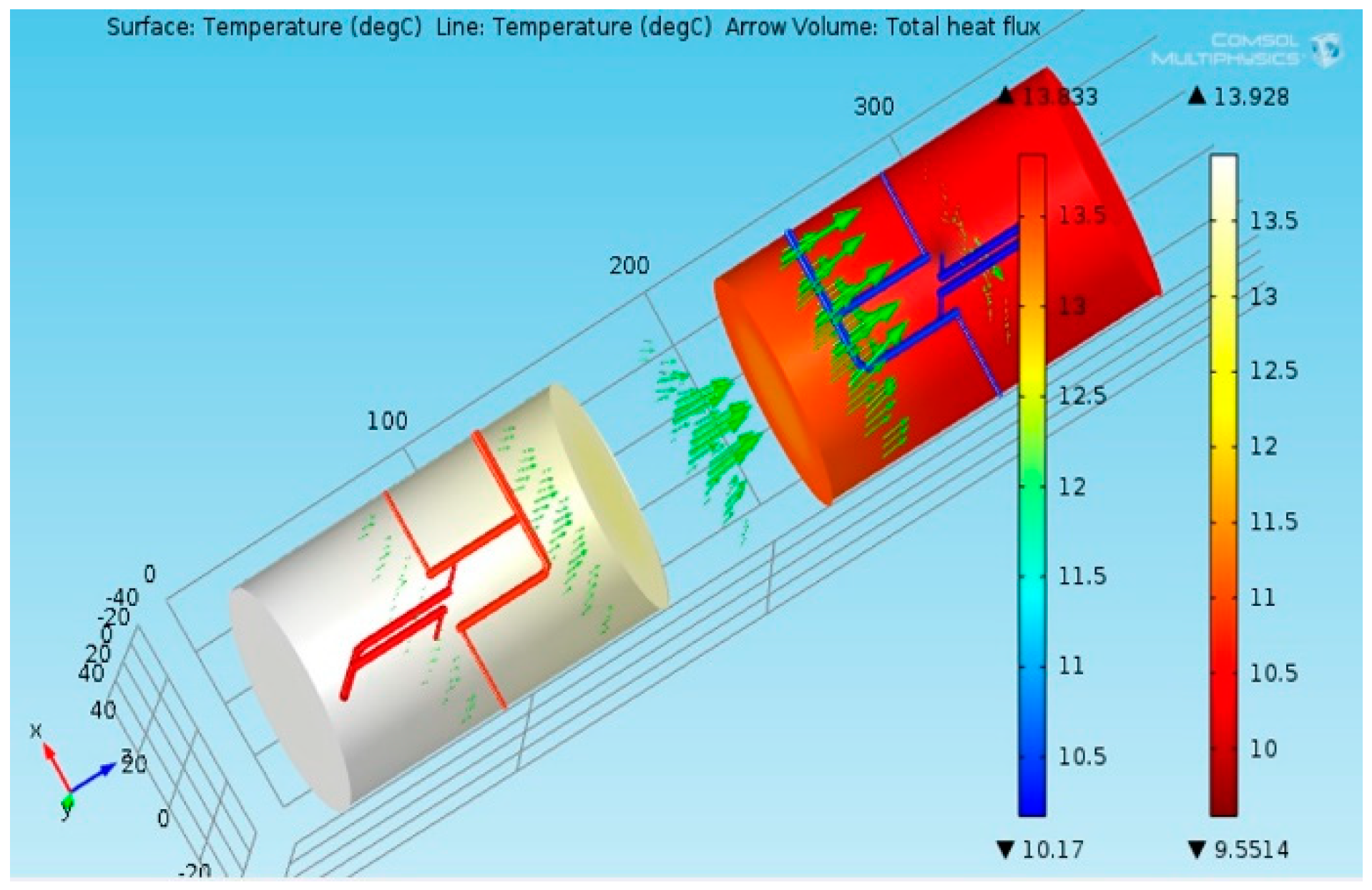
3.1.3. Stationary Thermal Model

After evaluating the distribution of eddy currents on the MCW, a steady-state 3D thermal sub-model was implemented, starting from the resistive losses field as a heat generation term. It was assumed that convective and radiative heat exchange can be described by an equivalent constant convective coefficient term on the whole domain to simplify the computation. Indeed, the purpose of the simulation is to validate the order of magnitude of the resistive losses previously calculated. Even if the problem is not completely stationary due to the dynamic behaviour of the system, it was assumed that a global heat flux invests the MCW. This global heat flux is the spatial composition of different heat flux for various β values. Hence, different steady-state simulations were performed for different angular positions. A single position of the magnetic assembly and a single portion of MCW was considered to validate the model.
The heat transfer through the MCW is described by a steady-state energy balance equation, as
· ( k T M C W ) =   q e c ,
where the heat source ( q e c ) is represented by the resistive losses due to eddy currents generation.
The heat dissipated on air-exposed surfaces is equal to
n · q = h ( T a i r     T M C W ) ,
where h is the equivalent heat transfer coefficient, supposed constant on the whole surface.
Since the magnets rotate, forced convection can be assumed depending on the magnets angular speed. In the analysed rotating frequency range, h resulted to be within 20 and 30 W m−2 K−1, considering the following experimental correlation for the convective heat transfer coefficient ( h c ) expressed in W m−2 K−1, as a function of the rotating frequency f (in Hz)
h c = 10.45 f + 10 f 0.5 .
In Figure 6, the surface temperature of the MCW is shown for an ambient temperature of 20 °C and a rotating frequency equal to 0.72 Hz. The regenerator place mostly permeated by the magnetic field has been taken as reference for temperature increase validation.
The value of the power dissipated by generation of eddy currents can be assumed as
W ˙ e c = Q ˙ e c .

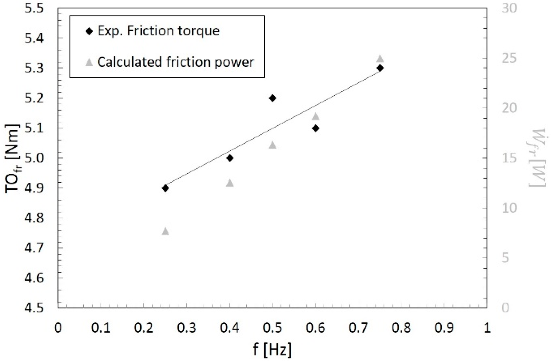
3.1.4. Semi-Empirical Evaluation of Friction Losses

The identification of the resistant torque concerning the friction effects into the rotary valve ( T o f r ( ω ) ) was performed by a semi-empirical approach that allowed to identify the relation between the friction resistant losses and the operating frequency ( f ), expressed by Equation (20).
T O f r ( ω ) = 0.7586 f + 4.7207 = 0.7586 ω 60 + 4.7207 .
In Figure 7, the results of the experimental measurements of the resistant torque without the MCW and the regenerators used to point out Equation (20) are shown.
The power dissipated due to friction effects was easily calculated as
W ˙ f r ( ω ) = 2 π f T O f r ( ω ) .
However, the reduction of friction losses is not considered in this work as a possible improvement for ‘8MAG’ since they are negligible compared to the energy losses concerning eddy currents generation.

3.2. Thermal Model

The rotary valve is subjected to a heat exchange between its external surface and the surrounding air due to the temperature difference. Furthermore, an axial heat exchange occurs within the valve since the hot and cold sub-valve achieve different steady-state temperature levels during cyclic operations of ‘8MAG’. This temperature difference between the sub-valves is only related to the fluid flow through the internal ducts of the valve.
Considering the surface of the cold sub-valve, it is possible to identify an axial conductive thermal loss though the hot buffer of the valve ( Q ˙ a x i a l ) and a convective radiative heat loss on the external surface ( Q ˙ s u r f ). Hence, the parasitic heat loss can be evaluated with the equation
Q ˙ c , l o s s = Q ˙ s u r f + Q ˙ a x i a l .
A FEM analysis, based on a 3D steady-state thermal model, was performed to evaluate the intrinsic thermal load of the rotary valve. A 3D geometrical model of the rotary valve was developed whereas the internal water ducts were modelled as 1D channel thermally coupled to the geometry of the valve (see Figure 8).
As made for the mechanical model, the domain was first defined considering the real geometry of the rotary valve. Then, the geometry was simplified to reduce computational time, neglecting geometrical singularities and complex details of low relevance. The entire geometry was included in a cylindrical volume with a diameter equal to 2.5 times of the diameter of the rotary valve and a height equal to 2.5 times of the height of the entire valve. Three different mesh were testes: coarser (12,045 elements), normal (23,615 elements), and extremely fine (922,712 elements). Analysing the standard deviation of Q ˙ c , l o s s , the normal mesh was chosen as the best.
The following equations were solved for the 1D water flux
· ( A ρ u w ) = 0 ,
p + f D ρ 2 D h u w | u w | = 0 ,
where u is the average surface velocity, ρ is the water density, p is the water pressure, D h is the equivalent diameter, f D is the Darcy friction coefficient, calculated with Churchill equation. In Equation (25), the energy balance equation is also shown as
ρ A c p u w · T w = · A k T w + f D ρ A 2 D h | u w | u w 2 + Q ˙ w a l l ,
where c p is the specific heat at constant pressure, T w is the water temperature and k is the thermal conductivity. Q ˙ w a l l represents heat through pipe surface, which is equal to
Q ˙ w a l l = h i n t Z   ( T e x t T w ) ,
where Z is the perimeter of the duct, h i n t is the internal heat exchange coefficient, T e x t is the external temperature of the pipe, which corresponds to the temperature of the solid ( T s ).
The temperature field inside the valve is governed by the equation
· ( k T s ) = 0 ,
where T s is the solid temperature. The boundary conditions are represented by Equations (28) and (29)
n · ( k T s ) = h a i r ( T a i r T s u r f ) ,
n · ( k T s ) = 0 ,
where h a i r is the convective heat transfer coefficient, T a i r is the temperature of the air surrounding the rotary valve and T s u r f is the valve surface temperature. End parts of the valve are assumed to be adiabatic. Solving the equations reported above, the thermal model allows to carry out the two components of Q ˙ c , l o s s , that are Q ˙ s u r f and Q ˙ a x i a l , and therefore to quantify the parasitic thermal losses in the rotary valve. The latter information is very useful since can help to understand which improvements can be made on the prototype to increase its overall performance.

4. Model Validation

The models introduced in Section 3 were validated by experimental tests for different working conditions, in terms of hot source temperature ( T H ), operating frequency ( f ) and volumetric flow rate ( V ˙ ). Only experimental tests at zero load were considered for model validation.

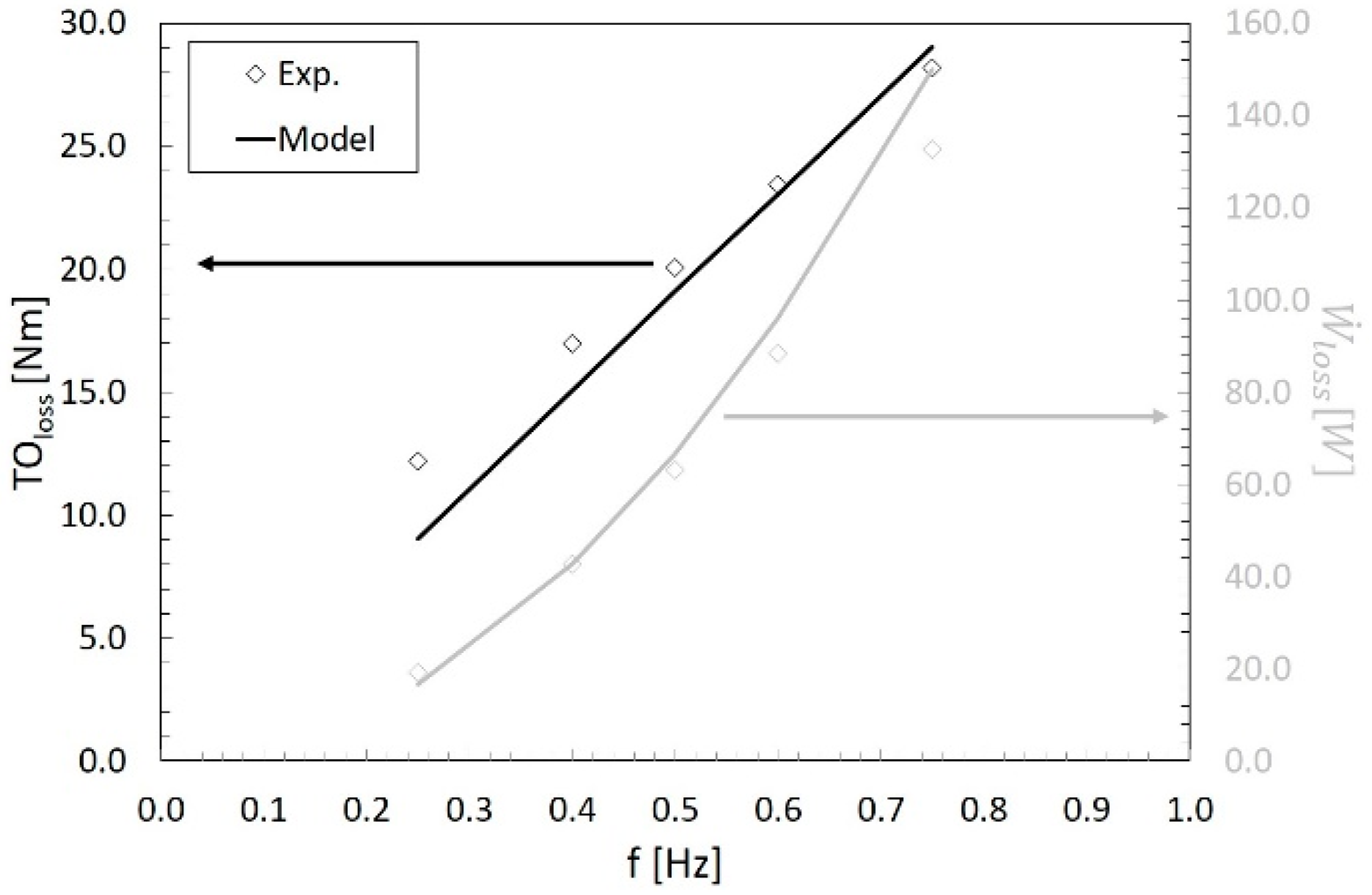
4.1. Mechanical Model Validation

To evaluate the performance of the mechanical model, it was required to validate only the sub-models used to calculate W ˙ e c (SMF, SECP, and ST) since W ˙ f r was estimated by a semi-empirical method (see Section 3.1.4).
The validation of the SMF sub-model was performed by carrying out some experimental measurements of the magnetic field by fixing a magnetometer on a radial axis and rotating step-by-step the magnets for different angular position β. The experimental results were then compared with the simulation in terms of the z component of the magnetic flux density Bz. A good agreement was found between experiments and simulation, highlighting that the model can reproduce magnetic field distribution, peaks, and valleys. Locally comparing measured and simulated data, a narrow absolute error emerged (−0.09 T), whereas the maximum relative error is of about 15%. The comparison between experiments and simulation of some representative points is shown in Table 2.
The calculated error values are acceptable considering the accuracy of the used instrumentation.
The SECP sub-model was validated measuring at different operating frequencies the resistant torque to the drive shaft with the MCW and removing all regenerators to exclude the term T O g d from Equation (1). Hence, the measured torque is composed only by the friction term ( T O f r ) and the eddy currents component ( T O e c ). On the other hand, the related measured mechanical power represents the mechanical power losses W ˙ l o s s . The experimental data of resistant torque (indicated as T O l o s s ) and mechanical power ( W ˙ l o s s ) were used to make a comparison with the simulation data obtained by the SECP model. Since the SECP model does not consider friction effects, the simulation results, in terms of T O e c , were increased with the friction losses contribution calculated with the semi-empirical model (see Equations (20) and (21)).
Hence, the comparison between the simulated and experimental resistant torque is shown in Figure 9, as well as the mechanical power loss. There is a good agreement between the measurements and the simulation results, with an average relative deviation of about 8.0% in the mechanical power (comparing the grey full line and grey symbols). This value is considered acceptable for the aim of this study. The greatest deviation in the mechanical power can be observed at f = 0.75 Hz. On the other hand, the simulated torque data (black full line) follow the trend of the experimental ones (black symbols) showing larger deviations for lower frequencies.
The ST model was validated comparing simulated data with experimental temperature measurements performed at different operating frequencies without regenerators and water flowing through the system. Six thermo-resistances, properly insulated, were placed on different representative positions on the metal surface of the MCW (see Figure 10).
Then, the surface temperature distribution of the MCW was obtained by the ST model and the simulated temperatures at the same position of Figure 10 were extracted. The comparison between the experimental and simulated temperature is shown in Figure 11.
The resulting value of the mean absolute percentage error (MAPE) is 4.0% with a maximum relative error of +7.8%, occurred for T3 (yellow line). These error values are considered acceptable for the aim of this work since are very close to the error range of the used instrumentation. The validation of the ST model demonstrates the capability of the mechanical model of providing a good estimation of the eddy current losses of ‘8MAG’, which can be used to evaluate its achievable performance after their reduction.

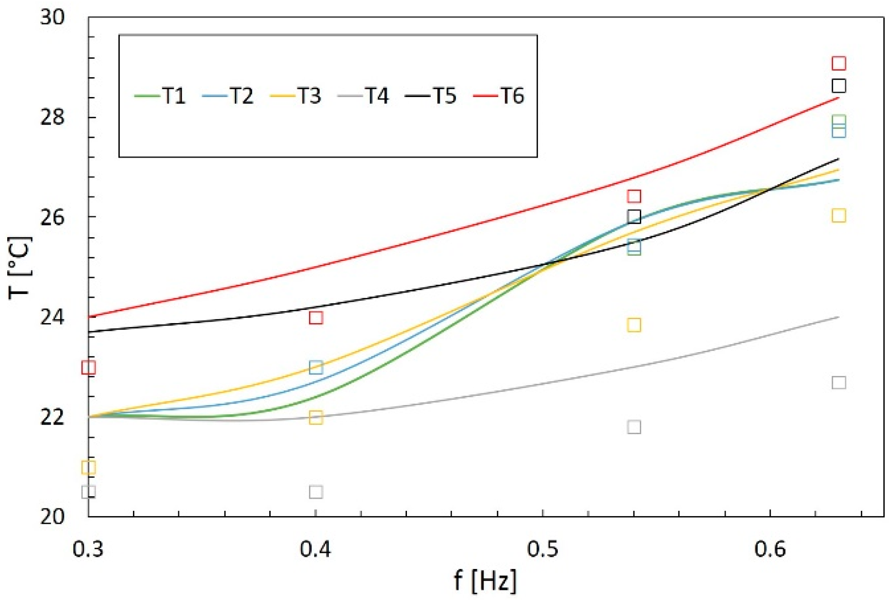
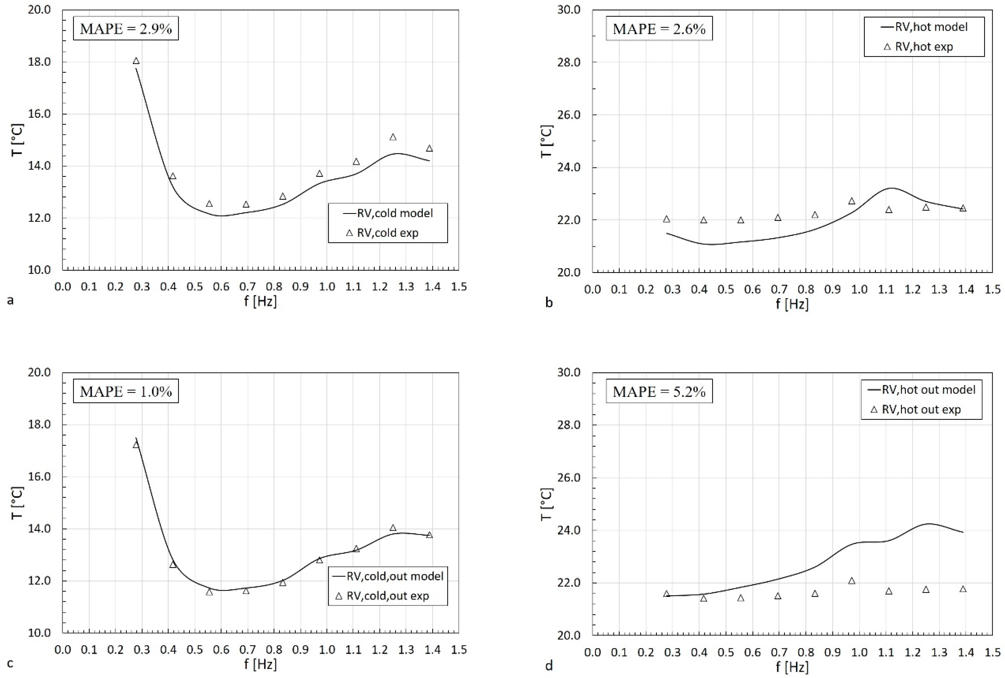
4.2. Thermal Model Validation

To validate the thermal model, sub-valves outlet water temperatures (cold sub-valve ( T R V , C , o u t ) and hot sub-valve ( T R V , H , o u t )) and their surface temperatures (cold sub-valve ( T R V , C ) and hot sub-valve ( T R V , H )) have been measured and compared to model results for different operating conditions. An example of simulation results is reported in Figure 12 where the temperature distribution and heat flux are shown.
In Figure 13, the comparison between the experimental and simulation results for the four temperatures mentioned above is reported. The value of the MAPE between simulation and experimental results is also shown for each temperature.
The values of the relative error range and the maximum absolute error for each temperature are shown in Table 3. A maximum relative error of +11.4% occurs regarding T R V , H , o u t . This large error could be related to the adiabatic surface hypothesis of the end parts of the rotary valve. However, these error values are considered acceptable considering the aim of this study.
In Figure 14, an example of result from the thermal model is shown. In detail, the parasitic thermal load Q ˙ c , l o s s is evaluated as a function of the operating frequency ( f ) and hot source temperature ( T H ). It is worth to notice that the parasitic thermal load presents a paraboloid shape with a maximum of about 61 W at an operating frequency of 0.8 Hz and T H equal to 23 °C.

5. Results and Discussion

The models developed in this work can help to quantify the main energy losses of ‘8MAG’, and therefore to evaluate the performance which the prototype can achieve reducing at the minimum these losses. Before evaluating the achievable performance, a comprehensive energy characterization of ‘8MAG’ was performed. In detail, cooling power, absorbed power and temperature span were measured for several operating conditions [15]. Then, it was possible to calculate the reference performance of the system, that is the coefficient of performance (COP), defined as
C O P r e f = Q ˙ c W ˙ t o t + W ˙ p u m p .
The uncertainty of COP, measured by error propagation rules for indirect measurements, was estimated to ±0.28%.
Figure 15 shows the ‘8MAG’ COP for different operating conditions, in terms of volumetric flow rate ( V ˙ ), measured in L min−1, and operating frequency ( f ) for three different levels of cooling power (50 W, 100 W, and 200 W) at a hot source temperature of 22 °C. From Figure 15, it is evident that COP decreases with the operating frequency increasing (at a constant cooling power) since the mechanical power required to move the magnets increases. The same trend can be noticed also considering the volumetric flow rate, even if it is less marked. However, the experimental tests showed that ‘8MAG’ can achieve a maximum COP of about 2.5 with a cooling power equal to 200 W and a temperature span of 2 K. These results represent the baseline of the ‘8MAG’ performance and they are used as a comparison to evaluate the possible improvements which could be achieved reducing the mechanical and thermal losses calculated by the models described in Section 3, regarding eddy currents and intrinsic thermal load of the rotary valve.

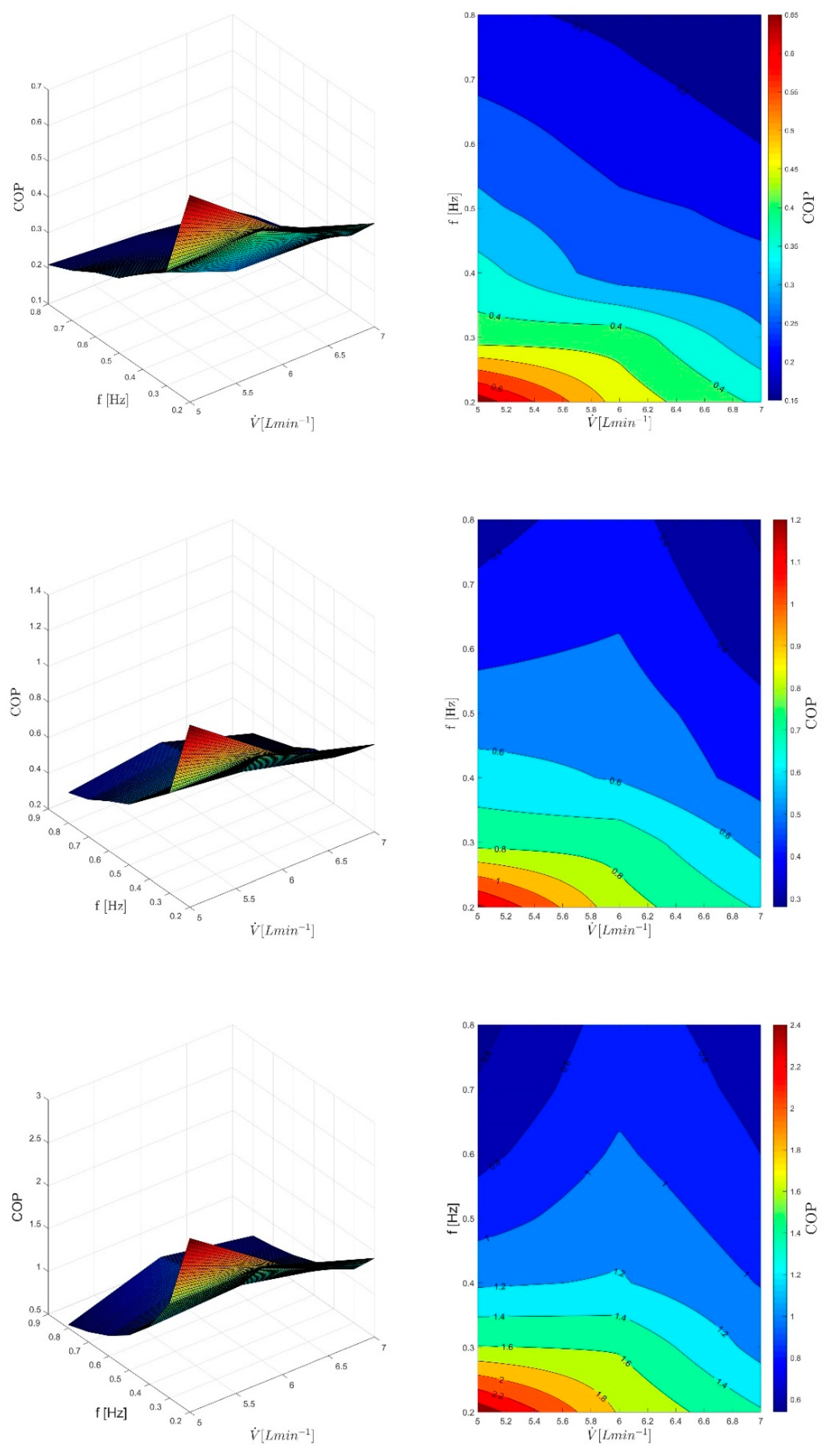
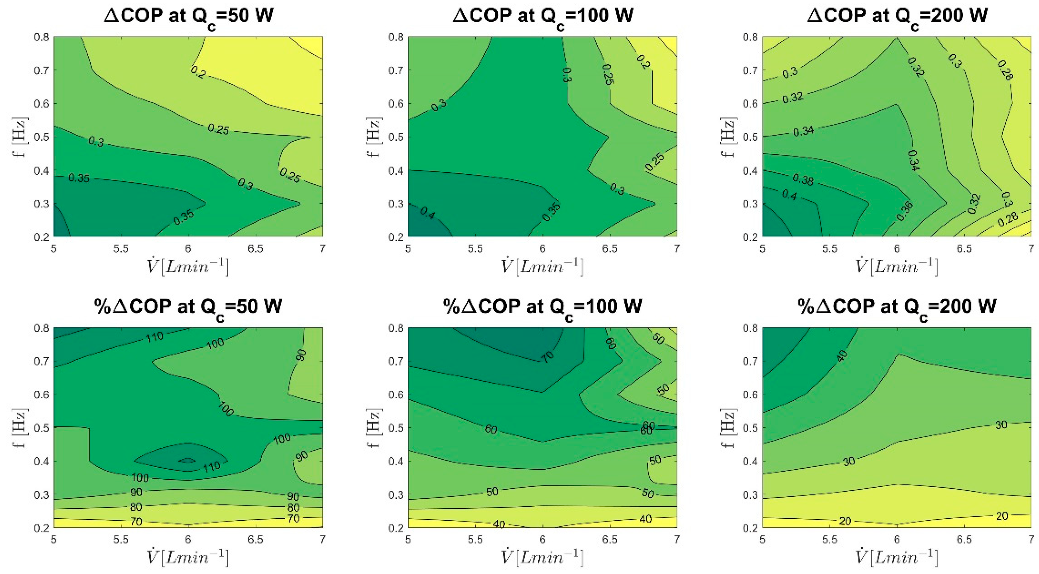
5.1. COP Improvement by Reducing Eddy Currents

The mechanical model allowed evaluating energy losses related to eddy currents generation in the MCW. These energy losses could be reduced by substituting the material of the MCW (or removing it). Hence, the new COP ( C O P e c ) can be calculated as
C O P e c = Q ˙ c ( W ˙ t o t W ˙ e c ) + W ˙ p u m p ,
where W ˙ e c represents the mechanical power recovered by reducing eddy currents. In Figure 16, the COP improvement obtained with this solution is shown, both in absolute (ΔCOP) and relative (% ΔCOP) terms. It was calculated according to Equations (32) and (33).
Δ C O P = C O P e c C O P r e f ,
% Δ C O P = C O P e c C O P r e f C O P r e f .
It is evident that the COP improvement strongly depends on the cooling power ( Q ˙ c ), the operating frequency ( f ) and the volumetric flow rate ( V ˙ ). As expected, the reduction of eddy currents leads to improve the ‘8MAG’ performance for each operating condition. In detail, the improvement is more pronounced for higher cooling power, with a maximum COP increase of about 0.60, whereas it is about 0.18 with a cooling power of 50 W. Furthermore, it is worth to notice that the COP increase is more evident at higher operating frequencies, as one can see from the relative variation of COP (bottom plots in Figure 16).

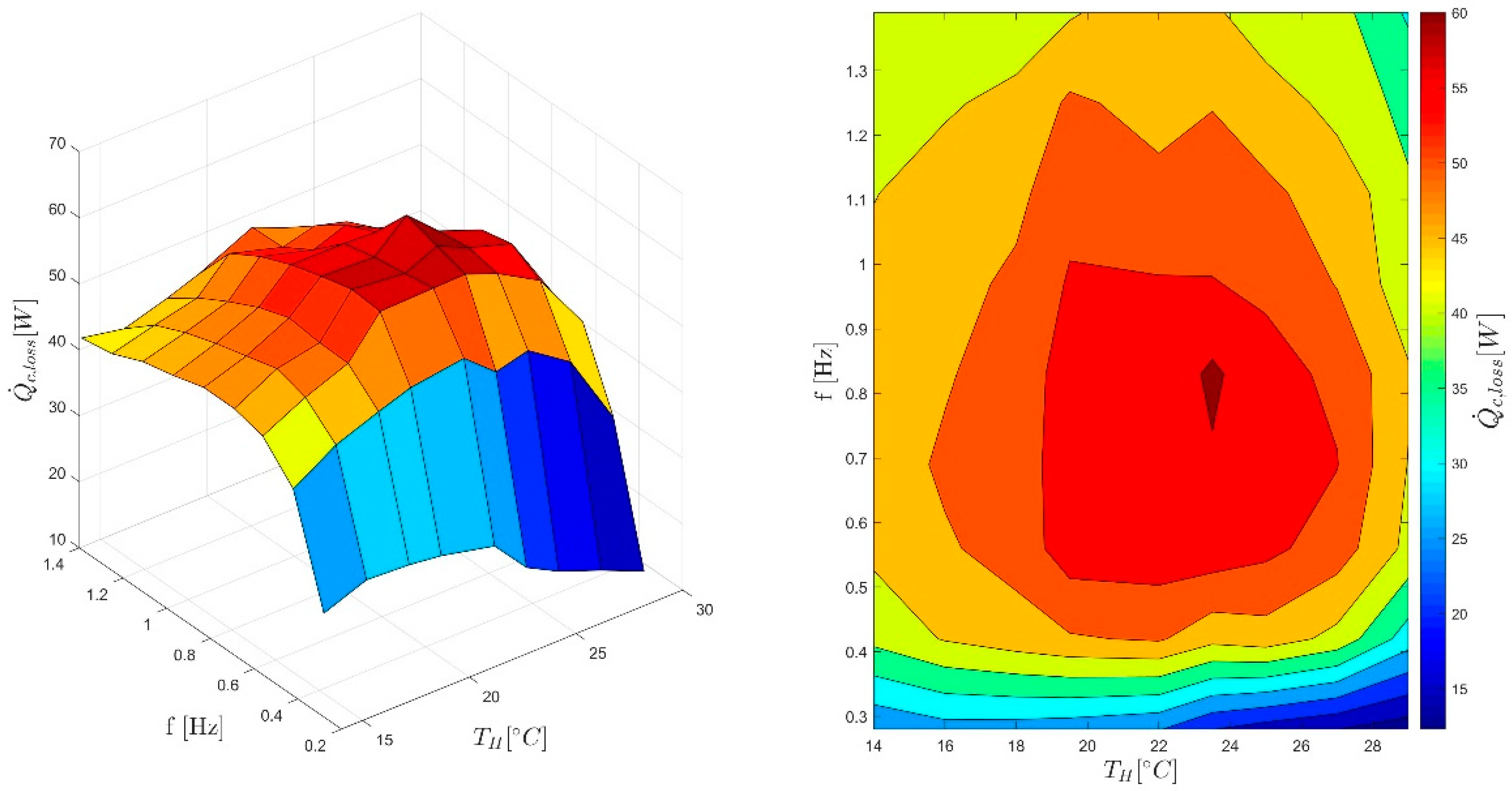
5.2. COP Improvement by Reducing Parasitic Thermal Load

Using the thermal model, it was possible to evaluate the parasitic thermal load of the rotary valve, which is related to its non-adiabatic characteristic. Considering an ideal adiabatic rotary valve, and therefore trying to improve the insulation of this component, these thermal losses could be reduced and a new COP ( C O P Q c , l o s s ) can be found as
C O P Q c , l o s s = Q ˙ c + Q ˙ c , l o s s W ˙ t o t + W ˙ p u m p .
In Figure 17, the comparison between the actual COP of ‘8MAG’ and the theoretical COP obtainable reducing the parasitic thermal load of the rotary valve is shown for different operating conditions. The data reported in Figure 17 are calculated according to Equations (32) and (33), substituting C O P e c with C O P Q c , l o s s . It can be noticed that reducing the intrinsic thermal load of the rotary valve (improving its insulation) can improve the ‘8MAG’ COP of about 0.40. It is worth to consider that the improvement does not change so much by varying the cooling power, in contrast with the improvement observed by reducing eddy currents losses. Furthermore, in this case, the beneficial effect increases with decreasing the operating frequency of the device.

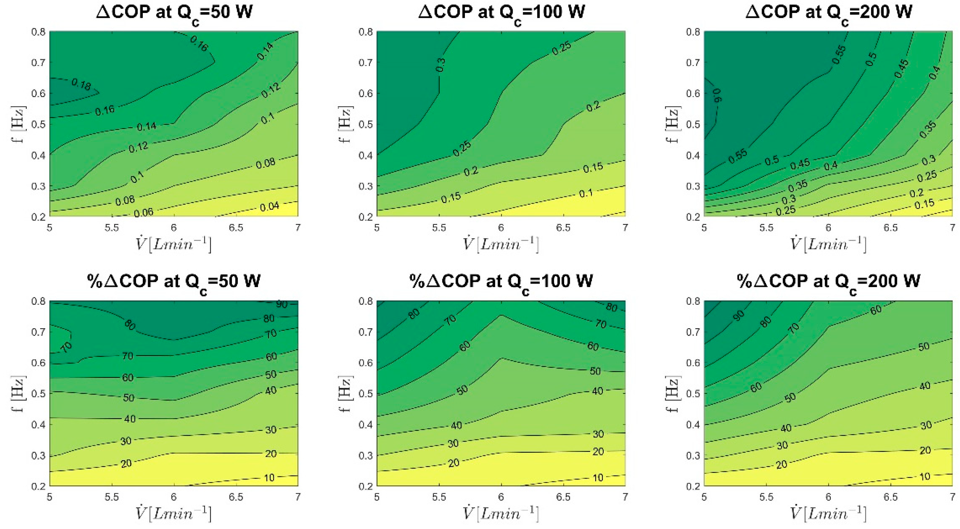
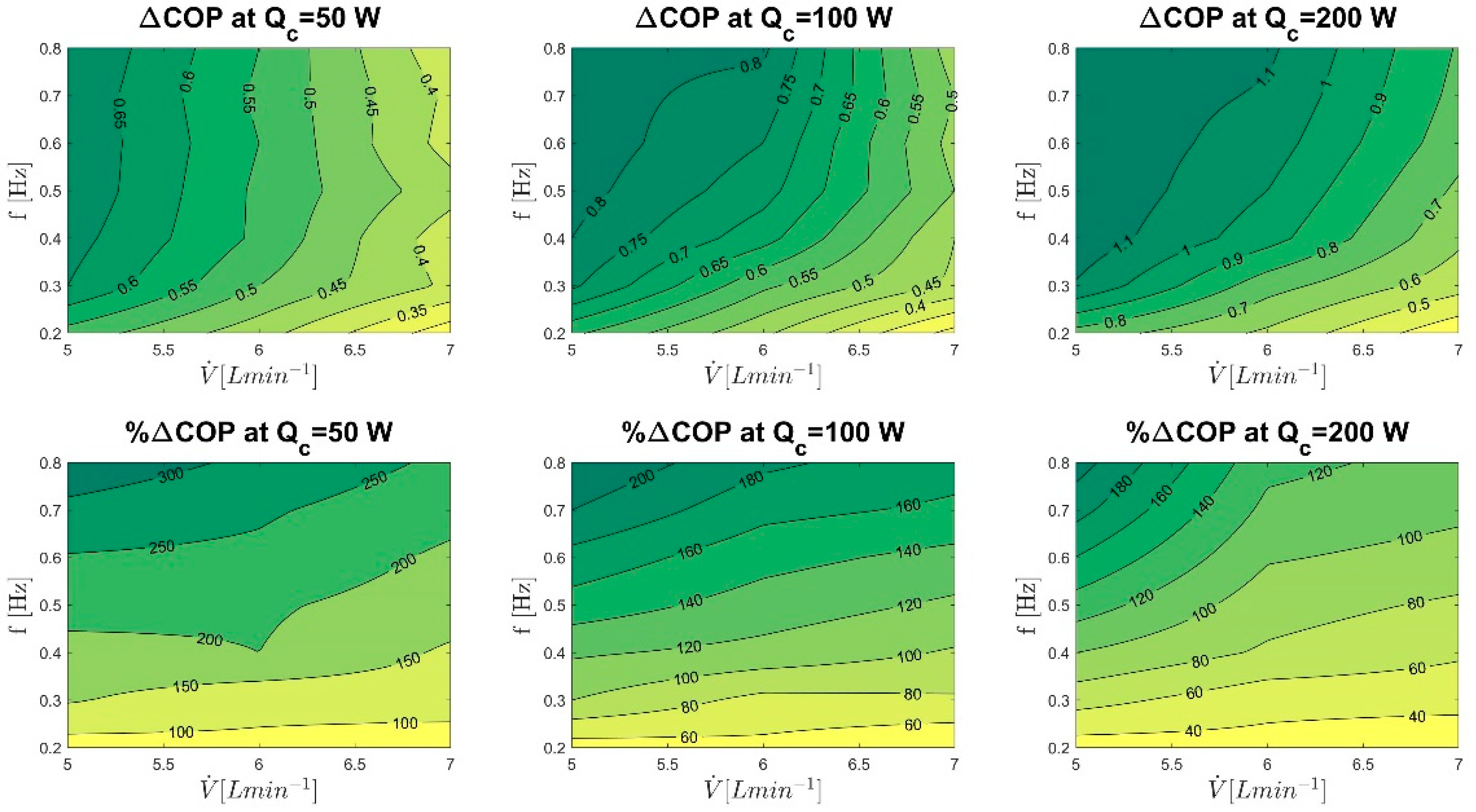
5.3. Overall Achievable COP Improvement

To complete the analysis, the effect of introducing both the previous improvements (reduction of eddy currents generation in the MCW by substitution of the material and refinement of the rotary valve insulation) is investigated. Hence, another COP value ( C O P e c + Q c , l o s s ) is calculated (see Equation (35)).
C O P e c + Q c , l o s s = Q ˙ c + Q ˙ c , l o s s ( W ˙ t o t W ˙ e c ) + W p u m p .
As performed in the previous sub-sections, the comparison between this new COP and the reference COP of the prototype is shown in Figure 16, according to Equations (32) and (33).
Figure 18 shows the best obtainable COP of ‘8MAG’ which can be achieved if both the energy losses investigated in this study are reduced. Hence, it represents the maximum improvements of the performance of ‘8MAG’ for different operating conditions. In detail, a maximum increase of about 1.1 is highlighted with a cooling power of 200 W at relatively high frequencies (higher than 0.3 Hz) and low volumetric flow rate (lower than 6 L min−1). Good improvements can be achieved also for lower cooling power, with maximum increases of the COP value of 0.65 and 0.8, with cooling power of 50 W and 100 W, respectively.
In Table 4, an overview of the results is shown, regarding the average, maximum, and minimum COP values in four different configurations, for three values of heat source temperature and cooling power. The average COP reported in Table 4 was calculated performing an average among all the COP values calculated at different operating frequencies and volumetric flow rates at the same heat source temperature and cooling power.
It is worth to highlight that the maximum ‘8MAG’ COP, starting from the actual value of 2.5, can achieve a value equal to 3.3 (+30.3%), if the energy losses evaluated in this work can be reduced. However, only substituting the material of the MCW (to reduce eddy currents generation) can increase the COP up to 2.8 (+10.9%) whereas a better insulation of the rotary valve can increase the COP up to 3.0 (+17.5%). On the other hand, the second-law efficiency, starting from the previous maximum value of 2.4%, can achieve a value equal to 3.5% (+46%) at TH = 16 °C and a temperature span of 4.7 K, if the energy losses evaluated in this work can be reduced.

6. Conclusions

In this study, the main energy losses of a rotary permanent magnet magnetic refrigerator, named ‘8MAG’, developed at University of Salerno, were investigated with the aim to estimate the achievable performance of such a system. In detail, starting from the design details of the prototype, two different kinds of losses were identified: mechanical losses, regarding eddy currents generation inside the MCW and friction phenomena in the rotary valve, and parasitic thermal losses, related to the non-adiabatic conditions of the rotary valve.
Mechanical and thermal losses were investigated by developing two uncoupled models: the mechanical model, divided into three sub-models (SMF, SECP, and ST), which allowed to identify the power dissipated by eddy currents generation, and the thermal model, which could point out the parasitic heat load of the rotary valve. The mechanical power dissipated by friction phenomena was estimated by a semi-empirical model, based on experimental measurements and datasheets of the rotary valve components. The mechanical and thermal model were validated with experimental data, showing a good agreement with a maximum relative error of +8.0% and +11.4%, respectively. These models were developed for estimating only the main losses of the prototype to analyse the hypothetical achievable COP, and they do not consider the effect of temperature span, or even of the heat exchange between the MCW and regenerators, which could also affect the performance of the system.
Using the mechanical model, eddy currents losses were calculated for different operating conditions and maximum COP improvements were estimated within the range from 0.1 (with a cooling power of 50 W) to 0.3 (with a cooling power of 200 W). On the other hand, the reduction of parasitic heat losses, estimated by the thermal model, could lead to a maximum COP increase of about 0.5, showing a lower dependence on cooling power than eddy current losses. Reducing both eddy currents and parasitic heat losses, a greater improvement can be achieved, with a maximum COP increase of 0.8, which allows to reach a COP value of 3.3 (+32.0% against the reference value of 2.5). This increment allows ‘8MAG’ to get closer to other magnetic refrigerator prototypes presented in the literature, in terms of performance. In detail, the improved ‘8MAG’ performance are closer to the best performance showed so far by a magnetic refrigerator prototype (COP of 5 with a temperature span of 5 K), with a difference of 1.7 against 2.5 of ‘8MAG’ without improvements.
The potential COP improvements showed in this study can be achieved on the real device by two actions: changing the aluminium of the MCW with another material with a lower electrical conductivity to reduce eddy currents generation and enhancing the insulation of the rotary valve to reduce parasitic heat losses. Future works could deal with experimental tests with the upgraded system, to test the actual performance improvement, and the analysis of other kinds of energy losses.

Author Contributions

A.M. (Angelo Maiorino) conceived the idea and helped with the discussion of the results and the model development. A.M. (Antongiulio Mauro) developed the model, performed experimental measurements, analysed experimental data and wrote some parts of the paper (when he was a Ph.D. candidate at University of Salerno). M.G.D.D. wrote some parts of the paper, prepared figures and helped with the discussion of the results. A.M.-B. helped with the discussion of results. C.A. supervised the entire work.

Funding

This research received no external funding.

Acknowledgments

Adrián Mota-Babiloni would like to thank the financial support from the Spanish Government through the postdoctoral contract Juan de la Cierva-Formación 2016 (ref. FJCI-2016-28324), and Banco Santander and Universitat Jaume I for the mobility grant “Becas Iberoamérica. Santander Universidades. Convocatoria 2018/2019”.

Conflicts of Interest

The authors declare no conflict of interest.

References

  1. Barclay, J.A. Theory of an Active Magnetic Regenerative Refrigerator. United States. Available online: https://www.osti.gov/servlets/purl/6224820 (accessed on 26 July 2019).
  2. Steven Brown, J.; Domanski, P.A. Review of alternative cooling technologies. Appl. Therm. Eng. 2014, 64, 252–262. [Google Scholar] [CrossRef]
  3. Rowe, A. Thermodynamics of active magnetic regenerators: Part I. Cryogenics 2012, 52, 111–118. [Google Scholar] [CrossRef]
  4. Rowe, A. Thermodynamics of active magnetic regenerators: Part II. Cryogenics 2012, 52, 119–128. [Google Scholar] [CrossRef]
  5. Aprea, C.; Greco, A.; Maiorino, A.; Masselli, C. The environmental impact of solid-state materials working in an active caloric refrigerator compared to a vapor compression cooler. Int. J. Heat Technol. 2018, 36, 1155–1162. [Google Scholar] [CrossRef]
  6. Aprea, C.; Greco, A.; Maiorino, A.; Masselli, C. Magnetic refrigeration: An eco-friendly technology for the refrigeration at room temperature. J. Phys. Conf. Ser. 2015, 655, 012026. [Google Scholar] [CrossRef]
  7. Greco, A.; Aprea, C.; Maiorino, A.; Masselli, C. A review of the state of the art of solid-state caloric cooling processes at room-temperature before 2019. Int. J. Refrig. 2019, 106, 66–88. [Google Scholar] [CrossRef]
  8. Yu, B.; Liu, M.; Egolf, P.W.; Kitanovski, A. A review of magnetic refrigerator and heat pump prototypes built before the year 2010. Int. J. Refrig. 2010, 33, 1029–1060. [Google Scholar] [CrossRef]
  9. Engelbrecht, K.; Pryds, N. Progress in magnetic refrigeration and future challenges. In Proceedings of the 6th IIF-IIR International Conference on Magnetic Refrigeration. International Institute of Refrigeration, Victoria, BC, Canada, 7–10 September2014. [Google Scholar]
  10. Lozano, J.A.; Engelbrecht, K.; Bahl, C.R.H.; Nielsen, K.K.; Eriksen, D.; Olsen, U.L.; Barbosa, J.R.; Smith, A.; Prata, A.T.; Pryds, N. Performance analysis of a rotary active magnetic refrigerator. Appl. Energy 2013, 111, 669–680. [Google Scholar] [CrossRef]
  11. Rowe, A. Configuration and performance analysis of magnetic refrigerators. Int. J. Refrig. 2011, 34, 168–177. [Google Scholar] [CrossRef]
  12. Rosario, L.; Rahman, M.M. Analysis of a magnetic refrigerator. Appl. Therm. Eng. 2011, 31, 1082–1090. [Google Scholar] [CrossRef]
  13. Romero Gómez, J.; Ferreiro Garcia, R.; Carbia Carril, J.; Romero Gómez, M. Experimental analysis of a reciprocating magnetic refrigeration prototype. Int. J. Refrig. 2013, 36, 1388–1398. [Google Scholar] [CrossRef]
  14. Lozano, J.A.; Engelbrecht, K.; Bahl, C.R.H.; Nielsen, K.K.; Barbosa, J.R.; Prata, A.T.; Pryds, N. Experimental and numerical results of a high frequency rotating active magnetic refrigerator. Int. J. Refrig. 2014, 37, 92–98. [Google Scholar] [CrossRef]
  15. Aprea, C.; Greco, A.; Maiorino, A.; Masselli, C. The energy performances of a rotary permanent magnet magnetic refrigerator. Int. J. Refrig. 2016, 61, 1–11. [Google Scholar] [CrossRef]
  16. Aprea, C.; Greco, A.; Maiorino, A.; Mastrullo, R.; Tura, A. Initial experimental results from a rotary permanent magnet magnetic refrigerator. Int. J. Refrig. 2014, 43, 111–122. [Google Scholar] [CrossRef]
  17. Lozano, J.A.; Capovilla, M.S.; Trevizoli, P.V.; Engelbrecht, K.; Bahl, C.R.H.; Barbosa, J.R. Development of a novel rotary magnetic refrigerator. Int. J. Refrig. 2016, 68, 187–197. [Google Scholar] [CrossRef]
  18. Eriksen, D.; Engelbrecht, K.; Bahl, C.R.H.; Bjørk, R.; Nielsen, K.K.; Insinga, A.R.; Pryds, N. Design and experimental tests of a rotary active magnetic regenerator prototype. Int. J. Refrig. 2015, 58, 14–21. [Google Scholar] [CrossRef]
  19. Huang, B.; Lai, J.W.; Zeng, D.C.; Zheng, Z.G.; Harrison, B.; Oort, A.; van Dijk, N.H.; Brück, E. Development of an experimental rotary magnetic refrigerator prototype. Int. J. Refrig. 2019, 104, 42–50. [Google Scholar] [CrossRef]
  20. Albertini, F.; Bennati, C.; Bianchi, M.; Branchini, L.; Cugini, F.; De Pascale, A.; Fabbrici, S.; Melino, F.; Ottaviano, S.; Peretto, A.; et al. Preliminary Investigation on a Rotary Magnetocaloric Refrigerator Prototype. Energy Procedia 2017, 142, 1288–1293. [Google Scholar] [CrossRef]
  21. Gimaev, R.; Spichkin, Y.; Kovalev, B.; Kamilov, K.; Zverev, V.; Tishin, A. Review on magnetic refrigeration devices based on HTSC materials. Int. J. Refrig. 2019, 100, 1–12. [Google Scholar] [CrossRef]
  22. Plaznik, U.; Tušek, J.; Kitanovski, A.; Poredoš, A. Numerical and experimental analyses of different magnetic thermodynamic cycles with an active magnetic regenerator. Appl. Therm. Eng. 2013, 59, 52–59. [Google Scholar] [CrossRef]
  23. Kitanovski, A.; Plaznik, U.; Tušek, J.; Poredoš, A. New thermodynamic cycles for magnetic refrigeration. Int. J. Refrig. 2014, 37, 28–35. [Google Scholar] [CrossRef]
  24. Lucia, U. General approach to obtain the magnetic refrigeretion ideal coefficient of performance. Phys. A Stat. Mech. Its Appl. 2008, 387, 3477–3479. [Google Scholar] [CrossRef]
  25. Trevizoli, P.V.; Nakashima, A.T.; Peixer, G.F.; Barbosa, J.R. Évaluation de la performance d’un régénérateur magnétique actif pour les applications de refroidissement—Partie I: Analyse expérimentale et performance thermodynamique. Int. J. Refrig. 2016, 72, 192–205. [Google Scholar] [CrossRef]
  26. Aprea, C.; Greco, A.; Maiorino, A.; Masselli, C. A comparison between rare earth and transition metals working as magnetic materials in an AMR refrigerator in the room temperature range. Appl. Therm. Eng. 2015, 91, 767–777. [Google Scholar] [CrossRef]
  27. Aprea, C.; Greco, A.; Maiorino, A. A dimensionless numerical analysis for the optimization of an active magnetic regenerative refrigerant cycle. Int. J. Energy Res. 2013, 37, 1475–1487. [Google Scholar] [CrossRef]
  28. Gao, X.Q.; Shen, J.; He, X.N.; Tang, C.C.; Li, K.; Dai, W.; Li, Z.X.; Jia, J.C.; Gong, M.Q.; Wu, J.F. Improvements of a room-temperature magnetic refrigerator combined with Stirling cycle refrigeration effect. Int. J. Refrig. 2016, 67, 330–335. [Google Scholar] [CrossRef]
  29. He, X.N.; Gong, M.Q.; Zhang, H.; Dai, W.; Shen, J.; Wu, J.F. Design and performance of a room-temperature hybrid magnetic refrigerator combined with Stirling gas refrigeration effect. Int. J. Refrig. 2013, 36, 1465–1471. [Google Scholar] [CrossRef]
  30. Aprea, C.; Greco, A.; Maiorino, A. GeoThermag: A geothermal magnetic refrigerator. Int. J. Refrig. 2015, 59, 75–83. [Google Scholar] [CrossRef]
  31. Lucas, C.; Koehler, J. Experimental investigation of the COP improvement of a refrigeration cycle by use of an ejector. Int. J. Refrig. 2012, 35, 1595–1603. [Google Scholar] [CrossRef]
  32. Aprea, C.; Greco, A.; Maiorino, A. An application of the artificial neural network to optimise the energy performances of a magnetic refrigerator. Int. J. Refrig. 2017, 82, 238–251. [Google Scholar] [CrossRef]
  33. Qian, S.; Yuan, L.; Yu, J.; Yan, G. Variable load control strategy for room-temperature magnetocaloric cooling applications. Energy 2018, 153, 763–775. [Google Scholar] [CrossRef]
  34. Qian, S.; Yuan, L.; Yu, J. An online optimum control method for magnetic cooling systems under variable load operation. Int. J. Refrig. 2019, 97, 97–107. [Google Scholar] [CrossRef]
  35. Aprea, C.; Cardillo, G.; Greco, A.; Maiorino, A.; Masselli, C. A rotary permanent magnet magnetic refrigerator based on AMR cycle. Appl. Therm. Eng. 2016, 101, 699–703. [Google Scholar] [CrossRef]
  36. Lei, T.; Engelbrecht, K.; Nielsen, K.K.; Veje, C.T. Study of geometries of active magnetic regenerators for room temperature magnetocaloric refrigeration. Appl. Therm. Eng. 2017, 111, 1232–1243. [Google Scholar] [CrossRef] [Green Version]
  37. Arnold, D.S.; Tura, A.; Ruebsaat-Trott, A.; Rowe, A. Design improvements of a permanent magnet active magnetic refrigerator. Int. J. Refrig. 2014, 37, 99–105. [Google Scholar] [CrossRef]
  38. Monfared, B. Design and optimization of regenerators of a rotary magnetic refrigeration device using a detailed simulation model. Int. J. Refrig. 2018, 88, 260–274. [Google Scholar] [CrossRef]
  39. Li, Z.; Shen, J.; Li, K.; Gao, X.; Guo, X.; Dai, W. Assessment of three different gadolinium-based regenerators in a rotary-type magnetic refrigerator. Appl. Therm. Eng. 2019, 153, 159–167. [Google Scholar] [CrossRef]
  40. Klinar, K.; Tomc, U.; Jelenc, B.; Nosan, S.; Kitanovski, A. New frontiers in magnetic refrigeration with high oscillation energy-efficient electromagnets. Appl. Energy 2019, 236, 1062–1077. [Google Scholar] [CrossRef]
  41. Czernuszewicz, A.; Kaleta, J.; Kołosowski, D.; Lewandowski, D. Experimental study of the effect of regenerator bed length on the performance of a magnetic cooling system. Int. J. Refrig. 2019, 97, 49–55. [Google Scholar] [CrossRef]
  42. Capovilla, M.S.; Lozano, J.A.; Trevizoli, P.V.; Barbosa, J.R. Performance evaluation of a magnetic refrigeration system. Sci. Technol. Built Environ. 2016, 22, 534–543. [Google Scholar] [CrossRef]
Figure 1. Prototype core details in cross-section (a) and 3-D view of MCW (b): (1) permanent magnet assembly; (2) magnets support; (3) shaft-rotary valve combination; (4) regenerators; (5) magneto caloric wheel (MCW); (6) cold sub-valve and (7) hot sub-valve.
Energies 12 04388 g001
Figure 2. Representation of the mechanical model (a) and the thermal model (b).
Energies 12 04388 g002
Figure 3. Modelled geometries (a), domain of the simulations (b), and meshes of magnets and the MCW (c).
Energies 12 04388 g003
Figure 4. Configuration of the permanent magnets as Halbach array.
Energies 12 04388 g004
Figure 5. Magnetic flux distribution (ac), induced current density (bd), and resistive losses (bd) for two different positions of the magnets.
Energies 12 04388 g005
Figure 6. Temperature distribution on the MCW surface for a rotating frequency of 0.72 Hz, an ambient temperature of 20 °C and different heat transfer coefficients: 20 (a) and 30 (b) W m−2 K−1. In the figures, the area of interest for the simulation is evidenced (black dotted lines).
Energies 12 04388 g006
Figure 7. Experimental resistant torque by friction effects (left y-axis) and correlated power dissipated (right y-axis) for different operating frequency.
Energies 12 04388 g007
Figure 8. Representation of internal water ducts and the 3D geometry of the rotary valve.
Energies 12 04388 g008
Figure 9. Comparison between experimental (symbols) and simulation (full line) results of resistant torque (black symbols and full line on the left y-axis, only losses contribution) and mechanical power losses (grey symbols and full line on the right y-axis).
Energies 12 04388 g009
Figure 10. Temperature sensors positioning on the surface of the MCW. Sensors 1 and 2 were placed on the top and bottom surface of the MCW, respectively.
Energies 12 04388 g010
Figure 11. Surface temperature of the MCW in six different representative points as a function of operating frequency: experimental (symbols) vs. simulated (full lines) results.
Energies 12 04388 g011
Figure 12. An example of simulation results for a rotating frequency of 17 Hz (that corresponds to 1000 rpm) and for a hot source temperature TH of 22 °C.
Energies 12 04388 g012
Figure 13. Comparison of experimental measurements and model results of (a,b) surface temperatures of both sub-valves ( T R V , C , T R V , H ) and (c,d) outlet water temperatures ( T R V , C , o u t ,   T R V , H , o u t ) for TH = 22 °C and different operating frequency.
Energies 12 04388 g013
Figure 14. Parasitic thermal load of the rotary valve simulated by the thermal model with different operating frequencies and hot source temperatures.
Energies 12 04388 g014
Figure 15. COP of ‘8MAG’ as a function of volumetric flow rate and operating frequency at TH = 22 °C and different cooling power (50 W, 100 W, and 200 W, from the top to the bottom). Temperature spans are in the range between 1 K and 8.5 K.
Energies 12 04388 g015
Figure 16. ‘8MAG’ COP changing by reducing ECL on the MCW for different operating conditions at TH = 22 °C. Temperature spans are in the range between 1 K and 8.5 K.
Energies 12 04388 g016
Figure 17. ‘8MAG’ COP changing by reducing thermal losses in the rotary valve for different operating conditions at TH = 22 °C. Temperature spans are in the range between 1 K and 8.5 K.
Energies 12 04388 g017
Figure 18. ‘8MAG’ COP changing by reducing both thermal losses in the rotary valve and ECL on the MCW for different operating conditions at TH = 22 °C. Temperature spans are in the range between 1 K and 8.5 K.
Energies 12 04388 g018
Table 1. Measurement instruments used for the experimental tests.
MeasurementInstrument TypeAccuracy
TemperatureRTD 4 wires0.1 K
TorqueTorque transducer0.5%
Angular velocityOptical encoder0.01° s−1
Magnetic fieldHall probe0.4%
Water flowElectromagnetic flowmeter0.5%
Electrical powerElectromagnetic wattmeter0.2%
Table 2. Absolute and relative errors of the SMF model for some representative points.
X (cm)y (cm)Bz_sim (T)Bz_exp (T)Absolute Error (T)Relative Error (%)
01000.2970.350−0.053−15.1
0−180−1.270−1.180−0.0907.5
0−200−1.069−1.0850.020−1.5
−100−180−0.827−0.800−0.0303.4
−15000.0850.0750.01012.8
Table 3. Absolute and relative error of the thermal model.
T R V , C T R V , H T R V , C , o u t T R V , H , o u t
Relative error range (%)1.7–4.40.2–4.20.1–1.60.4–11.4
Absolute max error (°C)0.70.90.32.5
Table 4. Average ‘8MAG’ COP for different cooling power and hot source temperatures (TH). These values were obtained by an average among the experimental data at different volumetric flow rates and operating frequencies. Temperature spans are in the range between 1 K and 8.5 K.
COPrefCOPecCOPQc,lossCOPec+Qc,loss
TH [°C]AveMaxMinAveMaxMinAveMaxMinAveMaxMin
Q ˙ c = 50   W 160.350.680.150.450.750.290.611.080.250.791.190.46
28.6%10.3%93.3%74.3%58.8%66.7%125.7%75.0%206.7%
220.350.680.150.450.750.290.641.090.280.831.210.51
28.6%10.3%93.3%82.9%60.3%86.7%137.1%77.9%240.0%
320.380.690.150.490.790.280.641.040.260.851.250.48
28.9%14.5%86.7%68.4%50.7%73.3%123.7%81.2%220.0%
Q ˙ c = 100   W 160.661.220.280.831.350.520.941.640.371.181.820.70
25.8%10.7%85.7%42.4%34.4%32.1%78.8%49.2%150.0%
220.661.220.280.831.350.520.971.650.401.221.830.75
25.8%10.7%85.7%47.0%35.2%42.9%84.8%50.0%167.9%
320.751.350.370.951.510.641.021.660.561.331.870.99
26.7%11.9%73.0%36.0%23.0%51.4%77.3%38.5%167.6%
Q ˙ c = 200   W 161.522.530.891.812.801.211.832.961.112.183.281.51
19.1%10.7%36.0%20.4%17.0%24.7%43.4%29.6%69.7%
221.522.530.891.812.801.211.862.971.152.233.291.57
19.1%10.7%36.0%22.4%17.4%29.2%46.7%30.0%76.4%
321.581.971.211.832.221.441.862.261.472.162.541.76
15.8%12.7%19.0%17.7%14.7%21.5%36.7%28.9%45.5%

