Optimal Coordination of Wind Power and Pumped Hydro Energy Storage

Abstract

A study combining wind power with pumped hydro energy storage for the Jordanian utility grid is presented. Three solvers of the Matlab optimization toolbox are used to find the optimal solution for the cost of energy in a combined on-grid system. Genetic algorithm, simulated annealing (SA), and pattern search (PS) solvers are used to find the optimal solution. The GA solution of 0.0955388 $/kWh is economically feasible. This is 28.7% lower than the electricity purchased from the conventional utility grid. The discounted payback period to recover the total cost is 10.271 years. The suggested configuration is shown to be feasible by comparing it to real measurements for this case and a previous wind-only case. It is shown that the indicators of the optimal solution are improved. For instance, carbon dioxide emissions (E_CO2) and conventional grid energy purchases are reduced by 24.69% and 24.68%, respectively. Moreover, it is shown that the benefits of adding hydro storage, combined with increasing the number of wind turbine units, reduces the cost of energy of renewables (COE_Renewables). Therefore, combining hydro storage with wind power is economically, environmentally, and technically a more efficient alternative to the conventional power generation.

1. Introduction

Hydro and wind powers are promising renewables. However, due to the stochastic nature of the wind power, it is more efficient and reliable to combine it with another suitable energy system to provide a stable operation for large utility grid systems. Pumped hydro storage (PHS) is a suitable energy storage system that can be hybridized with wind power in order to overcome its variability and provide real-time load following. Hydro power makes up around 19% of electrical power generated worldwide [1]. It is one of the oldest methods of renewable energy generation [2]. Hydropower originates from the sun, as its water cycle is driven by solar radiation. Approximately 22% of incoming solar energy is captured to form precipitation, which is the source of hydropower [3]. Hydropower stations can be categorized based on their output power. They are classified as small, mini, or micro types when the maximum output power is 15 MW, 1 MW and 100 kW, respectively [4]. In this paper, the maximum output of the PHS exceeds the small type, therefore, a large type is added to the aforementioned category.

PHS plants are mainly used to serve demand during the peak load hours [3]. When wind generation exceeds demand, excess power can be stored by pumping water into the upper reservoir of the PHS system. Conversely, when the load exceeds the wind generation, the stored hydro energy can be used to supply the power deficit. In fact, PHS plants are considered to be one of the best utility-scale energy storage solutions due to their ability to supply power in just one to three minutes [3].

In the published literature, the operation of the grid-connected PHS, combined with wind power, has been extensively investigated. In [5], the authors suggested using pumped hydro storage as an operating reserve ancillary service in order to mitigate the problems related to wind farm integration with the grid. A probabilistic unit commitment using Lagrange relaxation was suggested to find the optimal scheduling of the thermal generators when wind power was integrated into the system while considering the uncertainty of the wind speed. It was found that pumped hydro storage could be effectively employed to reduce operating and flying reserve costs. In [6], PHS application in combination with a wind farm to increase profit in electricity markets was investigated. The results showed that the revenue was a function of the type of hydro storage used and market characteristics. The revenue increased by up to 11% by employing PHS. The authors in [7] proposed a deterministic, dynamic programming, long-term generation expansion model to find the optimal generation mix, total system cost, and total carbon dioxide emissions of a PHS system connected to a wind farm. It was found that in order to gain financial benefit from building the capital-intensive PHS, the exogenous market costs had to be very strong. In [8], a novel coordination strategy of a wind farm combined with PHS for a faster, reliable self-healing process in the grid restoration phase was proposed. The problem was formulated as a two-stage adaptive robust optimization and solved using the column-and-constraint generation (C&CG) decomposition algorithm. The results proved that the PHS could increase system reliability and reduce wind power curtailment. A combinatorial planning model in order to maximize wind power utilization and reduce wind energy curtailment was studied in [9]. A posterior multi-objective (MO) optimization approach was proposed to deal with wind energy curtailment cost and the total social cost. The obtained results introduced an optimization approach capability and efficiency regarding the planning of renewable-based power systems. In [10], a sizing method for a wind–hydro system in the Canary Islands was proposed and its economic benefits for the island’s electrical system were investigated. The contribution of this wind–hydro system to satisfying electricity demand was 29% higher than wind-only, and the electrical energy generation cost was reduced by 7.68 M€/year. In [11], the authors presented an improved probabilistic production simulation method to facilitate the cost–benefit analysis of PHS. A case study on the IEEERTS79 system, which was used to demonstrate the effectiveness of the proposed simulation method, helped the industry move toward high penetration of the integrated wind energy power system.

In order for sustainable power generation to become universally adopted so that its planetary benefits are realized, the economic and technical designs of these power plants must be locally appropriate and optimal. This paper addresses this fundamental challenge for design engineers and managerial decision-makers.

The scientific/technical problem that is addressed and solved in this case study is as follows. In order to solve the global warming and cost of energy problems contributed to by electric power generation, local renewable resources must be utilized, combined, and optimized in their overall system design. This paper addresses these technical problems in a case study of combining wind and hydro power generation in Jordan as a specific location. In addition, this paper investigates the financial, environmental, and technical feasibility of wind farming and pumped hydro energy storage in an oil-importing country to reduce the energy-producing burden. Three heuristic optimization techniques are used from the Matlab optimization toolbox to verify the system design. Results show that the proposed system may be notably beneficial for Jordan. The same methodology can be applied in countries where this is relevant, such as Panama, a country which one of the authors visited for this purpose.

The fundamental problem of global sustainable energy production is the optimal use of locally specific renewable energy sources, such as wind and hydro energy resources, as laid out in this paper. In other words, this global problem must be solved locally everywhere. This is an engineering design optimization, which usually requires hybrid power plants. This paper presents a detailed case study of how this engineering problem is solved. In the process, it also sheds light on our concept of local solutions to a global problem. This important concept is often lost on countries and companies that attempt to build sustainable power generation projects.

In this paper, the Matlab optimization toolbox was used to find the optimal solution in terms of technical, environmental, and economic considerations. Moreover, genetic algorithm (GA), simulated annealing (SA), and pattern search (PS) techniques were used from the above toolbox to solve the problem described in this paper. Furthermore, it was shown that the objective function, cost of energy, of the on-grid, which was penetrated by the hydro–wind system (COE_PS) was optimally minimized. The economically feasible solution was considered to find detailed solutions. This work aims to help decision-makers find the best technical solutions before actual implementation of the proposed energy configuration.

2. Description of the Proposed System

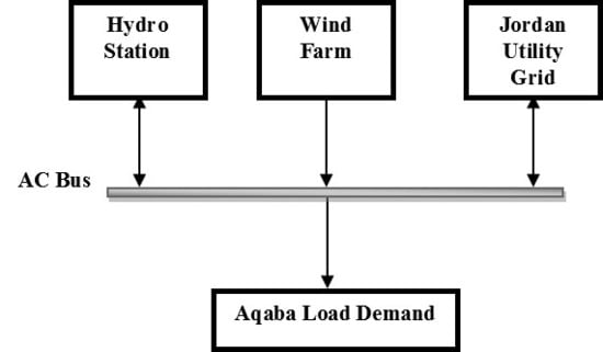
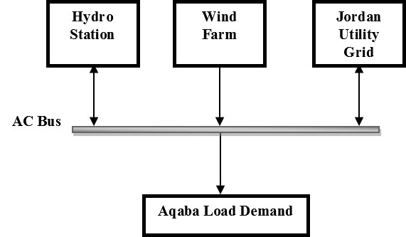
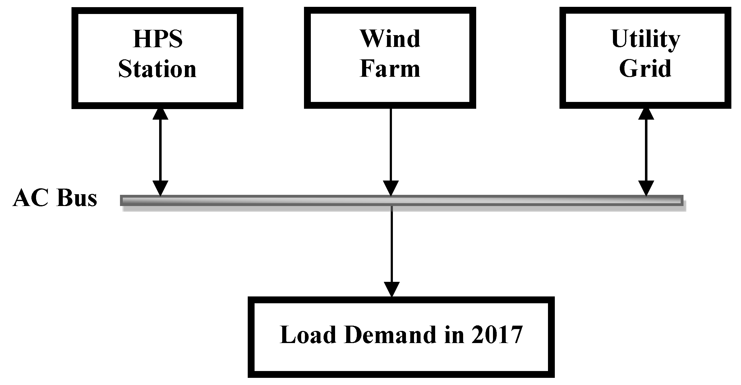
This paper discusses the combination of a wind and hydropower system (See Figure 1), which is integrated with the distribution grid in the country of Jordan, as a case study in an oil-importing country.

The location was the same as one investigated in [12], where an on-grid wind power system was studied in Aqaba, Jordan. However, in this paper, an on-grid wind farm combined with a PHS station was investigated. Therefore, some data are the same, while others are updated for this more up-to-date study. The location was considered to be geographically suitable to construct a PHS station.

Artificial intelligence techniques (GA, SA, and PS) provided by the Matlab optimization toolbox were used to find the optimal solution of the objective function (COE_PS). Then, based on the best fitness, many indicating corresponding functions were computed, such as the wind and hydro fraction (WH_f), grid purchases, the footprint of the renewables, and carbon dioxide emissions (E_CO2). This procedure aimed to help design engineers replicate the same criteria to find optimal solutions for other system configurations to be adopted based on these technical studies and negotiations between electric utilities and investors. Economic, technical, and environmental feasibility impacts were also studied.

2.1. PHS Station Data

The information that was specified for the pumped hydro storage plant to be accurately modeled is shown in

Table 1. Values of parameters used for the pumped hydro storage (PHS) station.

Parameter	Unit	Value
Lifetime	Years	50 [16]
Usable state of charge [1]	%	85
Roundtrip efficiency (ζ)	%	85 [17]
Capital cost	$/kW	1651.04
Operation and maintenance cost (OMC)	(%/Year of capital cost (CC))	1.5
Gross head	m	50
Mean water depth	m	15

. First, the roundtrip efficiency referred to the ratio of the energy out to the energy in over a period of time [13]. It is difficult to separately measure the charging and discharging energies, therefore, manufacturers usually determine the round-trip efficiency and consider it to be the charging efficiency by assuming 100% discharging efficiency. Many authors have discussed this issue in the case of battery systems. Thus, the charging efficiency was set to be equal to the round-trip efficiency, and the discharging efficiency was assumed be in agreement in [14,15].

Second, the usable state of charge (SOC) [1] referred to the ratio of the usable energy that was taken to the total energy of the PHS. In other words, the usable SOC was the energy left in the upper reservoir compared with the amount of energy in a full reservoir. This gave an indication into how long the PHS station could provide energy before a refill. In this study, it was assumed that a minimum stored energy should remain, and this value was the complement of the usable SOC. The usable SOC was assumed to be the same as the round-trip efficiency. Third, an initial PHS stored energy in the upper reservoir was assumed [18]. The aforementioned parameters helped to determine the PHS power generation capacity in kW, which could be used to supply the load as needed. This capacity value was sized using the GA, SA, and PS of the Matlab optimization toolbox. The capital cost of the PHS had an average value of 1651.04 $/kW [16]. The operation and maintenance costs (OMC) were taken as percentages of the capital cost (CC) [16]. Table 1 shows the values that were assumed and considered for the PHS plant. These plant data were used to compute the hourly energy generated. There was an approximate ratio of ten between the rated power (in kW) and energy (in kWh) of the PHS station, as stated in [19].

2.2. Wind Speed and Probability Distribution Function

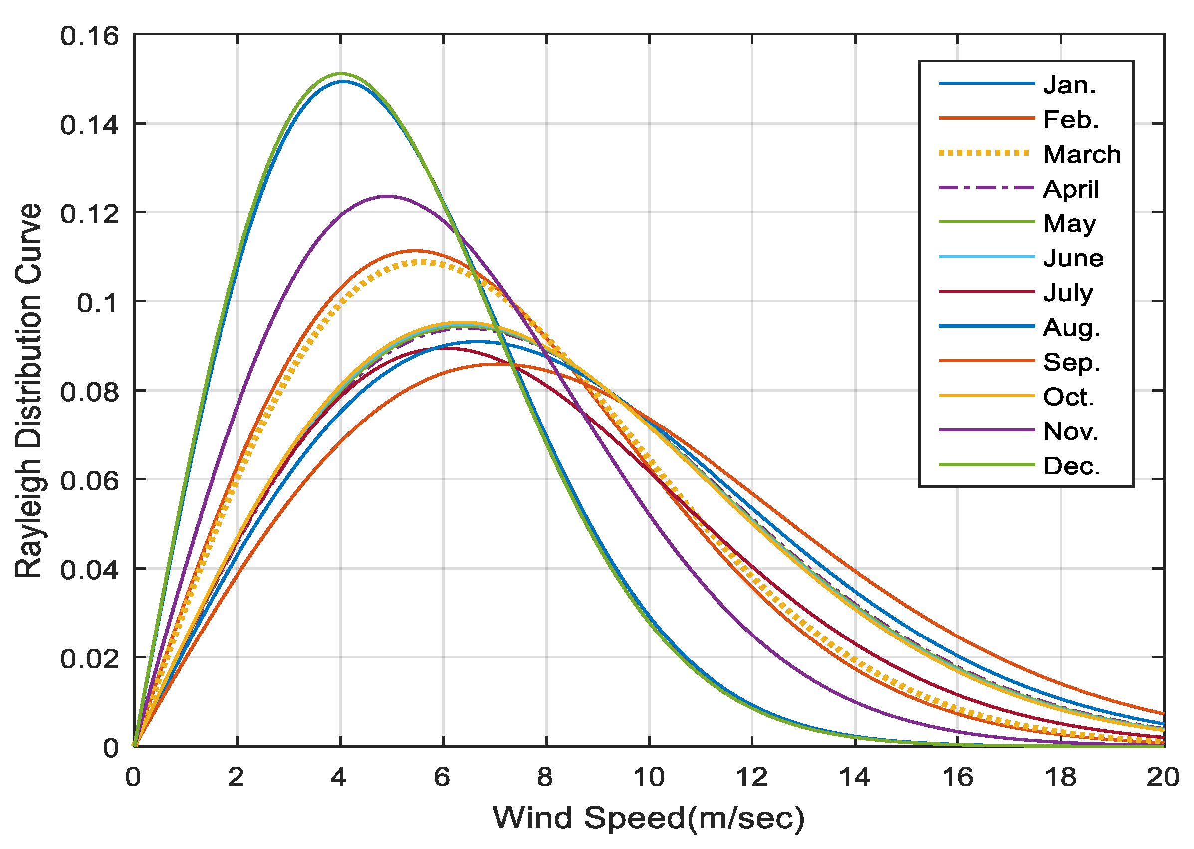
Wind speed can change rapidly in any region. Its variation depends on several factors, such as the surface and the local weather. Appropriate predictions of wind speed in a specific area are necessary for wind power and energy estimations in that area. One of the models for characterizing the wind power is a cubic function of the wind speed. Therefore, a small error in the prediction of wind speed leads to huge variations in the wind energy estimation. Various methods are used to study the characteristics of wind speed. Weibull and Rayleigh distributions are the most preferred methods, as they are flexible and easy in terms of parameter determination.

The focus in this paper was on the Rayleigh distribution, which is a special form of the Weibull distribution with a shape factor that is always equal to two. In the Rayleigh distribution, the mean wind speed is sufficient to determine the wind characteristics. The Rayleigh distribution function (f_R(v)) is given by Equation (1) [20,21].

$$f_R\left(v\right)=\left(\frac{\pi }{2}\right)\left(\frac{v}{v_a^2}\right)exp-\left[\frac{\pi }{4}{\left(\frac{v}{v_a}\right)}^2\right]$$

(1)

where v_a is the average wind speed in a specific area in (m/s). The wind speed logarithmic law shown in Equation (2) was used to model the variation of wind speed due to the difference in height between the anemometers of the metrological station and the hub of the proposed wind turbine. In addition, it considered the terrain roughness between two altitudes [12,22].

$$\frac{v}{v_0}=\frac{ln\left(H/z_0\right)}{ln\left(H_0/z_0\right)}$$

(2)

where v₀ is the wind speed corresponding to the height (H₀) and Z₀ is the roughness coefficient. A case study was conducted in Aqaba, which is the free Trade Area in Jordan. The wind speed was measured in a specific location using anemometer installed at 45 m above ground level, in which the output data was taken on a monthly average basis. Then, Rayleigh distribution was used to obtain hourly data, as shown in Figure 2. The roughness factor of the logarithm used for this case was 0.03 to adjust for the wind speed of open terrain areas [22]. Also, the hub height of the proposed wind turbine was 80 m (

Table 2. Manufacturer information of a C96–2.5 MW wind turbine.

Turbine
Manufacturer	USA
Power
Rated power	2.5 MW
Cut-in wind speed	4.0 m/s
Rated wind speed	12.5 m/s
Cut-out wind speed	25.0 m/s
Survival wind speed	70.0 m/s
Rotor
Diameter	96.0 m
Swept area	7238 m2
Number of blades	3
Maximum rotor speed	15.5 U/min
Tip speed	78 m/s
Type	46.7
Material	Fiberglass
Power density	345.4 W/m2
Gearbox
Type	Spur
Stages	2.0
Tower
Hub height	80.0 m
Type	Steel tube
Shape	conical
Corrosion protection	painted

) which was also considered in the logarithm. The wind speed-based Rayleigh distribution function in Aqaba for twelve months is shown in Figure 2.

Other information that was determined for the wind farm to be precisely sized is shown in

Table 3. Lifetime and spacing parameters of the wind farm.

Parameter	Unit	Value
Life-time per unit	Years	20
Row spacing of the farm (RS)	m	384
Column spacing of the farm (CS)	m	672

. The financial input parameters were the same as the ones described in the wind-only investigation [12]. The project lifetime was assumed to be 50 years. Therefore, the wind turbine will be replaced twice, with a cost that was assumed the same as the capital cost.

The geographical area of the wind farm (A_WF) was computed using Equation (3). L and W are the dimensions of the wind farm, which was considered to have a rectangular shape. For the row spacing (RS) and column spacing (CS) values shown in Table 3, Equations (4) and (5) were used to calculate L and W.

$$A_{WF}=L\times W$$

(3)

$$L=C_S\left(N_{col}-1\right)+D_r$$

(4)

$$W=R_S\left(N_{row}-1\right)+D_r$$

(5)

where D_r, N_row, and N_col are the rotor diameter, number of rows, and number of columns, respectively. These helped to compute the maximum and minimum wind areas, i.e., the A_max and A_min. A footprint cap limit of 20,000 Dunam was considered for the on-grid wind hydro energy system.

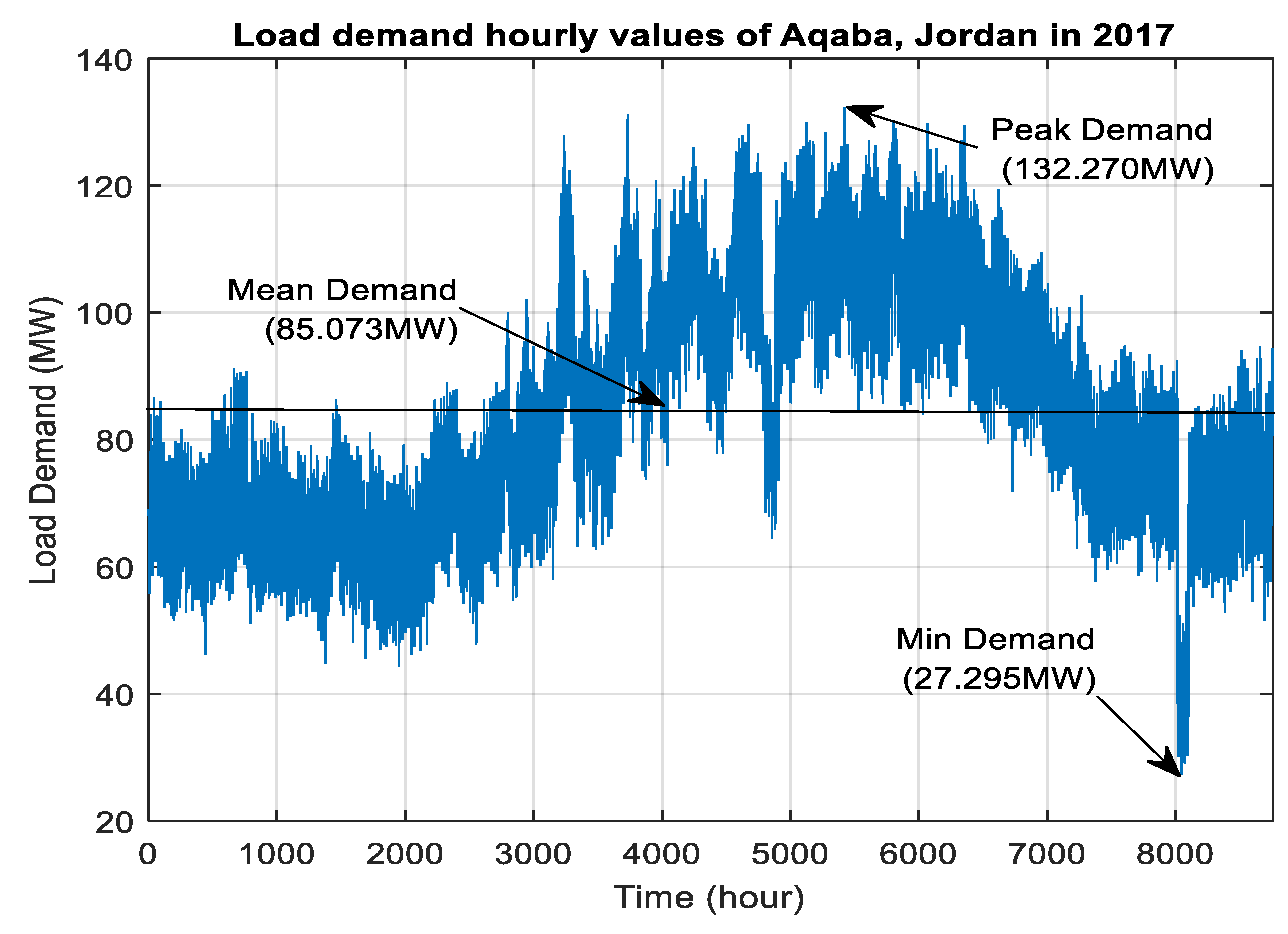
2.3. Load Demand Hourly Data

The load demand hourly values of Aqaba, Jordan in 2017 were prepared after tailoring the supervisory control and data acquisition (SCADA) demand values in 2016 used in [12]. They were obtained from the National Control Center of the National Electric Power Company, Jordan. A percentage growth of 6% for a year is usually used in electric utilities in Jordan to obtain the annual load demand for the following year, therefore, in this paper, the hourly load values in 2017, as shown in Figure 3, were obtained by applying this percentage.

The minimum, maximum, and mean load demand values were 27.295 MW, 132.270 MW, and 85.073 MW, respectively, as shown in Figure 3.

3. Mathematical System Formulation

3.1. Modeling of the Hydro Station

The priority was to satisfy the load from the wind farm. If the wind power was not sufficient, then energy deficit should be covered by the PHS station and, lastly, the energy purchased from the utility grid. The Matlab code had the target of satisfying the entire load. Three cases were considered. First, the load was satisfied by the wind farm, and if there was excess wind power and the reservoir was full, the generation of the hybrid renewable energy system came only from the wind power plant. Second, the load was satisfied by the wind farm, and there was excess wind power and the reservoir was not full. Thus, we computed the excess wind power that could charge the PHS plant by comparing the excess wind power value to the rated capacity of the PHS plant.

Third, when the generation of wind farm was less than what was required by the load demand, we checked the availability of the PHS plant for this power deficit. Moreover, the PHS minimum energy storage capacity was set, which was not exceeded during the discharge.

Once the rated power of the hydro station, P_rated, in kW was optimized, the energy in kWh, W_rated, was estimated based on the assumption made in Section 2.1. Then, the potential energy (in J/m³), W_J, and (in kWh/m³), W_kWh, of water in the upper reservoir were computed using Equation (6) and Equation (7), respectively.

$$W_J={\rho }_{water}gH$$

(6)

$$W_{kWh}=2.78\times {10}^{-7}{W}_J$$

(7)

where ρ_water is the density of water (1000 kg/m³), g is the gravitational acceleration (9.81 m/s²), and H is the actual head of the PHS station [12].

Then, the volume of the water in the upper reservoir (in m³), V_water, was computed using Equation (8). At this point, the area required for the PHS station, A_PHS, was computed using Equation (9) for a given mean depth, D [12]. Furthermore, Equation (10) was used to compute the water flow (F_water) in the pipeline in (m³/s) [23].

$$V_{water}=\frac{E_{rated}}{\eta W_{kWh}}$$

(8)

$$A_{PHS}=\frac{V_{water}}{D}$$

(9)

$$F_{water}=\frac{P_{rated}}{\eta Hg}$$

(10)

3.2. Modeling of the Wind Turbine Power Curve

The wind turbine output power model can be typically presented in two main regions. Region 1 exists between the cut-in speed [1] and the rated wind speed (V_R), while Region 2 exists between V_R and the cut-out wind speed [6], as shown in Figure 4. This shows the ideal model representation of a wind turbine and the corresponding main regions.

To convert the hourly wind speed values, obtained before using Rayleigh distribution, into hourly output wind turbine values, the mathematical model in Equation (11) is used to model Region 1 shown in Figure 4. P_R is the rated power generated by a wind turbine. Further, the corresponding A, B and C parameters are given in Equations (12)–(14) [9,24,25]. This model is different from the ones described in [12]. The output power in Region 1 runs smoothly between V_I and V_R with no protrusions at the cut-in value, as shown in the models described in [12], see Figure 5. This will result in an accurate computation of the output power extracted from the wind farm. This leads to precise computations in the output wind power and energy and thus in the number of units sizing, geographical footprint, economic and environmental indicators.

$$P\left(v\right)=\left\{\begin{array}{cc}{P}_R\left(A+Bv+C{v}^2\right),& V_I\le v\le V_R\\ P_R,& V_R\le v\le V_o\end{array}\right\}$$

(11)

$$A=\frac{1}{{\left(V_I-V_R\right)}^2}\left[V_I\left(V_I+V_R\right)-4V_I{V}_R{\left(\frac{V_I+V_R}{2V_R}\right)}^3\right]$$

(12)

$$B=\frac{1}{{\left(V_I-V_R\right)}^2}\left[4\left(V_I+V_R\right){\left(\frac{V_I+V_R}{2V_R}\right)}^3-\left(3V_I+V_R\right)\right]$$

(13)

$$C=\frac{1}{{\left(V_I-V_R\right)}^2}\left[2-4{\left(\frac{V_I+V_R}{2V_R}\right)}^3\right]$$

(14)

3.3. Objective Function

The objective function in this study was selected to be the cost of energy of the penetrated system (COE_PS) to reflect the price of the energy supplied by the on-grid hybrid wind hydropower system, as designed and sized to cover the load demand shown in Figure 3. It was computed by dividing the system’s cost by the system’s absorbed energy, as shown in Equation (15) [26].

$$CO{E}_{PS}=\frac{Syste{m}^{\prime }s cost}{Syste{m}^{\prime }s absorbed energy}$$

(15)

The system cost was computed by first constructing nominal and discounted cost cash flows for the project lifetime, i.e., 50 years. The nominal cash flow included the capital cost (CC), the replacement cost [22], the operation and maintenance cost (OMC), and the salvage cost (SC). These costs were discounted for the present in the discounted cash flow that represented the total current cost (TCC) of the renewable power system. The system cost calculation criteria are described in detail in [26]. The wind farm financial parameters are described in detail in [12]. The cost parameters of the PHS station are given in Table 1. The cost of the energy from the utility grid had the last priority to satisfy the load demand.

Thus, an economic comparison with one hour time steps was done to satisfy the load demand in Figure 3. However, there were priorities built into the design code to satisfy the load demand; the wind farm first, then the PHS plant, and, lastly, the necessity to purchase energy from the grid if the load was still not satisfied. Moreover, the number of wind turbines (WTs) was computed based on the rated power, as shown Figure 5.

3.4. Indicators of the Objective Function

There are technical, economic, and environmental indicators that were computed based on the optimal value of the COE_PS. These included the wind and hydro fraction (WH_f), as shown in Equation (16), and carbon dioxide emissions (E_CO2).

$$W{H}_f=\frac{Renewable generation}{Syste{m}^{\prime }s absorbed energy}$$

(16)

The E_CO2 was computed by summing up the hourly multiplied grid energy purchases with a grid emission factor of 583.866667 gCO₂/Wh.

4. Optimization Toolbox of Matlab

The optimization toolbox in Matlab is a collection of functions that implement Matlab’s numerical capability and computing environment. This toolbox provides functions to find parameters which minimize or maximize objectives to satisfy specific constraints. Therefore, the optimal solutions of continuous and discrete problems can be obtained, tradeoff analyses can be achieved, and optimization design tasks can be performed using this toolbox. In addition, parameter estimations and tuning can be done using this toolbox. Moreover, solvers for linear programming (LP), quadratic programming, nonlinear programming (NLP), constrained linear least squares, nonlinear least squares, and nonlinear equations are included in this optimization tool box [27]. In this paper, the genetic algorithm (GA), simulated annealing (SA), and pattern search (PS) optimization methods were used from the Matlab toolbox.

GA, which is a search technique based on a principle of biological genetics and natural selection, allows a composition of many individuals to evolve under specified selection rules to a state that maximizes fitness under a specific objective function.

As a Matlab tool, GA is a powerful tool capable of providing robust approximation for systems that may be subject to uncertainties [28,29]. Its research mechanism consists of the use of candidate solutions represented in a binary form, called chromosomes. Several genetic operators, such as crossover, mutation, and inversion, are used to adapt and fit the generated population of chromosomes in each research step [29].

The flow of the genetic algorithm can be summarized by the following steps [30].

• Create initial population (usually a randomly generated string);
• Evaluate all the individuals (apply some function or formula to the individuals);
• Select a new population from the old population based on the fitness of the individuals and the required objective function;
• Apply some genetic operators (mutation, crossover, and inversion) to the population members to create new individuals;
• Evaluate the newly created individuals based on the required objective function.

Repeat the last three steps until the stopping criteria has been satisfied, where a certain fixed number of generations is obtained.

In summary, the GA toolbox has four main modules: The optimization problem definition module, the variables setting module, the generation of the initial population module, and the evolution module. These modules interact with each other by exchanging information that enables the operation of the algorithm. Before running the optimization algorithm, it is necessary to characterize the optimization problem. Then, the type and the representation of the variables used by the algorithm must be defined. GA works directly with real variables or with codified variables. Thus, depending on the type of variable defined by the problem and the type of representation used by the GA, there is a necessity for coding/decoding to pass from the actual workspace to the GA workspace.

Moreover, pattern search (PS), i.e., direct search or derivative-free search, is one of the Matlab optimization methods used to optimize functions that are not continuous or differentiable. Optimization attempts to find the best-match solution with the lowest error value in a multidimensional analysis space of possibilities [27]. Furthermore, simulated annealing (SA) is a Matlab toolbox method used to solve unconstrained and constrained optimization problems [31,32]. The models of this method simulate the heating process of the materials. At each iteration step of the simulated annealing algorithm, a new point is randomly generated. The distance of the new point from the current point is based on a probability distribution with a scale proportional to the temperature. An annealing schedule is selected to systematically decrease the temperature as the algorithm proceeds. As the temperature decreases, the algorithm extends its search to finally reach an optimal solution. The SA algorithm consists of two main options, namely, “AcceptanceFcn” and “TemperatureFcn”. The first option accepts the worst case in order to achieve a global solution for the desired problem. The second option selects the suitable algorithm uses to update the temperature. Two stopping criteria are used for the SA algorithm, which are function tolerance and maximum iterations. In the first criterion, the algorithm runs until the average change in value of the objective function is less than the value of tolerance. In the second criterion, the maximum number of iterations can be determined [27].

5. Results and Discussion

Every component shown in Figure 1 was modeled and coded in Matlab along with the objective function of the cost of energy of penetrated system (COE_PS) and the rest of the corresponding indicators.

Table 4. Detailed results of the optimized system using genetic algorithm (GA), simulated annealing (SA), and pattern search (PS) algorithms.

Parameter	Value (GA)	Value (SA)	Value (PS)
COEPS ($/kWh)	0.0955388	0.0967582	0.0974391
ECO2 (kt/year)	198.9044	204.5988	207.5809
COERenewables ($/kWh)	0.0631	0.0637	0.0641
Number of WTs	47	45	44
Amax (m2)	9,676,800	7,142,400	8,506,368
Amax (Dunam)	9676.800	7142.400	8506.368
Amin (m2)	6,856,704	6,561,792	6,266,880
Amin (Dunam)	6856.704	6561.762	6266.880
Total cost (M$)	441.3	426.37	419.44
WHf (%)	56.1427	54.3791	53.4641
Grid purchases cost (M$)	45.649	46.956	47.641
Grid energy purchases (GWh)	340.67	350.42	355.53
Prated (PHS) (kW)	18,118.5	19,226.37	20,039.45
Erated (PHS) (kWh)	181,185	192,263.7	200,394.5
WJ (J/m3)	4.905 × 105
WkWh (kWh/m3)	0.136359
Vwater (m3)	1.56322 × 106	1.65880 × 106	1.72895 × 106
APHS (in m2)	104,214.902	110,586.803	115,263.501
APHS (in Dunam)	104.2149	110.5868	115.2635
Fwater (m3/s)	43.457	46.115	48.065

shows the results obtained using the GA, SA, and PS solvers. Also, many data corresponding to the optimal value of the COE_PS are included in Table 4. The three aforementioned solvers of the Matlab optimization toolbox were selected to solve the problem described in this paper. The SA and PS solvers provided solutions that were 1.27634% and 1.98903% higher than the GA solution, respectively. Therefore, the GA solution was found to be feasible compared with the other solutions.

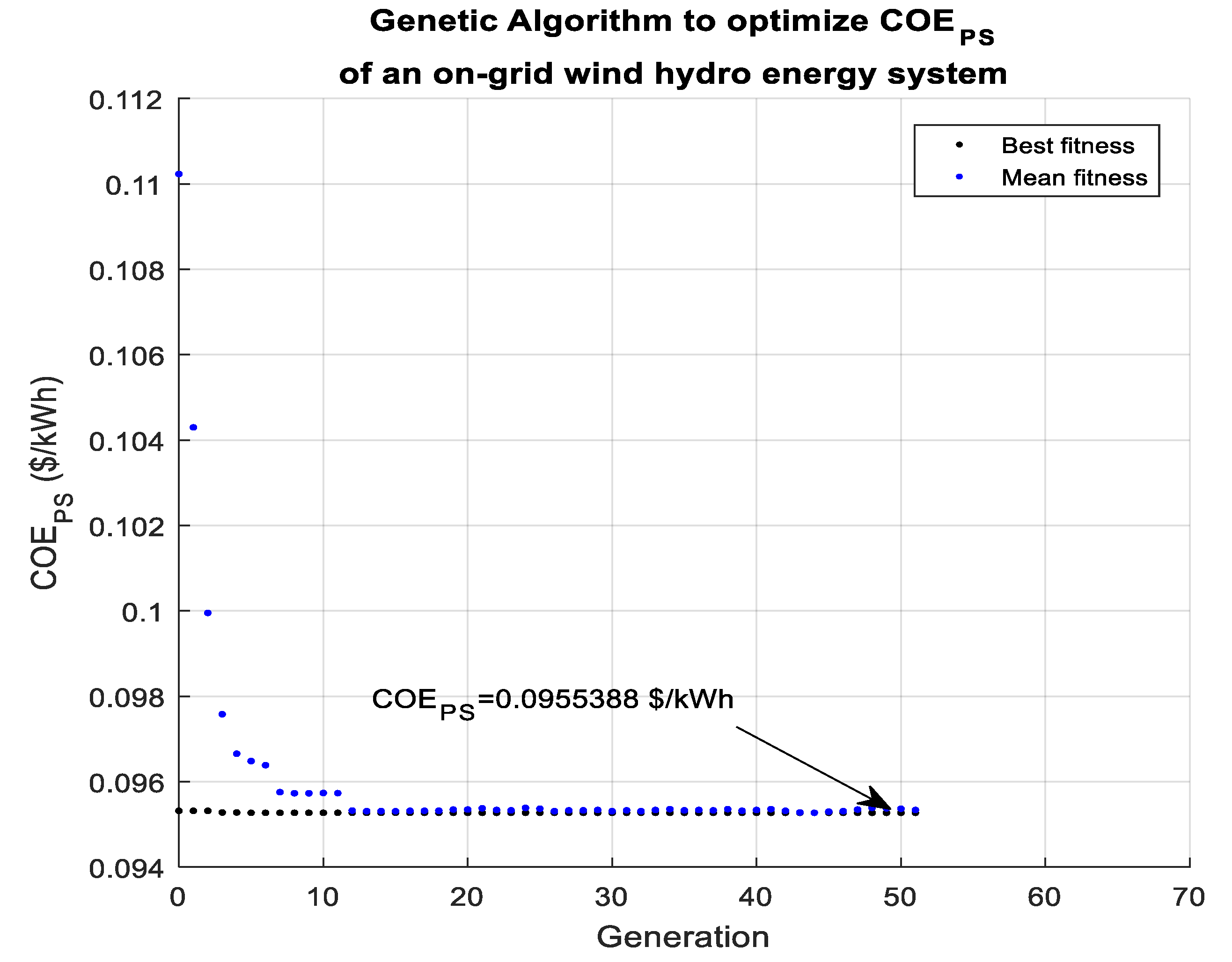
The GA solution of 0.0955388 $/kWh was economically feasible compared with the SA and PS COE_PS values. The optimal value of the COE_PS, which was found using the GA, is shown in Figure 6. This value was 28.7% less than the energy bought from the conventional electric network, which is an excellent indication for the economic feasibility of this suggested configuration.

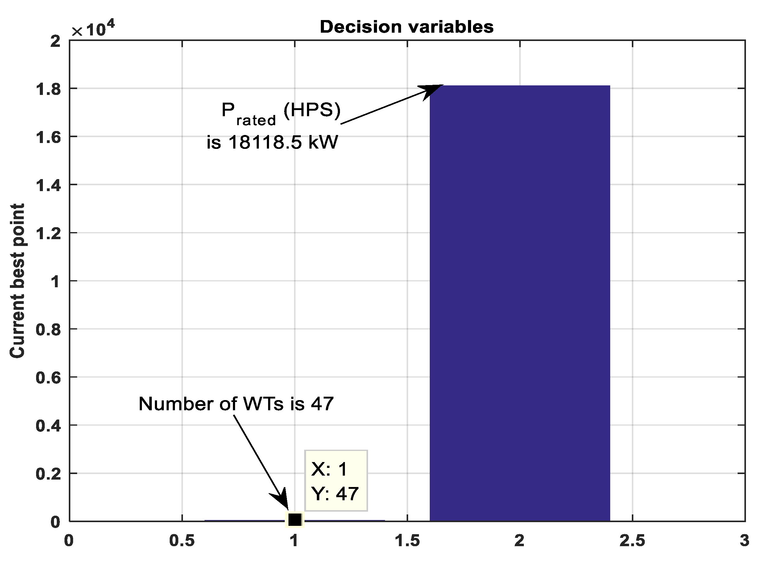
Further, Figure 7 shows the current best point for the two decision variables found at the optimal value of the objective function.

Note that the area of the wind farm was assumed to be rectangular and was therefore computed by incrementing the odd optimal number by one. Furthermore, the E_CO2 in the suggested location was 634.645 kt/year [12], therefore, the emissions were mitigated by 68.66%, assuming that the renewable configuration in Figure 1 was adopted. Also, the geographical area of renewable plants (A_Renewables) was increased. However, only 48.91% of the geographical area limit was used to install the designed hydro-wind energy system. Thus, the rest of the area (51.09%) could be used in the future as load demand and the system size grow.

The discounted payback period (DPP) is frequently used in renewable energy studies to find the length of time needed to retrieve the initial investment [33,34,35]. This was done in this paper by building the cumulative cash flow (CCF), as shown in

Table 5. Calculation of the discounted payback period.

Year (N)	PVF	CF (M$)	CFdiscounted (M$)	CCF (M$)
0	1.000	−441.300	−441.300	−441.300
1	0.944	58.483	55.234	−386.066
2	0.892	58.483	52.165	−333.901
3	0.842	58.483	49.267	−284.633
4	0.796	58.483	46.530	−238.103
5	0.751	58.483	43.945	−194.158
6	0.710	58.483	41.504	−152.654
7	0.670	58.483	39.198	−113.456
8	0.633	58.483	37.020	−76.436
9	0.598	58.483	34.964	−41.472
10	0.565	58.483	33.021	−8.451
11	0.533	58.483	31.187	22.736
12	0.504	58.483	29.454	52.190
13	0.476	58.483	27.818	80.008
14	0.449	58.483	26.272	106.280
15	0.424	58.483	24.813	131.093
DPP (Years)		10.27096862

. Note that the present value factor (PVF), cash flow (CF), and the corresponding discounted cost values (CF_discounted) were calculated. The CF in Table 5 included the total cost found before in Table 4 using GA, and the energy savings of the renewable energy system. These energy savings were computed by multiplying the yearly renewable generation (436.438 GWh) by the energy purchased price of electric utilities in Jordan. Afterward, the CCF values were computed by cumulatively adding the discounted cost values. Then, the time to get back the total cost value was calculated using Equation (17). Note that Table 5 shows only 15 years of the 50-year project life-time, because the aim was to obtain a positive cost value from the CCF, which was held at the 11th year. This was just before the time when the total cost was retrieved. Table 5 shows that the DPP was computed to be around 10.271 years (10 years, 3 months, and 7 days).

$$DPP=n_l+\frac{\left|CCF \left(n_l\right)\right|}{C{F}_{discounted}\left(n_l+1\right)}$$

(17)

where n_l is the year number at the last negative cost value of the CCF.

The study performed in this paper, after adding the hydro storage system, was compared to a previously studied scenario in [12] for a wind-only system connected to the utility grid at the same location.

Table 6. On-grid wind farm with/without PHS comparison.

Parameter	Percentage Increase (+) or Decrease (−) in %
COEPS	−12.26
ECO2	−24.69
COERenewables	−1.52
Number of WTs	+104.35
ARenewables (max)	+71.14
ARenewables (min)	+21.79
Total cost	+110.83
WHf	+56.64
Grid purchases cost	−24.69
Grid energy purchases	−24.68

shows the percentage increase/decrease for the parameters computed in Table 4. For the wind–hydro on-grid system, the COE_PS and the grid purchases were reduced by 16.93% and 24.68%, respectively, showing the importance of the storage system for wind power that fluctuates naturally. These cost and emissions reductions are significant, especially for non-oil producing countries, such as Jordan, which imports around 96% of its energy needs as oil and natural gas. The carbon emissions reduction was improved compared with the wind-only system. Furthermore, renewable penetration increased by 56.64% as a result of adding the PHS system, resulting in a more environmentally friendly power system.

6. Conclusions

In this paper, every component shown in Figure 1 was modeled and coded in Matlab along with the objective function (COE_PS). A wind–hydro grid connected power system was proposed as an adjunct to an existing power grid. This was mathematically modeled and then coded in Matlab. The GA of the Matlab optimization toolbox was used to find the optimal feasible value of the COE_PS, which was 0.0955388 $/kWh. This was 28.7% less than the conventional energy from the power grid. The discounted payback period was 10 years, 3 months, and 7 days. Furthermore, carbon emissions were reduced by 68.66% compared with experimentally estimated data. As a result, the grid energy purchases were also reduced. Specifically, comparing the system described in this study with the formerly studied on-grid wind-only system showed that the COE_PS, E_CO2, COE_Renewables, and grid energy purchases were reduced by 12.26%, 24.69%, 1.52%, and 24.68%, respectively. These are very promising results, especially for oil-importing countries, such as Jordan, where imported energy is a significant financial burden to the economy. The proposed wind power system with hydro storage is recommendable for its clean and economical features, compared with the conventional fossil-fueled grid or wind-only on-grid renewable configurations.

Finally, this paper is a case study to demonstrate the important point of local solutions to the global problem of global warming. The paper is necessarily limited to the specific data and assumptions of the local case study. Future work will include applying the above principle and the methodology of this paper to many other local engineering boundary conditions.