Article

Numerical Study of Nacelle Wind Speed Characteristics of a Horizontal Axis Wind Turbine under Time-Varying Flow

1
Key Laboratory of Condition Monitoring and Control for Power Plant Equipment, Ministry of Education, North China Electric Power University, Beijing 102206, China
2
China Resources Power Technology Research Institute Co., Ltd., Shenzhen 518026, Guangdong, China
3
Department of Aerospace Engineering, Iowa State University, Ames, IA 50011, USA
*
Author to whom correspondence should be addressed.
Energies 2019, 12(20), 3993; https://doi.org/10.3390/en12203993
Submission received: 25 September 2019 / Revised: 16 October 2019 / Accepted: 17 October 2019 / Published: 20 October 2019
(This article belongs to the Section A3: Wind, Wave and Tidal Energy)

Abstract

:
Nacelle wind speed transfer function (NTF) is usually used for power prediction and operational control of a horizontal axis wind turbine. Nacelle wind speed exhibits high instability as it is influenced by both incoming flow and near wake of a wind turbine rotor. Enhanced understanding of the nacelle wind speed characteristics is critical for improving the accuracy of NTF. This paper presents Reynolds-averaged Navier–Stokes (RANS) simulation results obtained for a multi-megawatt wind turbine under both stable and dynamic incoming flows. The dynamic inlet wind speed varies in the form of simplified sinusoidal and superposed sinusoidal functions. The simulation results are analyzed in time and frequency domains. For a stable inlet flow, the variation of nacelle wind speed is mainly influenced by the blade rotation. The influence of wake flow shows high frequency characteristics. The results with stable inlet flow show that the reduction of the nacelle wind speed with respect to the inlet wind speed is overestimated for low wind speed condition, and underestimated for high wind speed condition. Under time-varing inflow conditions, for the time scale and fluctuation amplitude subject to the International Electrotechnical Commission (IEC) standard, the nacelle wind speed is mainly influenced by the dynamic inflow. The variation of inflow can be recovered by choosing a suitable low pass filter. The work in this paper demonstrates the potential for building accurate NTF based on Computational Fluid Dynamic (CFD) simulations and signal analysis.

1. Introduction

The use of wind power has been developing rapidly all over the world during the past few decades. The aerodynamic performance of wind turbines is a key element in wind power production. Power prediction and operation monitoring of wind turbines require accurate prediction of wind speed in front of wind turbines. Usually, met mast or ground LIDAR is used to measure the wind speed. However, the number of met masts in a wind farm is limited due to high installation costs. Normally, only one or two met masts are built for one wind farm, which is not enough for accurate wind prediction of every wind turbine present in the wind farm. Nacelle LIDAR has been proposed for power measurement in recent years [1,2]. This technology is still under development and not widely applied. In practical engineering scenarios, an anemometer mounted on the wind turbine nacelle, i.e., a nacelle anemometer, is still the most often used instrument for wind prediction as it is cheap and easy to setup.
For an upwind horizontal axis wind turbine (HAWT), which at present is the main type of wind turbine in large-scale wind farms, the nacelle anemometer is located downstream of the wind turbine rotor. The flow measured by the anemometer is usually different from the flow in front of the wind turbine due to the disturbance and obstruction caused by blade rotation and nacelle geometry, respectively. Thus, the wind speed measured by the nacelle anemometer has to be adjusted according to the upstream wind speed. In other words, a transfer function between the nacelle wind speed and the incoming wind speed, i.e., a nacelle transfer function (NTF), is needed. At present, the most commonly used adjustment method uses curve fitting of average wind speed based on met mast measurements. According to the International Electrotechnical Commission (IEC) standard 61400-12-2:2013 [3], the NTF can be generated by curve fitting between the averaged wind speeds measured by a met mast and a nacelle anemometer. This method is widely used since it is simple and easy to implement in practical engineering applications. One of its drawback is the self-consistency check criterion of IEC standard 61400-12-2, which is difficult to satisfy. Low quality measurements often result in failure to meet this criterion, which occurs frequently according to Kirshna et al. [4]. Another drawback of this method is that the time scale is usually too large to be used in wind turbine control because the physical correlation between the nacelle wind and the freestream wind cannot be obtained using this data-driven NTF method. Significant challenges still exist in understanding the underlying physics using the available data [5].
The NTF is strongly related to the wake flow of wind turbine, which has been investigated extensively during the past decades. Vermeer et al. [6] presented a detailed review of research carried out on wind turbine wake aerodynamics during the last century. Usually, the wake flow can be divided into near wake region and far wake region. According to Vermeer and Sørensen [6], the former region is the area just behind the rotor, approximately up to one rotor diameter (D). In this region, the influence of rotor geometry, stalled flow, three dimensional (three-dimensional) effects, as well as the tip and root vortices, are significantly high. The far wake region is beyond the near wake, where the effects of these factors are less significant. Far wake has been modeled successfully using wake models, such as Jensen model [7], Larsen model [8], Ainslie model [9], etc., which are usually simple and fast. On the other hand, it is difficult to build simplified models for the near wake, as it is strongly related to the blade aerodynamics. Most of the existing research on near wake focused on the tip and root vortices, as well as the stalled flow. Whale et al. [10] investigated the vortex wake of a two-blade model wind turbine using particle image velocimetry (PIV) measurements and free-wake modeling. The tip vortex pitch is modelled accurately in the simulations. It was found that the helical vortex wake was insensitive to blade chord Reynolds number when the tip speed ratio was kept constant. Massouh and Dovrev [11] also investigated the near wake of a small model wind turbine with three blades using both PIV and hot wire anemometry (HWA) measurements. The results revealed the expansion of tip vortices in a radial direction. The tip vortices are the only vortices that can be observed farther than 2D distance downstream. Micallef et al. [12] investigated the tip vortex of the MEXICO rotor in both axial and yaw cases. The experimental results established the generation mechanisms of the tip vorticity and showed three-dimensional flow behavior under yaw, which was not fully captured by the previously mentioned free-wake vortex models.
Compared to the tip vortices, the root flow did not receive significant research attention due to lower power production in the blade root region. However, the root flow is important as it affects the near wake and nacelle wind speed measurement. Several experiments have been performed to study the root flow in scaled wind turbine models. In Whale’s experiments [10], it was found that the root vortex had the same sign as the tip vortex, and it merged with the tip vortex at an approximate distance of 1.0D behind the rotor plane. As the rotor diameter of the model was small (175 mm), it is possible that the interaction between the tip vortex and root vortex may not be the same for large-scale wind turbines. Ebert and Wood [13,14] performed a series of wind tunnel measurements on the near wake of a model-scale wind turbine. For high tip velocity ratios, the hub vortex became a cylindrical vortex sheet over a short distance downstream. The downstream axial vorticity was supposed to be formed from the circumferential vorticity in the boundary layer upstream of the blades. In experiments presented by Massouh and Dovrev [11], the reversal zone behind the hub was significantly expanded due to the interaction between rotor and the hub boundary layer. There was an increase of circulation near the hub over a smaller range of r, indicating a compact hub vortex. Hu et al. [15,16] investigated the near wake characteristics of wind turbine models in an atmospheric boundary layer using PIV measurements. The evolution of vortex structure in the near wake was correlated to the dynamic load variation of wind turbine. Zhang et al. [17] measured the structure of near wake flow downwind of a model wind turbine in a neutral boundary layer using PIV. It was found that the hubroot vortices were significant within 1.5D distance downstream, and dissipated faster than the tip vortices. Several experiments using PIV measurements to investigate the near wake flow properties were presented in [18,19,20,21]. However, the wind tunnel experiments suffered from scaling issues.
Numerical simulations have been employed to study the near wake flow. In Blade Element Momentum (BEM) methods, a loss factor is added to consider the influence of root vortex. However, the flow in the root region is fully three-dimensional and viscous, which cannot be effectively modelled with the BEM methods. Advanced methods with high credibility, such as computational fluid dynamic (CFD), are needed. Sanderse et al. [22] reviewed the state-of-the-art numerical calculation of wind turbine wake aerodynamics. They pointed out that the actuator approach seems more suitable for the far wake modelling. For the near wake, more validations of the actuator methods to model the effect of the blade geometry are required. Porté-Agel et al. [23,24] investigated the wake flow after a miniature wind turbine in a neutral turbulent boundary-layer, using large-eddy simulation (LES) coupled with actuator–disk (AD) model with rotation (ADM-R) and without rotation (ADM-NR). The ADM-R results showed better agreement with the experimental data than the ADM-NR results in the near-wake region. Lignarolo et al. [25] validated the AD method using wind tunnel experiments. It was found that the AD type methods often failed at modeling the effects of flow turbulence due to the absence of blade tip vortices and their breakdown. Sorensen et al. [26] simulated the flow around the MEXICO wind turbine using Reynolds-averaged Navier–Stokes (RANS) simulations. Excellent agreement between computational results and experimental data for three velocity components were obtained within one rotor diameter downstream of the rotor. Nacelle was not modelled, which was found to have substantial influence under yaw conditions. O’Brien et al. [27] compared the performance of three turbulence models using simulations of the near wake of a three-bladed HAWT model. The wind turbine was modeled with full geometry. The highest velocity deficit was consistently located behind the nacelle and tower which introduced considerable recirculating flow into the near wake.
Most of the above-mentioned literature focused on flow structure of the tip and root vortices in near wake. Only a few papers investigated the flow around the nacelle that is very close to the rotor. Masson and Ameur studied the nacelle flow. Masson and Smaïli [28] studied the turbulent flow around a wind turbine nacelle using RANS simulations. The AD method was used to approximately model the wind turbine rotor. It was shown that the numerical method was useful for placing nacelle anemometers to reduce the influence of high spatial variation and fluctuations in atmospheric turbulence on the nacelle wind speed. Ameur et al. [29] investigated the wind-rotor/nacelle interaction using both two-dimensional (two-dimensional) and three-dimensional RANS simulations. The three-dimensional simulation results showed better agreement with the measurement data than the two-dimensional results. Ameur and Masson [30] compared three types of AD methods. The actuator line approach provided the best results compared to the actuator disk considering the NTF curve. As the wind turbine was simulated by an AD type method, and steady simulations were performed, only an average wind speed was obtained. Zahle and Sørensen [31] investigated the nacelle wind speed for a small-scale wind turbine using RANS simulations. Full geometry of the wind turbine rotor was modeled. The authors observed that, at low wind speeds, steady simulations overestimated the wind speed reduction on the nacelle compared to the unsteady simulations. At high wind speeds, the situation was reversed. The inflow velocity was constant during the simulations.
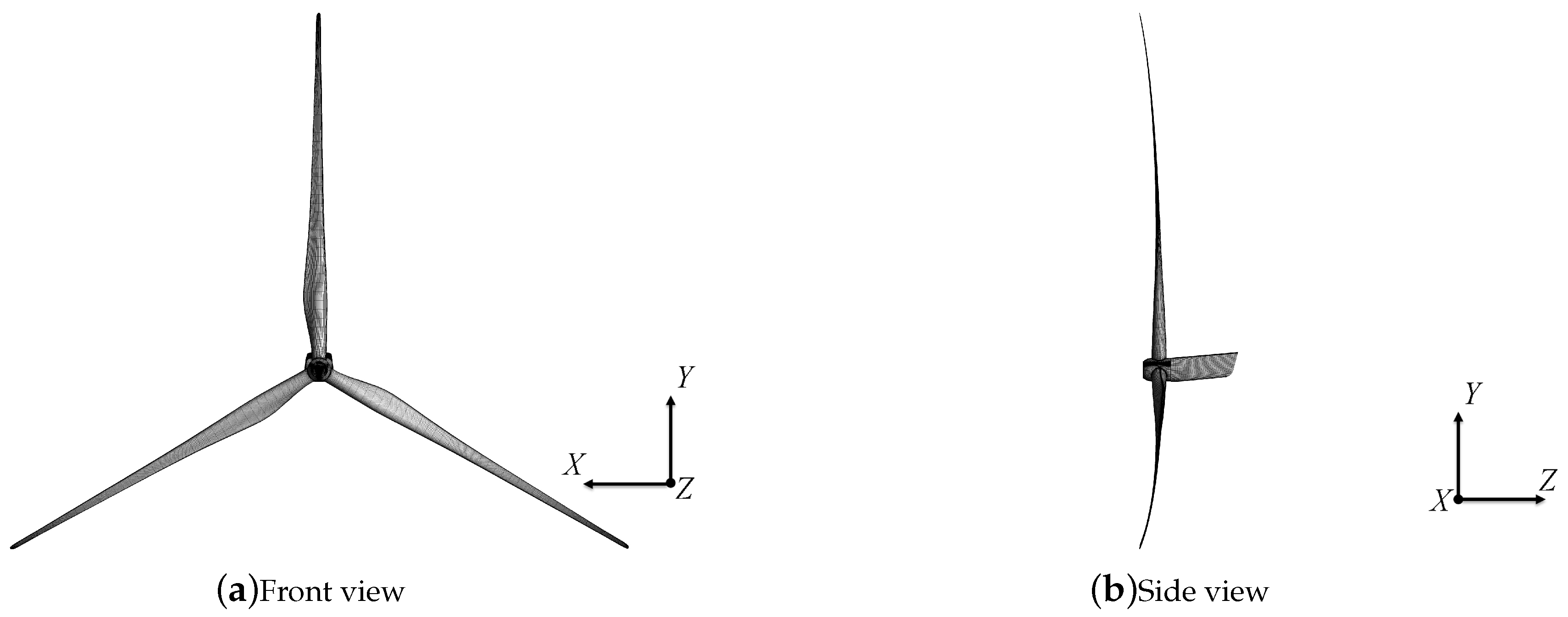
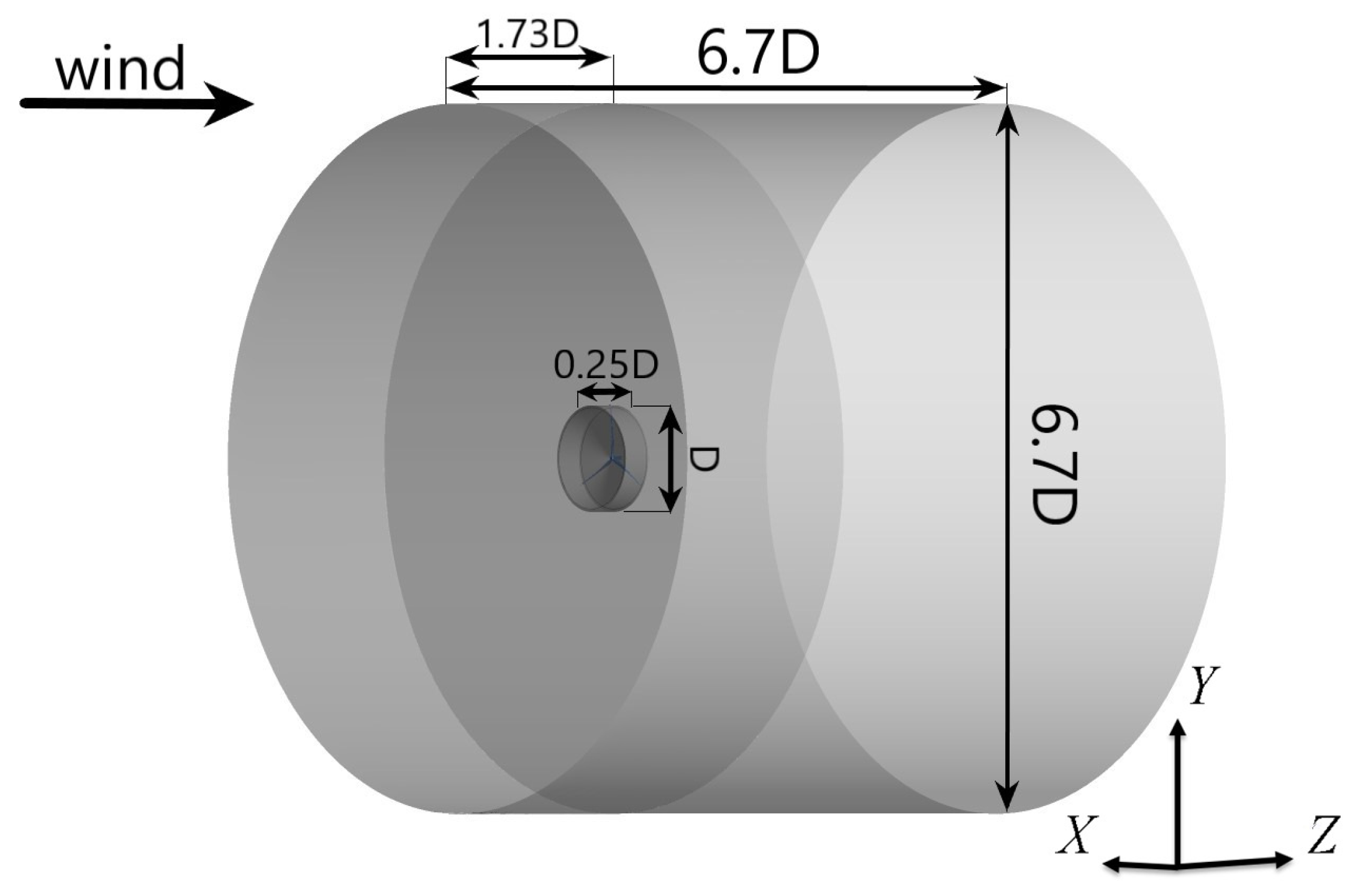
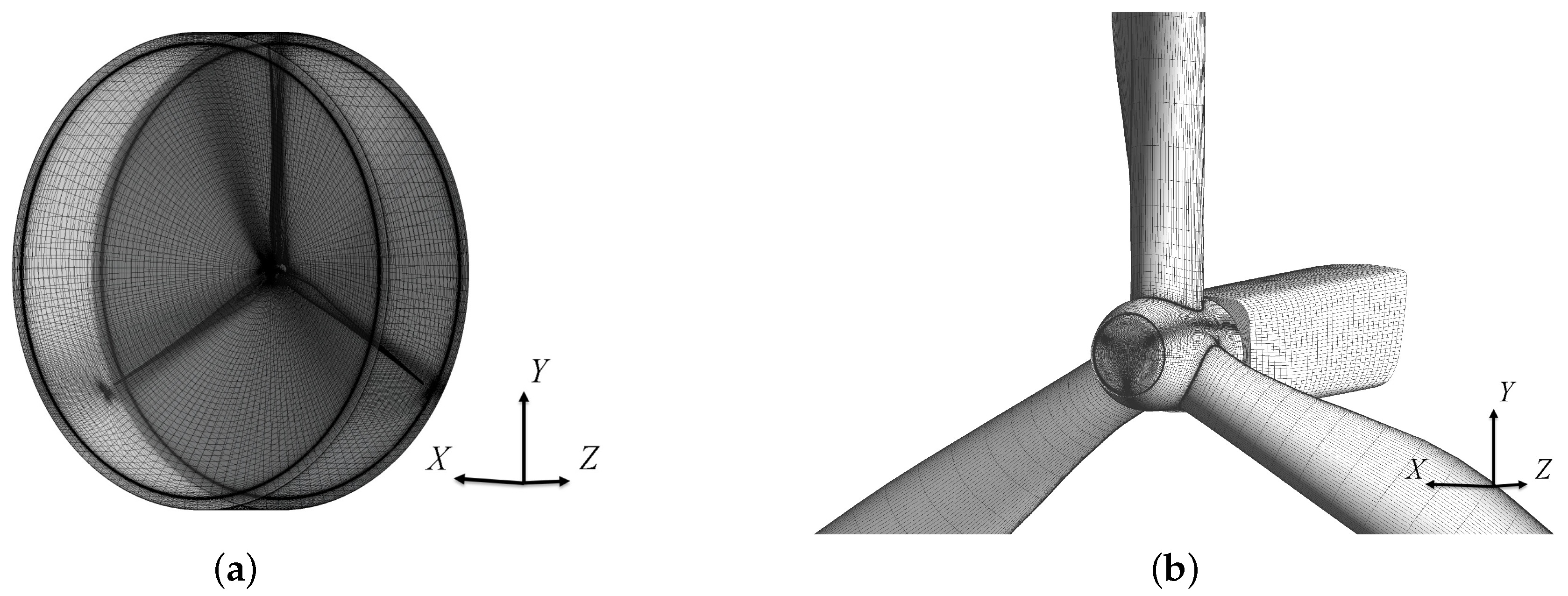
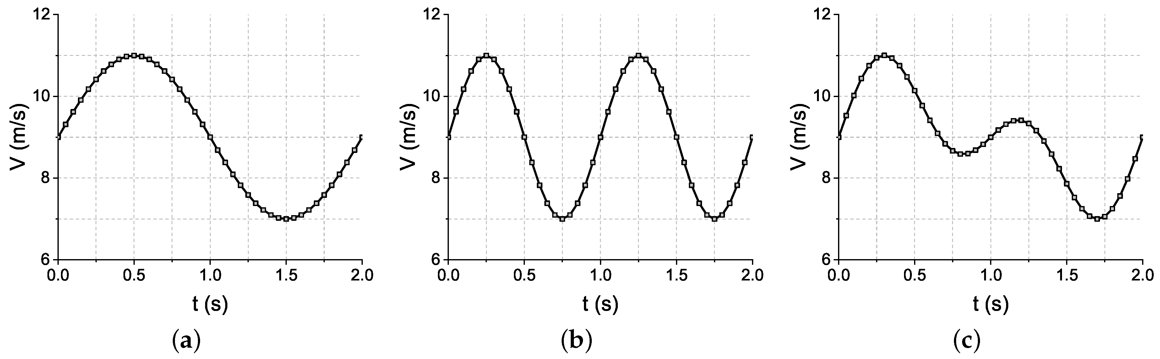
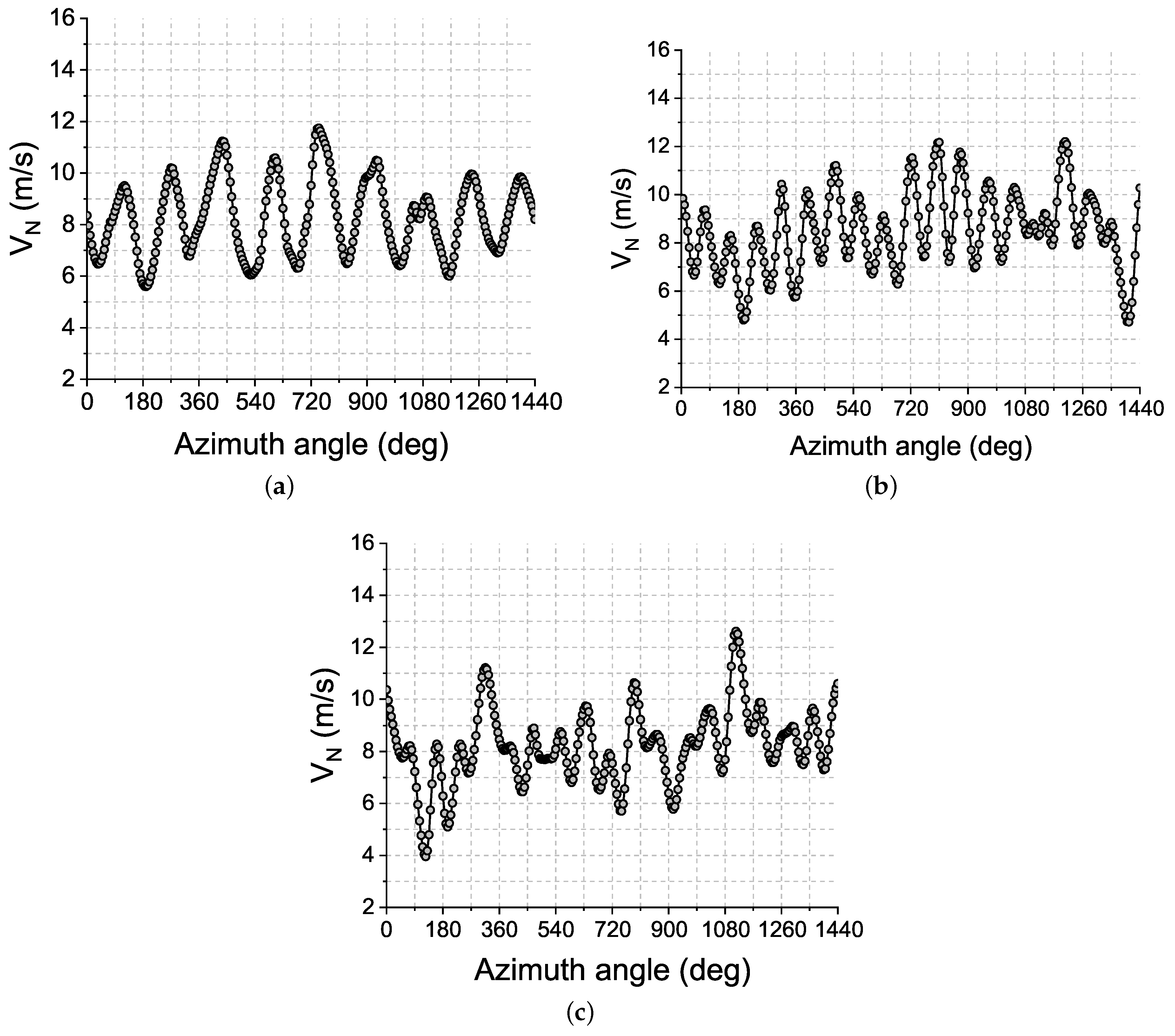
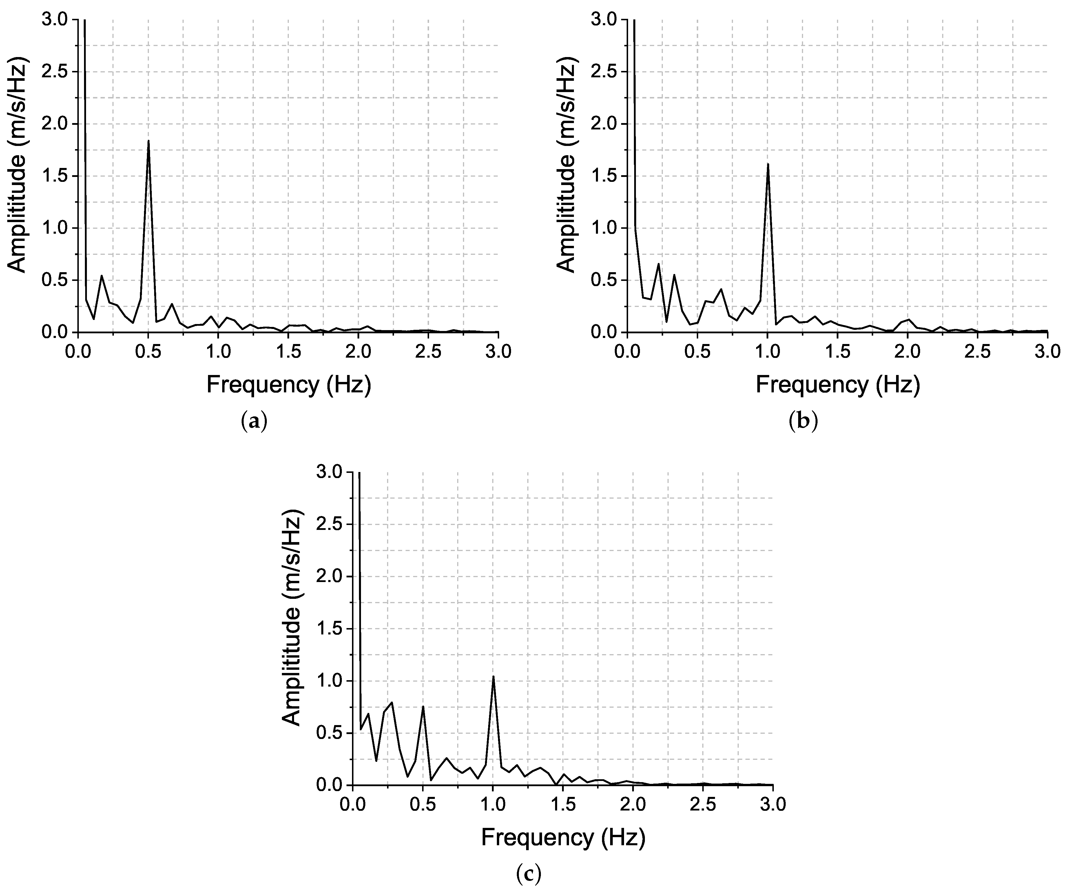
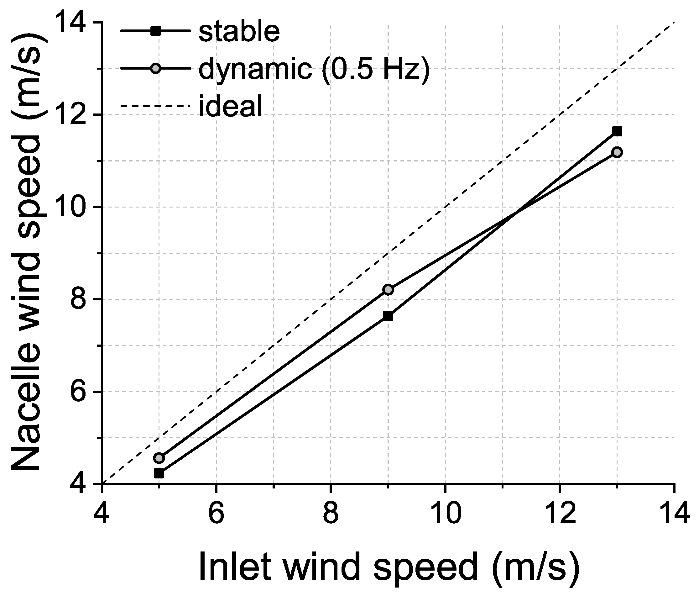
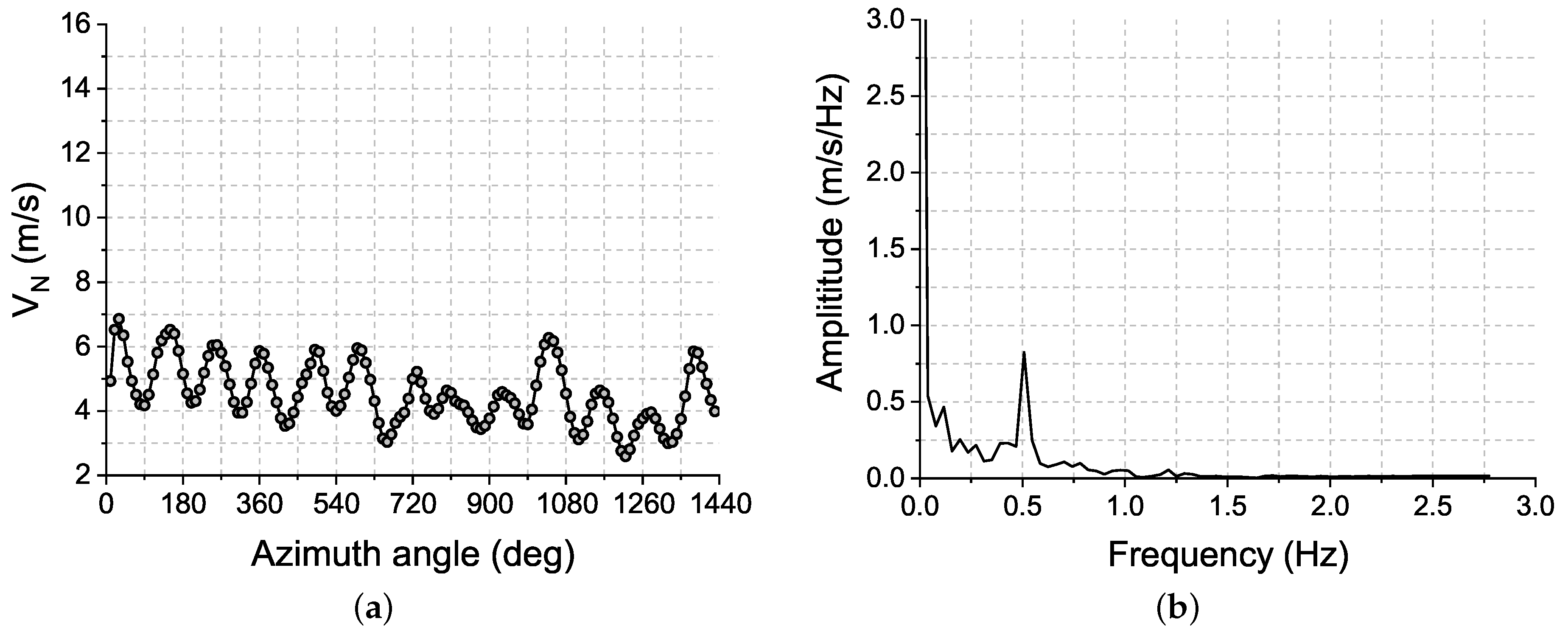
Based on the literature survey, it can be concluded that a comprehensive analysis of the characteristics of the nacelle wind speed, especially for unstable inflow, is needed. Enhanced understanding of the time-varying characteristics of nacelle wind speed and correlation with the unsteady inflow are very critical for construction of an accurate NTF. In order to address these points, this paper investigates the flow around the nacelle region of a HAWT using CFD simulations with the rotor geometry fully modeled. Both stable inflow and dynamic inflow varying in the form of simplified functions are investigated. The paper is organized as follows: Section 2 describes the geometry model and computational methods. In 
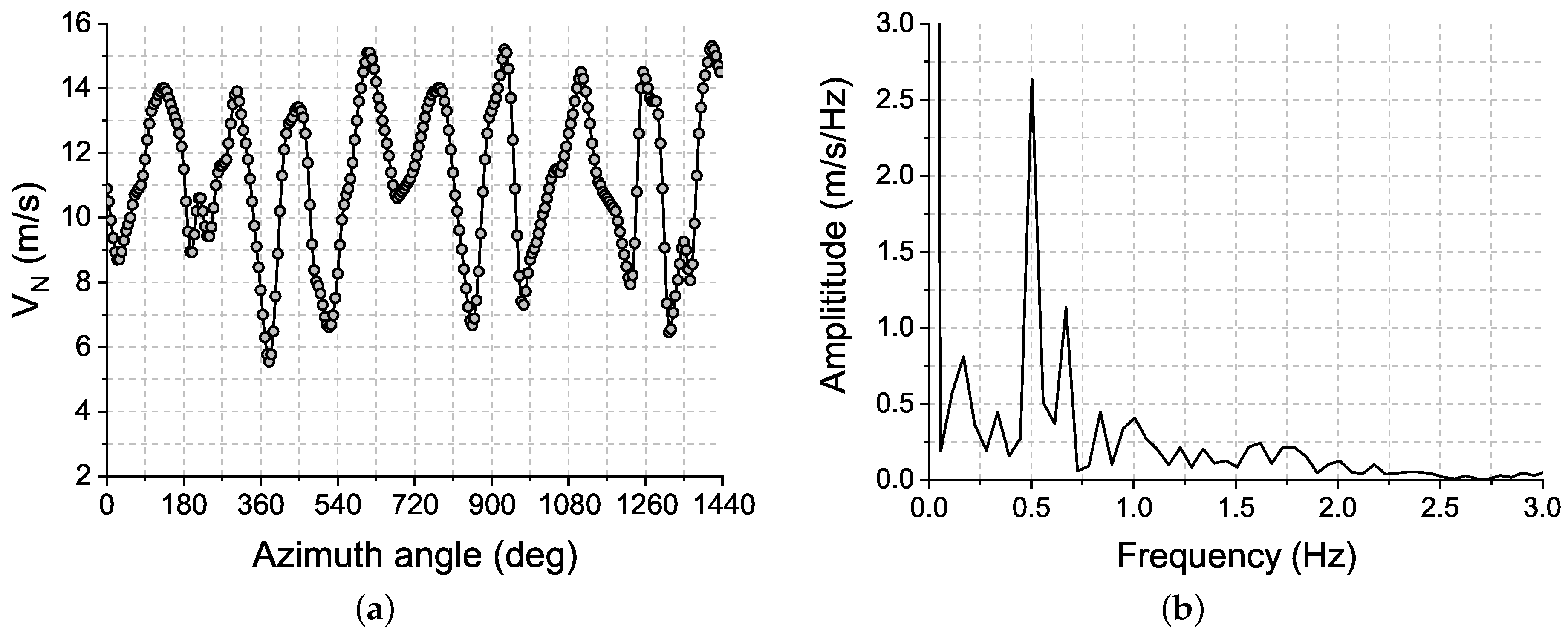
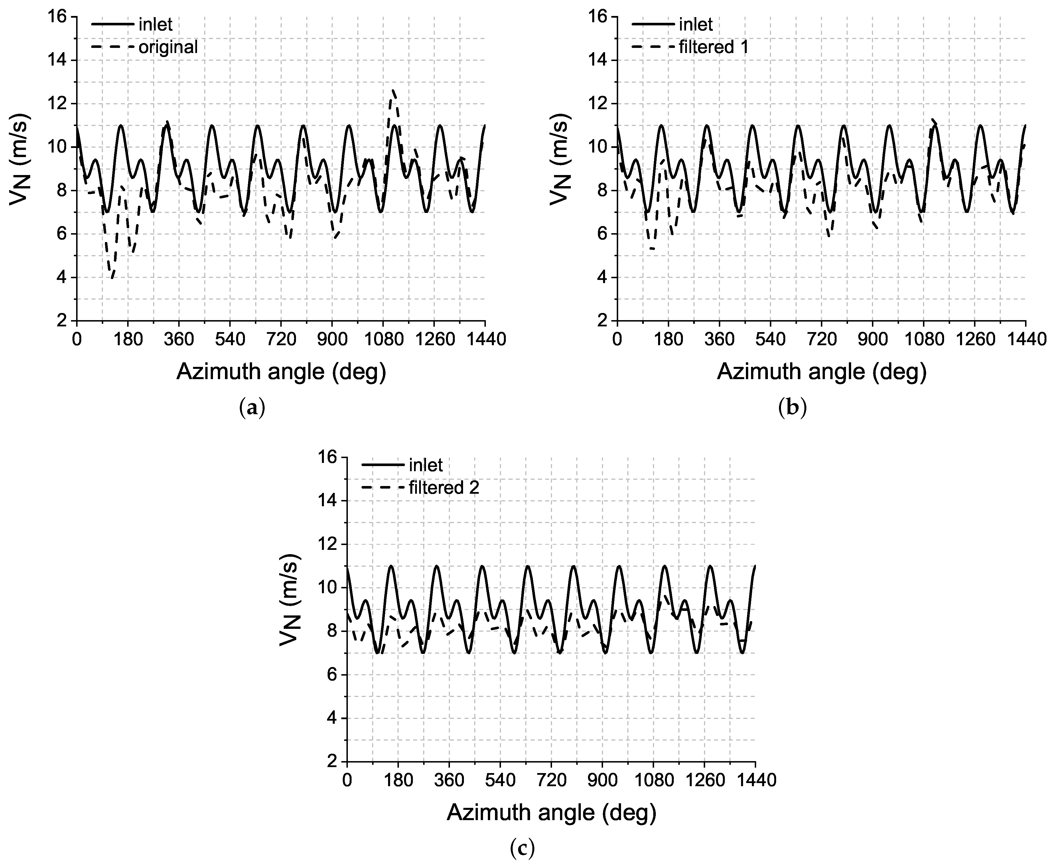
Section 3, the characteristics of nacelle wind speed are analyzed in both time and frequency domains. Section 4 presents the conclusions drawn in this paper.

2. Wind Turbine Model and Numerical Methods

2.1. Wind Turbine Model

A three-bladed horizontal axis wind turbine with a rated capacity of 2 MW is investigated in this paper. The power coefficient at rated wind speed is about 0.45. The thrust force is about 333 kN. A three-dimensional model is generated, which includes the wind turbine rotor, hub, and nacelle. Figure 1 shows the geometric model of the wind turbine. As this paper mainly focuses on the near wake flow on the top of nacelle, the effect of tower can be neglected and, subsequently, the tower is not included in the model. The rotational diameter, D, is 116 m. The hub is a combination of a hemisphere and a cylinder. The maximum diameter of the hub, d, is 3.6 m. The end of hub cylinder is connected with the nacelle, which is close to a cuboid with rounding tail. The length, width and thickness of the nacelle are about 10.8 m, 4.2 m and 3.8 m, respectively. The rotor has an elevation angle of 5°.

2.2. Computational Domain and Boundary Conditions

The computational domain is divided into two subdomains, as illustrated in Figure 2, a rotational domain, and a far-field domain. The former domain is a cylinder with a diameter of 1.05D and a height of 0.25D. The wind turbine blade and hub are located at the center of this domain. The far-field domain is a non-rotating domain, which is also a cylinder having both diameter and height equal to 6.7D. The nacelle is located in the far-field, which is connected with the back surface of the hub. The axes of both domains are consistent with the rotational axis of the wind turbine in the z-direction. The inlet boundary condition is set to the left surface of the far-field domain, which is at a distance of about 1.73D to the rotor. Since only the wind turbine rotor and nacelle are modelled, the wind shear is not considered in this study. The influence of the rotor to the upstream flow is very small. Thus, the inlet distance is long enough, which also can be seen from the results’ validations. The right surface of the far-field domain is set to the outlet boundary condition, which is at a distance of about 4.97D to the rotor. The revolution surface is set to free slip walls, and the blade and hub surfaces are set to no slip walls.

2.3. Computational Mesh

A multi-block full structured mesh is used for computations. The mesh in rotational domain is generated using AutoGrid software from NUMECA Inc. (Belgium). The number of nodes in the grid is 2.52 million, about 840 thousand nodes per blade. The number of nodes in the grid for the far-field domain and nacelle is about 3.10 million. Thus, the total number of nodes in the grid is 5.62 million. The mesh near the blade, hub and nacelle surfaces is refined further. The height of the first cell normal to the surface is 0.2 mm. In most regions, y + < 2 . The maximum y + is around 5. According to the validation case presented in the Fluent manual, the relative difference of transition onset is very small for 1 < y + < 8 [32]. The mesh used in this study generally satisfies the requirement of low Reynolds number turbulence model [33]. The mesh for the wind turbine rotor is illustrated in Figure 3b.

2.4. Computational Methods

The unsteady RANS equations are solved using the commercial software CFX (14.5, ANSYS, Canonsburg, PA, USA). A finite volume method with the second-order central difference format is used for discretization of the governing equations. Turbulence is simulated using the transitional shear stress transport (T-SST) turbulence model, which has been used successfully in aerodynamic simulations of large-scale wind turbines [33]. The standard wall function is used to handle the sublayer and buffer layer. The transient rotor/stator method is used for data transfer between the rotating domain around the wind turbine rotor and the stationary domain for external flow field. The dual-time formulation is used for time integration and the first-order Euler backward scheme is used for the physical time stepping. In one revolution, a total of 72 physical time steps are calculated, which correspond to an azimuth angle of 5°. One revolution time is 6.4 s when the rotational speed is 9.38 rpm. It is 4.47 s when the rotational speed is 13.4 rpm. Thus, the time steps are 0.088 s and 0.062 s, respectively, for these two rotational speeds. Considering the time-varying frequency of inlet flow investigated in this paper, which will be presented in Table 1, there will be at least 11 physical time steps in one period. Thus, the time step size is fine enough. For the pseudo time iteration, implicit pseudo-time marching scheme is used and in each physical time step, 20 pseudo-time sub-iterations are used.
Steady RANS simulations are also carried out for validation, steady RANS simulations have also been performed, in which the multi-reference frame method is used for data exchange. Unsteady RANS simulations are performed for rest studies. These simulations start from well-converged steady simulations. The residual of the continuity equation is reduced by at least four orders during the calculations and the results of last four rotor revolutions are used for analysis.

2.5. Settings of Inlet Flow

Simulations with both stable and time-varying inlet flows are performed. Three velocity conditions are investigated: rated wind speed of 9 m/s, low wind speed of 5 m/s, high wind speed of 13 m/s. Three cases with stable inlet flow and five cases with time-varying inlet flow are considered. The inlet flow is uniform in space, and varies with time. The inlet wind speed of the time-varying flow fluctuates as a sinusoidal function shown as follows:
V = V ¯ + V ^ sin ( π f t ) ,
where V and V ¯ denote the instantaneous velocity and time-averaged velocity in one period, respectively. The amplitude and frequency is denoted by V ^ , and f respectively. Table 1 presents the parameters used in all the cases, consisting of V ¯ , V ^ , f, and corresponding rotational speed ω and blade pitch angle β. Case 2 is the reference case with a stable wind speed. Cases 1 and 3 correspond to low and high wind speeds, respectively. The rotational speed and pitch angle are different from the rated working condition. For cases 4 and 5, the inlet wind speed fluctuates around the rated wind speed. The average velocity and fluctuations amplitude are the same for both cases, which are equal to 9 m/s and 2 m/s, respectively. Two fluctuation frequencies, equal to 1 Hz and 0.5 Hz, are investigated. The fluctuation amplitude is based on the IEC standard 61400-1-2005 [3]. According to the standard, the representative standard deviation of the turbulent flow is defined as follows:
σ I = I r e f ( 0.75 V h u b + b ) ,
where I r e f is the expected value of the turbulence intensity when the wind speed is 15 m/s, V h u b is the wind speed at hub height. b is a constant of 5.6 m/s. I r e f is determined by the wind turbine class. Class A designates the category for higher turbulence characteristics; class B designates the category for medium turbulence characteristics; and class C designates the category for lower turbulence characteristics. In the current study, the medium situation of class B is chosen, for which I r e f is 0.14. Table 2 presents the standard deviation and the rounded value which is set as V ¯ . The fluctuation frequency is determined by the sampling frequency of nacelle wind speed. In the current engineering application, the sampling frequency can go as high as 1 Hz. In the current studies, two frequencies with 1 Hz and 0.5 Hz are employed.
For case 6, the inlet wind speed fluctuates in the form of superposed sinusoidal functions with frequencies of 1 Hz and 0.5 Hz. In order to keep the maximum fluctuation same as in cases 4 and 5, the fluctuation amplitude is set to 1.138 m/s. Figure 4 shows the variation curves for case 4 to case 6. Cases 7 and 8 correspond to low wind speed and high wind speed with f = 0.5 Hz. Thus, eight cases cover different conditions of stable wind, rated condition with dynamic wind, conditions with different rotational speed and different pitch angles.

3. Analysis of Results and Discussion

In this section, first the computational results will be verified and validated. Subsequently, the variation characteristics of nacelle wind speed with stable inlet flow in both time and frequency domains will be presented and discussed. Finally, results pertaining to the variation characteristics with dynamic inlet flow will be shown and analyzed.

3.1. Verification and Validation of Computational Results

The rotor mesh setup is taken from our previous work where the mesh independence was verified using a NREL 5 MW wind turbine [33]. The study mainly focuses on the mesh around the nacelle. Figure 5a compares wind speed profiles above the nacelle anemometer position using five different mesh settings. The first set is the basic mesh and the remaining four mesh are refined based on the basic mesh. The streamwise grid number, i.e., in the z-direction, is fixed as 37. The number of grids in x- and y-directions vary from 30 to 119 and from 45 to 147, respectively. The abscissa and the ordinate correspond to the inlet wind speed and, the vertical distance to the rotational axis, i.e., y, respectively. The top surface of the nacelle is about 2.7 m above the rotational axis; therefore, all curves start from Y = 2.7 m. It is observed that there are large velocity gradients starting from nacelle surface up to about 4 m, which indicate the development of boundary layer on top of nacelle. The nacelle anemometer is located just outside the boundary layer, whose position is indicated by the dashed line at Y = 4.2 m. All curves agree closely with one another at and above the nacelle anemometer position. It should be noted that Y is limited to 6 m as the focus is only on local flow in the nacelle region. In fact, the curves overlap from Y = 6 m to the upper boundary of the computational domain, which indicates the mesh independence of the rotor mesh. Although the gradients within the boundary layer are significantly different, the velocities at the nacelle anemometer position are the same. Figure 5b shows the velocity profiles computed using two different turbulence models at the same position as in Figure 5a. The Reynolds stress ω model is used for comparison. It is seen that the velocity gradients within the boundary layer are small and the wind speeds at the nacelle anemometer position are again the same. Thus, the basic mesh and the T-SST turbulence model will be used in the following studies.
Figure 6 compares the calculated power and the predicted value during design. The ordinate represents the relative power that is defined as the power divided by the rated power. It is seen that the calculated power closely agrees with the design value, which validates the computational methods. Based on the verification and validation, the variation characteristics of the nacelle wind speed will be presented and discussed in the following subsections.

3.2. Nacelle Wind Speed Analysis with Stable Inlet Flow

First, the variation characteristics of the nacelle wind speed for stable inlet flow are presented. Figure 7 shows the variation curves respecting the blade azimuth angle. The abscissa represents the azimuth angle and data corresponding to four revolutions are presented. The ordinate represents the velocity at the nacelle anemometer position, which is denoted by VN. The measurement point is about 4.2 m above the rotational axis and 7.17 m downstream to the rotor. It can be observed that the VN values for three cases shown in Table 2 exhibit obvious fluctuations although the inlet flow is stable. For the rated condition, the variation shows prominent periodicity of nearly 120° corresponding to about 1.493 s, which is consistent with the blade passing period. For both low and high wind speed conditions, a strong periodicity cannot be identified. Table 3 summarizes the minimum, maximum, average values and standard deviation (StD) of the VN during fluctuations. The average values for all three cases are smaller than the inlet wind speed. For low inlet velocity case, the fluctuation range is about 2.28 m/s, and the average nacelle wind speed is about 0.77 m/s lower than the inlet wind speed. When the inlet wind speed increases to 9 m/s, the difference between nacelle wind speed and inlet wind speed becomes larger. The fluctuation range and the average value reduction increase to 3.86 m/s and 1.36 m/s, respectively. The reductions for case 3 are the same as those for case 2. It is easy to understand that the difference is due to the wind energy captured by the blade because the nacelle anemometer is located downstream of the thick airfoil, higher than the cylindrical section. It should be noted that the rotational speed corresponding to 5 m/s is 9.38 rpm, which is smaller than that for 9 m/s and 13 m/s, i.e., 13.4 rpm. For the inboard thick airfoil, the angle of attack is usually very large. Increasing the rotational speed can reduce this angle and increase the captured wind energy, resulting in a larger wind speed reduction behind the blade.
Fast Fourier Transform (FFT) was performed on the results in time domain. Four revolutions data were used, giving the frequency resolution of 0.04 Hz for case 1, and 0.06 Hz for cases 2 and 3. Figure 8 shows the variation characteristics of VN in frequency domain. For case 1, the first-order dominant frequency is 0.12 Hz, corresponding a period of 8.33 s, which is close to the blade passing period of 60/9.38 = 6.40 s. In other words, the first-order dominant frequency is the blade passing frequency, 1p frequency. The second dominant frequency is not very distinct due to the low frequency resolution. It is widely distributed around 0.24 Hz, which is supposed to be related to the detached flow of the blade. The amplitude is about 0.25 m/s, which is half of the blade passing influence. Any remaining fluctuations can be ignored because the amplitudes are very small, including the 3p fluctuation, i.e., three times of the blade passing frequency. For cases 2 and 3, the first dominant frequency is still close to the blade passing frequency of about 0.26 Hz. The second dominant frequency is equal to the rotor passing frequency of about 0.67 Hz. It should be noted that, if only the rotor is modelled, the most influential frequency would be the 3p fluctuation. However, in this study, the 1p fluctuation has a larger amplititude. The possible reason is due to the asymmetry geometry of nacelle. Nevertheless, this influence is very small. Thus, the amplitudes of 1p fluctuation and 3p fluctuation are very close. Both the 1p and 3p fluctuations are less than 0.75 m/(s Hz) and the amplitudes of other frequencies are less than 0.25 m/(s Hz). It can be concluded that, for stable inlet flow conditions, blade rotation is the most influential factor affecting the nacelle wind speed variation, and the influence of the detached flow of the blade is small.

3.3. Nacelle Wind Speed Analysis with Dynamic Inlet Flow

This subsection presents the variation characteristics of the nacelle wind speed with respect to dynamic inlet flow. The first part of this subsection will analyze the effect of dynamic inlet by keeping the averaged inlet wind speed at 9 m/s and comparing the results with that under stable inlet flow. In the second part, the results with different averaged inlet wind speeds will be analyzed.

3.3.1. Averaged Inlet Wind Speed of 9 m/s

Figure 9 shows the variations of the nacelle wind speed, VN, with respect to the blade azimuth angle. Compared to the cases with stable inlet flow, all cases with dynamic inlet flow show very prominent periodic variations. Case 4 shows the most dominant, periodicity. The period is around 160°, which corresponds to about 1.99 s, and is consistent with the inlet velocity varying period. Figure 9b shows the result for case 5, where the increase of fluctuation due to the increase of inlet wind speed fluctuation can be clearly seen. The fluctuation period is about 80°, or 0.995 s, which is also consistent with the period of inlet wind speed. For Case 6, the fluctuation shows a more complicated behavior. However, both high and low frequency fluctuations can be observed. In other words, the variation of the nacelle wind speed shows obvious superposed harmonics. The analysis results respecting the blade azimuth angle indicate that, for the time-varying inlet flow with the current time scale and variation amplitude conforming, to the IEC standard [3], the nacelle wind speed is mainly dominated by the inlet flow variation. The influence of unsteady wake and detached flow of the blade shows high frequency characteristics, which also can be seen from the detailed frequency domain analysis presented later in this section.
Table 4 summarizes the minimum, maximum, averaged values and standard deviation of the nacelle wind speed for cases 4 to 6. Compared to the stable inlet flow case, the average velocity shows higher variations. With a time-varying inlet wind speed, the average nacelle wind speed increases between 0.57 m/s to 0.88 m/s, which is closer to the inlet wind speed of 9 m/s. The standard deviations of the nacelle wind speed for all dynamic inlet cases increased, which means the fluctuations increase under dynamic inlet flows. The fluctuation also increases with the increase of inlet wind speed fluctuation frequency, although the amplitude of the inlet wind speed variation is constant. It is interesting that for case 6 with the superposed harmonics at the inlet, the minimum, and maximum value of VN are larger than that with each single harmonic. However, the average value and standard deviation are a little bit smaller than that of Case 4 and Case 5, which means the average value and fluctuations are more close to the stable inlet case. It is easily to understand that more overlapped harmonics will balance the fluctuation, leading the averaged wind speed more close to that of the stable inlet case.
Figure 10 shows the frequency characteristics of nacelle wind speeds for cases 4 to 6. It can be noted from Figure 10a that the amplitude at the dominant frequency of 0.5 Hz is significantly larger than that at any other frequency. Again, the second and third dominant frequencies correspond to the blade passing and rotor passing frequencies, respectively. The influence of other factors in terms of amplitudes can be completely ignored. The characteristics shown in Figure 10b are similar to those in Figure 10a, the only difference is that the dominant frequency is 1 Hz, which is consistent with the inlet fluctuation frequency. For the superposed harmonics case, the first dominant frequency is 1 Hz. The amplitudes of both the second and third frequencies are almost the same, about 0.75 m s Hz. These frequencies correspond to the second-order harmonic of the inlet wind speed fluctuation and the blade rotation effect, respectively. Again, the influence of remaining factors can be neglected when considering the amplitudes. The frequency domain analysis agrees with the time domain analysis. In fact, in the current analysis, a very small time scale is employed for study purposes. The frequency of the inlet flow fluctuation is close to the blade passing frequency. In practical engineering applications, the time scale used for wind turbine control is usually around 10 min, which gives a low frequency that can be easily distinguished from the near wake and blade rotation frequencies. On the other hand, the blade rotational period has a normal value of several seconds. The difference between this time scale and that used for wind turbine control is significantly high. Thus, the results in the current study indicate the potential of NTF analysis for reducing the time scale used for wind turbine control and provide a faster response to the incoming flow.

3.3.2. Variable Averaged Inlet Wind Speeds

Table 5 summarizes the minimum, maximum, averaged value and standard deviation of the nacelle wind speed for cases 6 to 8. Comparing with the stable inlet flow cases presented in Table 3, the standard deviations of the dynamic inlet flow cases are obviously larger than that with stable inlet flow cases. With the increase of inlet wind speed, the average nacelle wind speed is also increased. However, the difference between the average nacelle wind speed and the inlet wind speed is also getting larger, which means the NTF curve has a tendency to deviate from linear function. The standard deviation also increases substantially with the increase of inlet wind speed, indicating a larger fluctuation of nacelle wind spped for a larger inlet wind speed. Figure 11 shows the NTF curves obtained using both stable inlet and dynamic inlet conditions. The abscissa is the time-averaged inlet wind speed in four revolutions, and the ordinate is the time-averaged nacelle wind speed. Due to the blade influence, both NTF curves are below 45 degrees. With the increase of inlet wind speed, the differences between the two curves increase. However, the curve corresponding to dynamic inlet flow decreases faster. When the inlet velocities are equal to 5 m/s and 9 m/s, the corresponding nacelle wind speeds are higher than those with stable inlet flow, while with the inlet wind speed of 13 m/s, the former is lower than the latter. This behavior was also observed in simulation results presented in [31]. For the current case, the possible reason is due to change of pitch angle. When the inlet wind speed reaches 13 m/s, the pitch angle increases from 0.5° to 11°, resulting in high disturbance to near wake flow. Under the dynamic inflow condition, the unsteadiness of the near wake is even higher, increasing the nonlinear characteristics of the NTF. Detailed flow structure analysis will be performed to dig this problem further in near future work. It can be concluded that using numerical simulations to build the NTF under stable inlet conditions may result in underestimation of the nacelle wind speed at low inlet wind speeds, and overestimation of the nacelle wind speed at high inlet wind speeds. In other words, two points should be noted: (1) The inlet wind speed fluctuation can reduce the influence of blade rotation and detached flow; (2) The time-varying scale of the inlet wind speed should be considered in NTF calculations if the wind turbine control strategy is based on the NTF.
Figure 12 and Figure 13 show the variation characteristics of cases 7 and 8 in time and frequency domains, respectively. Similar conclusions can be drawn for both low and high wind speed cases. At low wind speeds, the rotor passing frequency is very low compared to the blade passing frequency as the nacelle geometry plays a more dominant role. At high wind speeds, the situation is reversed. The fluctuations of VN and amplitudes of the dominant frequencies for high wind speeds are more significant than those for low wind speeds.

3.4. Frequency Decomposition Analysis

The analysis in previous subsections shows that, with a suitable time scale, the influence of inlet flow can be distinguished from the influence of blade rotation and wake flow in frequency domain. Figure 14 shows the time-varying curves of both inlet and nacelle wind speeds with and without filters for Case 6. Figure 14a illustrates the comparison between the inlet and nacelle wind speeds without any filter in four revolutions. It is observed that the nacelle wind speed varies similarly to the inlet wind speed in most regions, albeit a small phase difference can be observed. The reason for this behavior has been explained in previous subsections. The dominant frequency comes from the inlet flow variations. Thus, the time series of the nacelle wind speed is close to that of the inlet wind speed. However, the frequency harmonics from the blade rotation and detached flow cause small phase difference. Additional low frequency variation causes higher fluctuations of the nacelle wind speed. Figure 14b,c show the nacelle wind speed curves after filtering, where two types of filters are used. The first filter is a notch filter used to eliminate the blade rotational frequency, which is defined as follows:
F n ( f ) = 1 , 0 , f 0 0.1 f f 0 + 0.1 , 1 ,
where f0 is the same as the blade passing frequency. The second filter is a low pass filter used to eliminate frequencies higher than 1 Hz, which is defined as follows:
F l ( f ) = 1 , f f 0 , 0 , f f 0 ,
where f0 is 0.1 for the current study. In Figure 14b, only the blade rotational frequency is eliminated. It can be noticed that the nacelle wind speed fluctuations are closer to those of the inlet wind speed. However, a small phase difference can still be observed. In Figure 14c, results after filtering with both types of filters are shown. A prominent decrease in fluctuations can be observed, and the phase is closer to that of the inlet wind speed.

4. Conclusions

In this paper, unsteady RANS simulations were performed to investigate the variation characteristics of nacelle wind speed for a multi-megawatt wind turbine. Both stable and dynamic inflow conditions were studied. The variation characteristics of the nacelle wind speed were analyzed in time and frequency domains. Main conclusions of this study are as follows:
  • Under stable inflow conditions, blade rotation affected the variation characteristics of nacelle wind speed most significantly. Numerical simulations with a stable inlet condition underestimated the nacelle wind speed at low inlet wind speeds, and overestimated the nacelle wind speed at high inlet wind speeds.
  • The blade pitch control has an influence on the NTF rule. Under a larger pitch angle, the NTF curve has a tendency to deviate from the linear function.
  • Under dynamic inflow conditions with time scale and amplitude conforming to the IEC standard, the nacelle wind speed was dominated by the inlet flow variations. The fluctuations and amplitudes of the dominant frequency for high wind speeds were more significant than those for low wind speeds. The inlet wind speed fluctuation reduced the influence of blade rotation and wake.
At present, there is a significant difference between the blade rotational period and normally used time-average scale in wind power engineering. The NTF analysis can reduce the time scale for wind turbine control, which can lead to a faster response to the incoming flow, reduce the extreme load and increase the power generation. A simplified sinusoidal function is employed in the current study. More realistic practical conditions with turbulence wind will be investigated in near future. In addition, selection of an optimal time-scale needs to be studied further.

Author Contributions

X.W. contributed to the conception of the study and wrote the manuscript. X.W. and Y.L. contributed significantly to analysis and manuscript preparation; Y.L., L.D., and L.W. performed the data processing; H.H. helped perform the analysis with constructive discussions.

Funding

This research was funded by the National Natural Science Foundation of China (51576065, 51876063).

Conflicts of Interest

The authors declare no conflict of interest.

Abbreviations

Drotor diameter
ddiameter of the hub
ffluctuation frequency
F n notch filter
F l low pass filter
ttime
I r e f expected value of turbulence intensity at 15 m/s
Vinstantaneous inlet velocity
V ¯ time-averaged inlet velocity
V ^ fluctuation amplitude of inlet velocity
V h u b wind speed at hub height
V N nacelle wind speed
β pitching angle
ω rotational speed
σ I representative value of the turbulence standard deviation
ADacutator-disk
ADM-RActuator–Disk Model with Rotation
ADM-NRActuator–Disk Model without Rotation
BEMBlade Element Momentum
CFDComputational Fluid Dynamics
FFTFast Fourier Transforms
LESLarge-Eddy Simulation
HAWTHorizontal Axis Wind Turbine
HWAHot Wire Anemometry
NTFNacelle Wind Speed Transfer Function
RANSReynolds-Averaged Navier–Stokes
StDStandard Deviation
T-SSTTransitional Shear Stress Transport

References

  1. Wagner, R.; Courtney, M.S.; Pedersen, T.F.; Davoust, S. Uncertainty of power curve measurement with a two-beam nacelle-mounted LIDAR. Wind Energy 2016, 19, 1269–1287. [Google Scholar] [CrossRef]
  2. Shin, D.; Ko, K. Application of the Nacelle Transfer Function by a Nacelle-Mounted Light Detection and Ranging System to Wind Turbine Power Performance Measurement. Energies 2019, 12, 1087. [Google Scholar] [CrossRef]
  3. IEC. IEC 61400-1:2005(E) Wind Turbines—Part 1: Design Requirements; IEC: Geneva, Switzerland, 2005; pp. 22–24. [Google Scholar]
  4. Kirshna, V.B.; Ormel, F.; Hansen, K.S. Alternative approach for establishing the nacelle transfer function. Wind Eng. 2016, 40, 307–318. [Google Scholar] [CrossRef]
  5. Ormel, F. Advanced nacelle anemometry and SCADA-data, analysis techniques and limitations. In Proceedings of the EWEA Technology Workshop on Analysis of Operating Wind Farms, Lyon, France, 2–3 July 2012. [Google Scholar]
  6. Vermeer, L.J.; Sørensen, J.N.; Crespo, A. Wind turbine wake aerodynamics. Prog. Aerosp. Sci. 2003, 39, 467–510. [Google Scholar] [CrossRef]
  7. Jensen, N.O. A Note on Wind Generator Interaction; Risø National Laboratory: Roskilde, Denmark, 1983. [Google Scholar]
  8. Larsen, G.C. A Simple Wake Calculation Procedure; Risø National Laboratory: Roskilde, Denmark, 1988. [Google Scholar]
  9. Ainslie, J.F. Calculating the flow field in the wake of wind turbines. J. Wind. Eng. Ind. Aerodyn. 1988, 27, 213–224. [Google Scholar] [CrossRef]
  10. Whale, J.; Anderson, C.G.; Bareiss, R.; Wagner, S. An experimental and numerical study of the vortex structure in the wake of a wind turbine. J. Wind. Eng. Ind. Aerodyn. 2000, 84, 1–21. [Google Scholar] [CrossRef]
  11. Massouh, F.; Dovrev, I. Exploration of the vortex wake behind of wind turbine rotor. J. Phys. Conf. Ser. 2007, 75, 012036. [Google Scholar] [CrossRef]
  12. Micallef, D.; Ferreira, C.S.; Snat, T.; van Bussel, G. Experimental and numerical investigation of tip vortex generation and evolution on horizontal axis wind turbines. Wind Energy 2016, 19, 1485–1501. [Google Scholar] [CrossRef]
  13. Ebert, P.R.; Wood, D.H. The near wake of a model horizontal-axis wind turbine-I. Experimental arrangements and initial results. Renew. Energy 1997, 12, 225–243. [Google Scholar] [CrossRef]
  14. Ebert, P.R.; Wood, D.H. The near wake of a model horizontal-axis wind turbine part 3: Properties of the tip and hub vortices. Renew. Energy 2001, 22, 461–472. [Google Scholar] [CrossRef]
  15. Hu, H.; Yang, Z.F.; Sarkar, P. Dynamic wind loads and wake characteristics of a wind turbine model in an atmospheric boundary layer wind. Exp. Fluids 2012, 52, 1277–1294. [Google Scholar] [CrossRef]
  16. Tian, W.; Ozbay, A.; Wang, X.D.; Hu, H. Experimental investigation on the wake interference among wind turbines sited in atmospheric boundary layer winds. Acta Mech. Sin. 2017, 33, 742–753. [Google Scholar] [CrossRef]
  17. Zhang, W.; Markfort, C.D.; Porté-Agel, F. Near-wake flow structure downwind of a wind turbine in a turbulent boundary layer. Exp. Fluids 2012, 52, 1219–1235. [Google Scholar] [CrossRef]
  18. Krogstad, P.; Adaramola, M.S. Performance and near wake measurements of a model horizontal axis wind turbine. Wind Energy 2012, 15, 743–756. [Google Scholar] [CrossRef]
  19. Akay, B.; Ragni, D.; Simõ Ferreira, C.J.; van Bussel, G.J.W. Experimental investigation of the root flow in a horizontal axis wind turbine. Wind Energy 2014, 17, 1093–1109. [Google Scholar] [CrossRef]
  20. Wang, J.W.; Yuan, R.Y.; Dong, X.Q.; Zhang, S.X.; Song, Y.; Gao, Z.Y.; Luo, K.; Qiu, K.Z.; Ni, M.J.; Cen, K.F. Time resolved particle image velocimetry experimental study of the near wake characteristics of a horizontal axis wind turbine. J. Zhejiang-Univ.-Sci. (Applied Phys. Eng.) 2015, 16, 586–595. [Google Scholar] [CrossRef] [Green Version]
  21. Tari, P.H.; Siddiqui, K.; Hangan, H. Flow characterization in the near-wake region of a horizontal axis wind turbine. Wind Energy 2016, 19, 1249–1267. [Google Scholar] [CrossRef]
  22. Sanderse, B.; Van der Pijl, S.P.; Koren, B. Review of computational fluid dynamics for wind turbine wake aerodynamics. Wind Energy 2011, 14, 799–819. [Google Scholar] [CrossRef] [Green Version]
  23. Chamorro, L.P.; Porté-Agel, F. A wind-tunnel investigation of wind-turbine wakes: Boundary-layer turbulence effects. Bound.-Layer Meteorol. 2009, 132, 129–149. [Google Scholar] [CrossRef]
  24. Wu, Y.T.; Porté-Agel, F. Large-eddy simulation of wind-turbine wakes: Evaluation of turbine parameterizations. Bound.-Layer Meteorol. 2011, 138, 345–366. [Google Scholar] [CrossRef]
  25. Lignarolo, L.E.M.; Mehta, D.; Stevens, R.J.; Yilmaz, A.E.; van Kuik, G.; Andersen, S.J.; Meneveau, C.; Ferreira, C.J.; Ragni, D.; Meyers, J.; et al. Validation of four LES and a vortex model against stereo-PIV measurements in the near wake of an actuator disk and a wind turbine. Renew. Energy 2016, 94, 510–523. [Google Scholar] [CrossRef]
  26. Sørensen, N.N.; Bechmann, A.; Réthoré, P.-E.; Zahle, F. Near wake Reynolds-averaged Navier–Stokes predictions of the wake behind the MEXICO rotor in axial and yawed flow conditions. Wind Energy 2014, 17, 75–88. [Google Scholar] [CrossRef]
  27. O’Brien, J.M.; Young, T.M.; Early, J.M.; Griffin, P.C. An assessment of commercial CFD turbulence models for near wake HAWT modelling. J. Wind. Eng. Ind. Aerodyn. 2018, 176, 32–53. [Google Scholar] [CrossRef] [Green Version]
  28. Masson, C.; Smaïli, A. Numerical study of turbulent flow around a wind turbine nacelle. Wind Energy 2006, 9, 218–298. [Google Scholar] [CrossRef]
  29. Ameur, K.; Masson, C.; Eecen, P.J. two-dimensional and three-dimensional numerical simulation of the wind-rotor/nacelle interaction in atmospheric boundary layer. J. Wind. Eng. Ind. Aerodyn. 2011, 99, 833–844. [Google Scholar] [CrossRef]
  30. Ameur, K.; Masson, C. Effects of wind turbine rotor modelling on nacelle anemometry. Wind Eng. 2013, 37, 617–636. [Google Scholar] [CrossRef]
  31. Zahle, F.; Sørensen, N. Characterization of the unsteady flow in the nacelle region of a modern wind turbine. Wind Energy 2011, 14, 271–283. [Google Scholar] [CrossRef]
  32. Ansys, Inc. Fluent Manual 14.5; Ansys, Inc.: Canonsburg, PA, USA, 2012. [Google Scholar]
  33. Wang, X.D.; Ye, Z.L.; Kang, S.; Hu, H. Investigations on unsteady aerodynamic characteristics of a horizontal-axis wind turbine during dynamic yaw process. Energies 2019, 12, 3124. [Google Scholar] [CrossRef]
Figure 1. Computational model.
Energies 12 03993 g001
Figure 2. Computational mesh of wind turbine.
Energies 12 03993 g002
Figure 3. Computational mesh of the wind turbine. (a) Mesh in rotational domain. (b) Mesh on the rotor-nacelle surface.
Energies 12 03993 g003
Figure 4. Variations of the inlet wind speed. (a) Case 4. (b) Case 5. (c) Case 6.
Energies 12 03993 g004
Figure 5. Verification of nacelle wind speed. (a) Mesh independence studies. (b) Turbulence model independence studies.
Energies 12 03993 g005
Figure 6. Validation of power.
Energies 12 03993 g006
Figure 7. Variation of VN respecting the blade azimuth angle with stable inlet flow. (a) Case 1 (Stable 5 m/s). (b) Case 2 (Stable 9 m/s). (c) Case 3 (Stable 13 m/s).
Energies 12 03993 g007
Figure 8. Variation of VN in frequency domain with stable inlet flow. (a) Case 1 (Stable 5 m/s). (b) Case 2 (Stable 9 m/s). (c) Case 3 (Stable 13 m/s).
Energies 12 03993 g008
Figure 9. Variation of VN respecting the blade azimuth angle with dynamic inlet flow. (a) Case 4 (9 m/s, 0.5 Hz). (b) Case 5 (9 m/s, 1.0 Hz). (c) Case 6 (9 m/s, 0.5 Hz + 1.0 Hz).
Energies 12 03993 g009
Figure 10. Variation of VN in frequency domain with dynamic inlet flow. (a) Case 4. (b) Case 5. (c) Case 6.
Energies 12 03993 g010
Figure 11. NTF curves with stable or dynamic inlet flow.
Energies 12 03993 g011
Figure 12. Variation of VN at low wind speed, 5 m/s. (a) Time domain. (b) Frequency domain.
Energies 12 03993 g012
Figure 13. Variation of VN at high wind speed, 13 m/s. (a) Time domain. (b) Frequency domain.
Energies 12 03993 g013
Figure 14. Comparison between inlet wind speed and nacelle wind speed. (a) No filtering. (b) Blade rotational frequency filtered. (c) Blade rotational frequency and high frequencies filtered.
Energies 12 03993 g014
Table 1. Setting of cases.
Case No. V ¯ (m/s) V ^ (m/s)f (Hz) ω (rpm) β (°)Time Step Size (s)
150-9.380.50.089
290-13.40.50.062
3130-13.40.50.062
4920.513.40.50.062
592113.40.50.062
69 1.138 sin ( π 1 t ) + sin ( π 0.5 t ) 1, 0.513.40.50.062
7510.59.380.50.089
81320.513.4110.062
Table 2. Settings of V ¯ (m/s).
Wind Speed σ I V ¯
51.311
91.732
132.12
Table 3. Variation of VN with stable inlet flow (m/s).
Case No.InletMinimumAverageMaximumStD
152.384.235.240.65
295.357.649.591.13
3137.2111.6413.71.25
Table 4. Nacelle wind speed with the same averaged inlet wind speed (m/s).
Case No.InletMinimumAverageMaximumStD
295.357.649.591.13
495.598.2911.741.47
594.718.5212.201.63
693.958.2112.611.44
Table 5. Nacelle wind speed with variable averaged inlet wind speed (m/s).
Case No.InletMinimumAverageMaximumStD
752.604.566.860.95
693.958.2112.611.44
8135.5511.1915.302.37

