Optimal Operation for Economic and Exergetic Objectives of a Multiple Energy Carrier System Considering Demand Response Program

Abstract
:
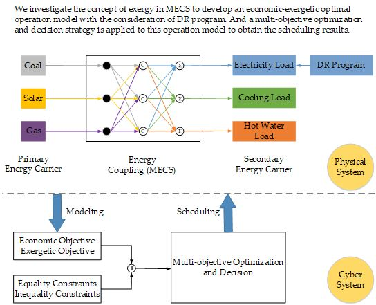
1. Introduction
- The MO optimal scheduling model of an MECS with economic and exergetic objectives are conducted and formulated into an MILP problem.
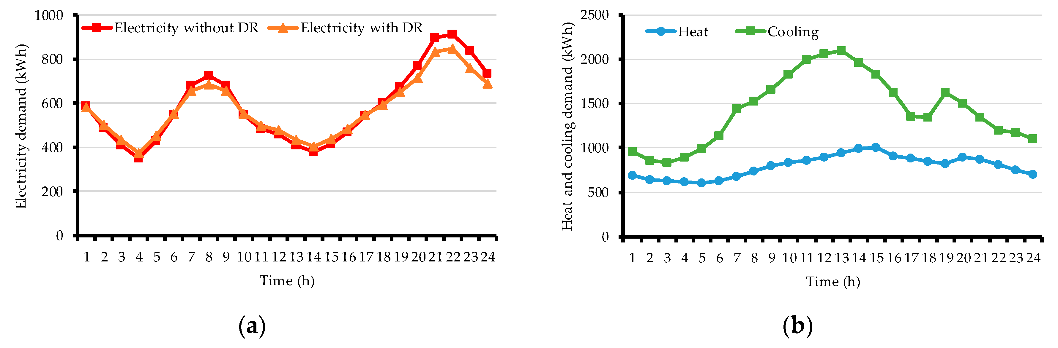
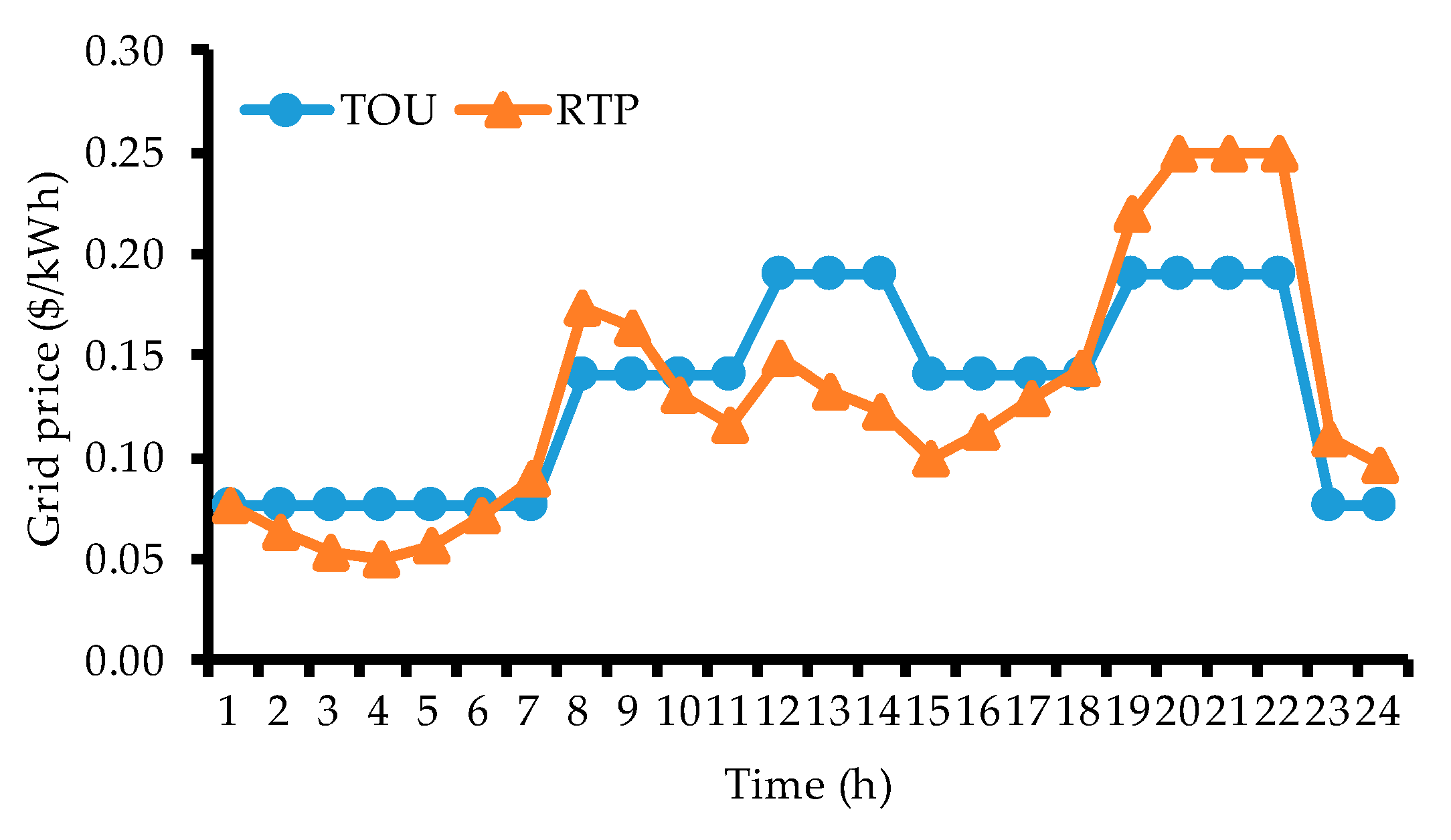
- To evaluate the performance of the DR program in an MECS, an RTP-based DR model is introduced with a dynamic pricing rate.
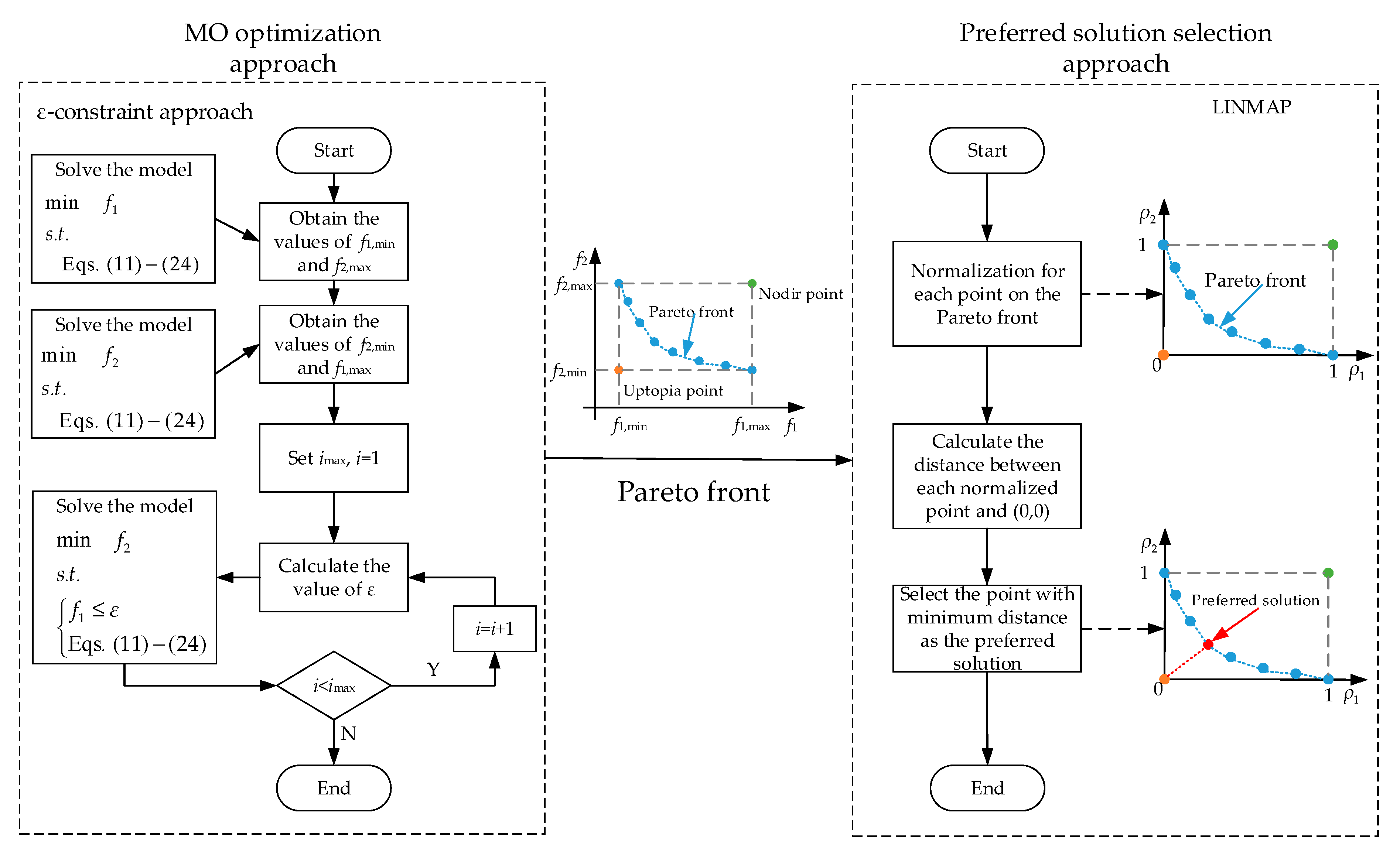
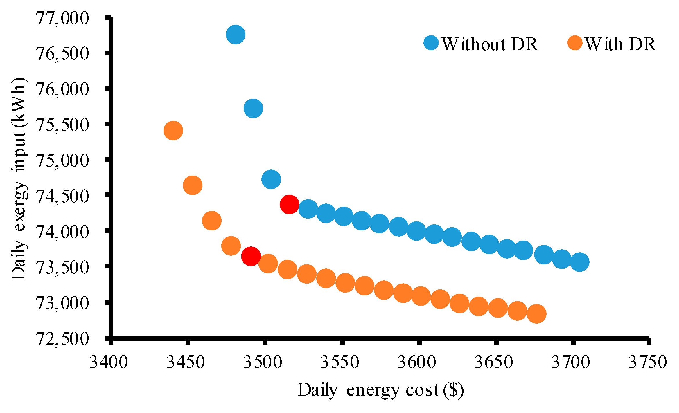
- An MO operation strategy is developed where the ε-constraint method is utilized to obtain the Pareto front, and the LINMAP approach is introduced to make a trade-off between the economic and exergetic objectives.
2. Problem Formulation
2.1. Objectives
2.1.1. Economic Objective
2.1.2. Exergetic Objective
2.2. Constraints
2.2.1. Energy Flows Constraints
2.2.2. Energy Device Constraints
2.3. RTP-Based DR Model
3. MO Operation Strategy
3.1. MO Optimization Approach
3.2. Preferred Solution Selection Approach
3.3. MO Operation Rules
4. Case Study
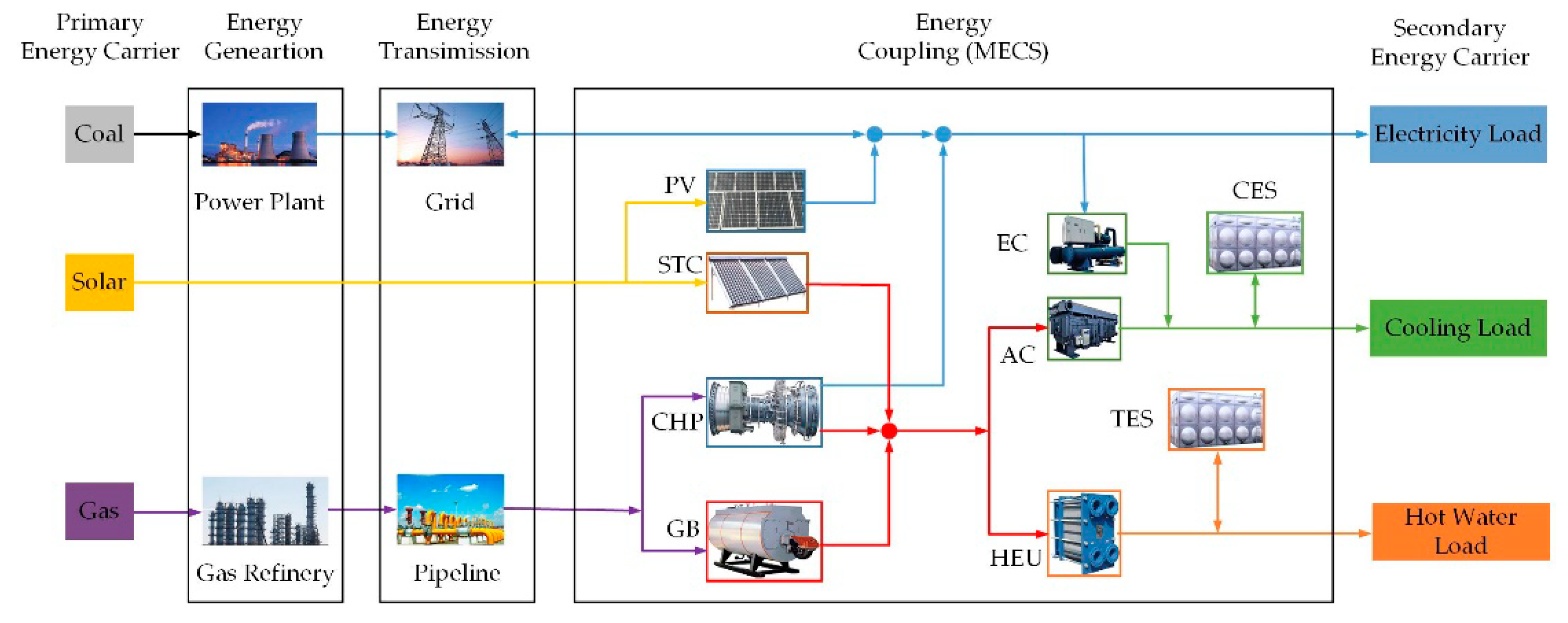
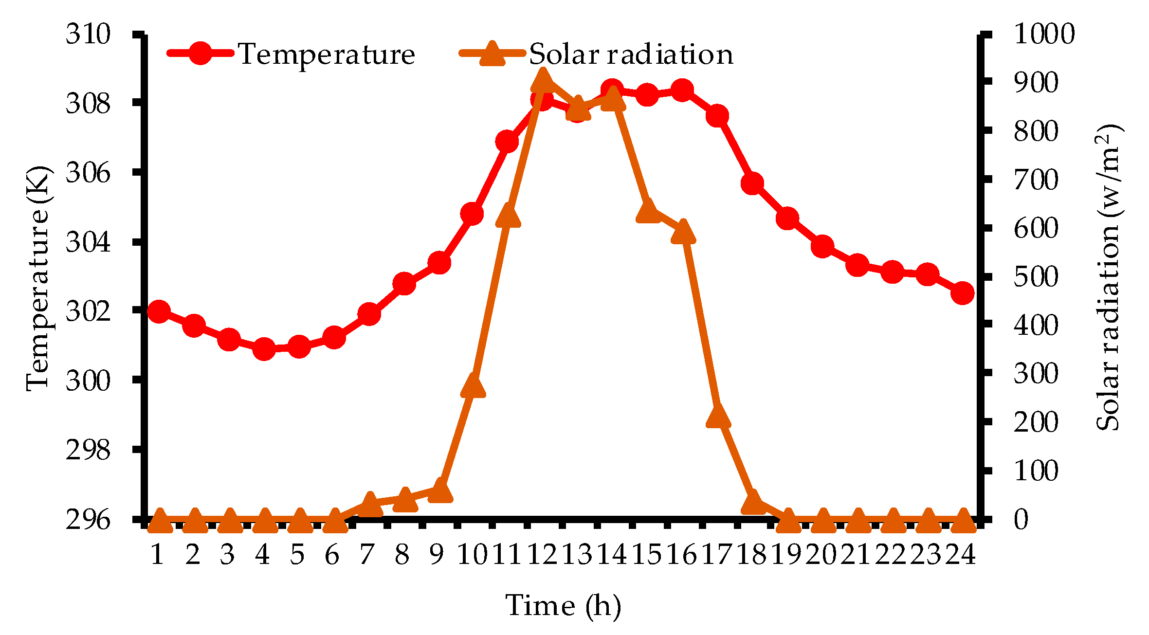
4.1. System Description
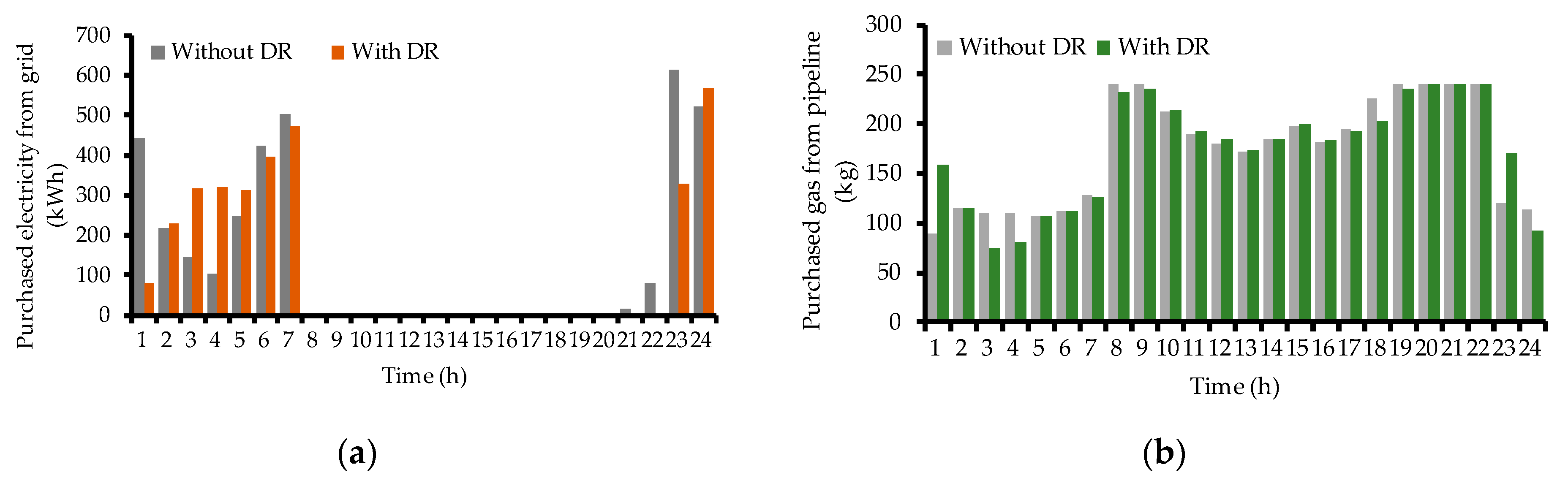
4.2. Results Analyses and Discussion
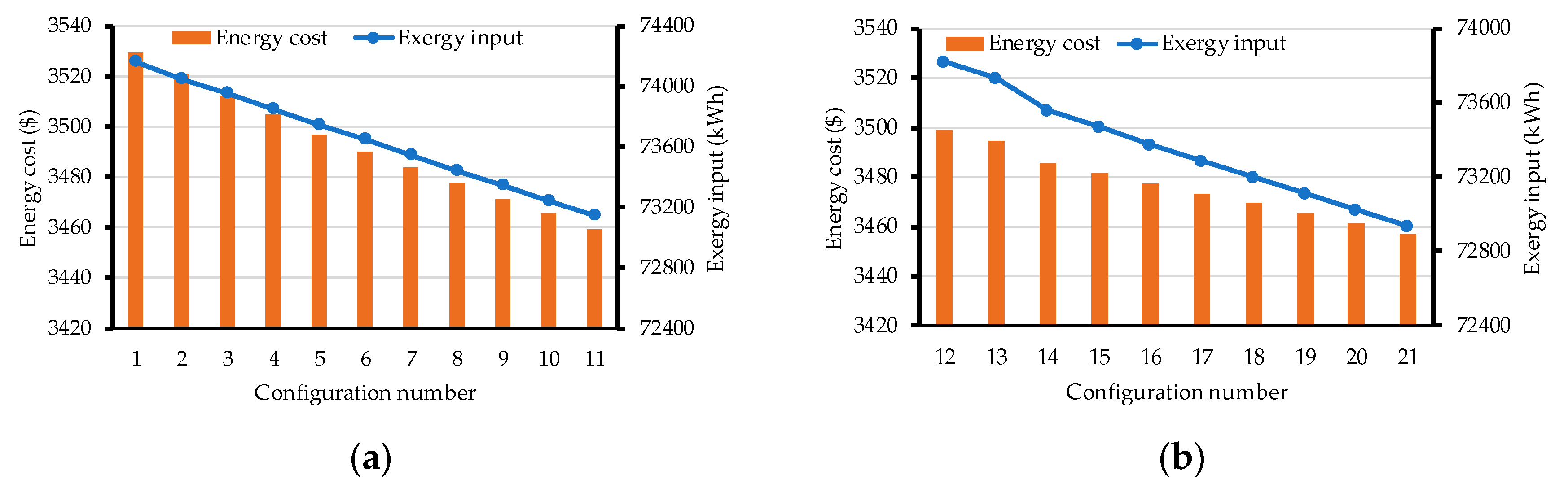
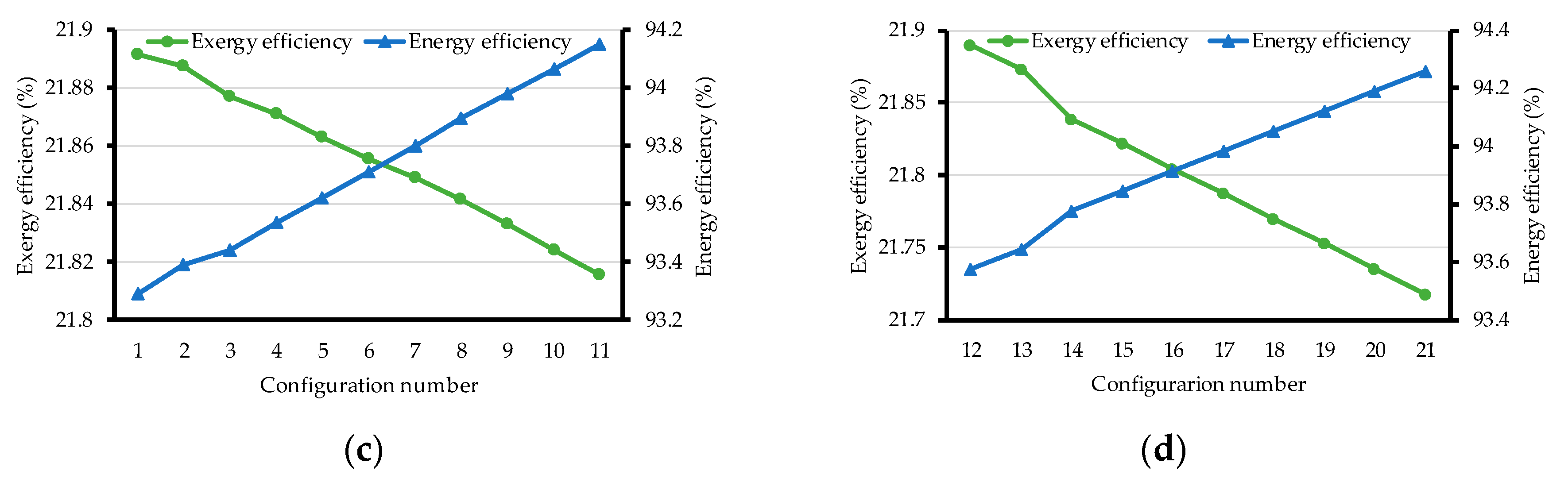
4.3. Sensitivity Experiments
5. Conclusions
Author Contributions
Funding
Conflicts of Interest
References
- Steven, C.; Arun, M. Opportunities and challenges for a sustainable energy future. Nature 2012, 488, 294–303. [Google Scholar]
- Geidl, M.; Koeppel, G.; Favre-Perrod, P.; Klöckl, B.; Andersson, G.; Fröhlich, K. Energy hubs for the future. IEEE Power Energy Mag. 2007, 5, 24–30. [Google Scholar] [CrossRef]
- Krause, T.; Andersson, G.; Fröhlich, K.; Vaccaro, A. Multiple-energy carriers: Modeling of production, delivery, and consumption. Proc. IEEE 2011, 99, 15–27. [Google Scholar] [CrossRef]
- Geidl, M.; Andersson, G. Optimal Power Flow of Multiple Energy Carriers. IEEE Trans. Power Syst. 2007, 22, 145–155. [Google Scholar] [CrossRef]
- Wang, Y.; Zhang, N.; Kang, C.; Kirschen, D.S.; Yang, J.; Xia, Q. Standardized Matrix Modeling of Multiple Energy Systems. IEEE Trans. Smart Grid 2019, 10, 257–270. [Google Scholar] [CrossRef]
- Liu, T.; Zhang, D.; Wang, S.; Wu, T. Standardized modelling and economic optimization of multi-carrier energy systems considering energy storage and demand response. Energy Convers. Manag. 2019, 182, 126–142. [Google Scholar] [CrossRef]
- Moeini-Aghtaie, M.; Abbaspour, A.; Fotuhi-Firuzabad, M.; Hajipour, E. A decomposed solution to multiple-energy carriers optimal power flow. IEEE Trans. Power Syst. 2014, 29, 707–716. [Google Scholar] [CrossRef]
- Moeini-Aghtaie, M.; Dehghanian, P.; Fotuhi-Firuzabad, M.; Abbaspour, A. Multiagent genetic algorithm: An online probabilistic view on economic dispatch of energy hubs constrained by wind availability. IEEE Trans. Sustain. Energy 2014, 5, 699–708. [Google Scholar] [CrossRef]
- Yi, J.-H.; Ko, W.; Park, J.-K.; Park, H. Impact of carbon emission constraint on design of small scale multi-energy system. Energy 2018, 161, 792–808. [Google Scholar] [CrossRef]
- Khorsand, H.; Seifi, A.R. Probabilistic energy flow for multi-carrier energy systems. Renew. Sustain. Energy Rev. 2018, 94, 989–997. [Google Scholar] [CrossRef]
- Lu, Y.; Wang, S.; Sun, Y.; Yan, C. Optimal scheduling of buildings with energy generation and thermal energy storage under dynamic electricity pricing using mixed-integer nonlinear programming. Appl. Energy 2015, 147, 49–58. [Google Scholar] [CrossRef]
- Li, Z.; Xu, Y. Optimal coordinated energy dispatch of a multi-energy microgrid in grid-connected and islanded modes. Appl. Energy 2018, 210, 974–986. [Google Scholar] [CrossRef]
- Brahman, F.; Honarmand, M.; Jadid, S. Optimal electrical and thermal energy management of a residential energy hub, integrating demand response and energy storage system. Energy Build. 2015, 90, 65–75. [Google Scholar] [CrossRef]
- Di Somma, M.; Yan, B.; Bianco, N.; Graditi, G.; Luh, P.; Mongibello, L.; Naso, V. Operation optimization of a distributed energy system considering energy costs and exergy efficiency. Energy Convers. Manag. 2015, 103, 739–751. [Google Scholar] [CrossRef]
- Torio, H.; Angelotti, A.; Schmidt, D. Exergy analysis of renewable energy-based climatisation systems for buildings: A critical view. Energy Build. 2009, 41, 248–271. [Google Scholar] [CrossRef]
- Krause, T.; Kienzle, F.; Art, S.; Andersson, G. Maximizing exergy efficiency in multi-carrier energy systems. In Proceedings of the IEEE Power and Energy Society General Meeting, Providence, RI, USA, 25–29 July 2010; pp. 1–8. [Google Scholar]
- Hepabsli, A. A Key Review on Exergetic Analysis and Assessment of Renewable Energy Resources for a Sustainable Future. Renew. Sustain. Energy Rev. 2008, 12, 593–661. [Google Scholar] [CrossRef]
- Wang, J.; Yang, Y. Energy, exergy and environmental analysis of a hybrid combined cooling heating and power system utilizing biomass and solar energy. Energy Convers. Manag. 2016, 124, 566–577. [Google Scholar] [CrossRef]
- Ahmadi, P.; Rosen, M.A.; Dincer, I. Multi-objective exergy-based optimization of a polygeneration energy system using an evolutionary algorithm. Energy 2012, 46, 21–31. [Google Scholar] [CrossRef]
- Elizondo, L.M.R.; Paap, G.; Ammerlaan, R.; Negenborn, R.R.; Toonssen, R. On the energy, exergy and cost optimisation of multi-energy-carrier power systems. Int. J. Exergy 2013, 13, 364. [Google Scholar] [CrossRef]
- Yan, B.; Di Somma, M.; Bianco, N.; Luh, P.B.; Graditi, G.; Mongibello, L.; Naso, V. Exergy-based operation optimization of a distributed energy system through the energy-supply chain. Appl. Therm. Eng. 2016, 101, 741–751. [Google Scholar] [CrossRef]
- Luis, A.A.; Edwin, R.; Francisco, S.; Victor, H. A review and analysis of trends related to demand response. Energies 2018, 11, 1617. [Google Scholar]
- Aalami, H.; Moghaddam, M.P.; Yousefi, G. Demand response modeling considering Interruptible/Curtailable loads and capacity market programs. Appl. Energy 2010, 87, 243–250. [Google Scholar] [CrossRef]
- Albadi, M.; El-Saadany, E.; Albadi, M. A summary of demand response in electricity markets. Electr. Power Syst. Res. 2008, 78, 1989–1996. [Google Scholar] [CrossRef]
- Erdinc, O.; Paterakis, N.G.; Mendes, T.D.P.; Bakirtzis, A.G.; Catalão, J.P.S. Smart Household Operation Considering Bi-Directional EV and ESS Utilization by Real-Time Pricing-Based DR. IEEE Trans. Smart Grid 2015, 6, 1281–1291. [Google Scholar] [CrossRef]
- Zhi, C.; Lei, W.; Yong, F. Real-Time Price-Based Demand Response Management for Residential Appliances via Stochastic Optimization and Robust Optimization. IEEE Trans. Smart Grid 2012, 3, 1822–1831. [Google Scholar]
- Aghamohamadi, M.; Hajiabadi, M.E.; Samadi, M. A novel approach to multi energy system operation in response to DR programs; an application to incentive-based and time-based schemes. Energy 2018, 156, 534–547. [Google Scholar] [CrossRef]
- Ma, T.; Wu, J.; Hao, L. Energy flow modeling and optimal operation analysis of the micro energy grid based on energy hub. Energy Convers. Manag. 2017, 133, 292–306. [Google Scholar] [CrossRef]
- Petela, R. Exergy of undiluted thermal radiation. Sol. Energy 2003, 74, 469–488. [Google Scholar] [CrossRef]
- Candau, Y. On the exergy of radiation. Sol. Energy 2003, 75, 241–247. [Google Scholar] [CrossRef]
- Aalami, H.; Yousefi, G.R.; Parsa Moghadam, M. A MADM-based support system for DR programs. In Proceedings of the 43rd Internatioal Universities Power Engineering Conference, Padova, Italy, 1–4 September 2008; pp. 1–7. [Google Scholar]
- Aghaei, J.; Baharvandi, A.; Rabiee, A.; Akbari, M.A. Probabilistic PMU Placement in Electric Power Networks: An MILP-Based Multi-objective Model. IEEE Trans. Ind. Inform. 2015, 11, 332–341. [Google Scholar] [CrossRef]
- Ma, T.; Wu, J.; Hao, L.; Li, D. Energy flow matrix modeling and optimal operation analysis of multi energy systems based on graph theory. Appl. Therm. Eng. 2019, 146, 648–663. [Google Scholar] [CrossRef]
- Chow, T.; Pei, G.; Fong, K.; Lin, Z.; Chan, A.; Ji, J. Energy and exergy analysis of photovoltaic–thermal collector with and without glass cover. Appl. Energy 2009, 86, 310–316. [Google Scholar] [CrossRef]
- Ahmadi, P.; Dincer, I. Exergoenvironmental analysis and optimization of a cogeneration plant system using Multimodal Genetic Algorithm (MGA). Energy 2010, 35, 5161–5172. [Google Scholar] [CrossRef]


| Parameters | Value | Parameters | Value | Parameters | Value |
|---|---|---|---|---|---|
| 0.157 | 0.9 | 0.98 | |||
| 0.8 | 4.2 | 0.02 | |||
| 0.3 | 0.8 | 0.97 | |||
| 0.45 | 0.02 | 0.95 | |||
| 0.88 | 0.98 |
| Parameters | Value/kW | Parameters | Value/kW | Parameters | Value/kW |
|---|---|---|---|---|---|
| 1000 | 100 | 0 | |||
| 200 | 1000 | 300 | |||
| 500 | 0 | 250 | |||
| −500 | 200 | 400 | |||
| 30 | 0 | 50 | |||
| 300 | 200 | 500 | |||
| 150 | 0 | 80 | |||
| 1500 | 300 | 800 |
| Case 1: Without DR | Case 2: With DR | |||||||||
|---|---|---|---|---|---|---|---|---|---|---|
| i | f1($) | f2(kWh) | d | f1($) | f2(kWh) | d | ||||
| 1 | 3704.41 | 73574.05 | 1.000 | 0.000 | 1.000 | 3676.15 | 72847.62 | 1.000 | 0.000 | 1.000 |
| 2 | 3692.63 | 73618.71 | 0.947 | 0.014 | 0.947 | 3663.75 | 72882.55 | 0.947 | 0.014 | 0.947 |
| 3 | 3680.84 | 73667.91 | 0.895 | 0.029 | 0.895 | 3651.35 | 72923.42 | 0.895 | 0.029 | 0.895 |
| 4 | 3667.59 | 73727.98 | 0.836 | 0.048 | 0.837 | 3638.95 | 72959.54 | 0.842 | 0.044 | 0.843 |
| 5 | 3657.27 | 73766.30 | 0.789 | 0.060 | 0.792 | 3626.55 | 73000.49 | 0.789 | 0.059 | 0.792 |
| 6 | 3645.49 | 73816.30 | 0.737 | 0.076 | 0.741 | 3614.15 | 73042.87 | 0.737 | 0.076 | 0.741 |
| 7 | 3633.70 | 73864.69 | 0.684 | 0.091 | 0.690 | 3601.75 | 73086.82 | 0.684 | 0.093 | 0.690 |
| 8 | 3621.91 | 73913.88 | 0.632 | 0.107 | 0.641 | 3589.35 | 73132.19 | 0.632 | 0.111 | 0.641 |
| 9 | 3610.13 | 73963.08 | 0.579 | 0.122 | 0.592 | 3576.95 | 73180.72 | 0.579 | 0.129 | 0.593 |
| 10 | 3598.34 | 74012.27 | 0.526 | 0.137 | 0.544 | 3564.55 | 73229.62 | 0.526 | 0.148 | 0.547 |
| 11 | 3586.56 | 74061.46 | 0.474 | 0.153 | 0.498 | 3552.15 | 73281.93 | 0.474 | 0.169 | 0.503 |
| 12 | 3574.77 | 74110.66 | 0.421 | 0.168 | 0.453 | 3539.75 | 73337.80 | 0.421 | 0.191 | 0.462 |
| 13 | 3562.98 | 74159.85 | 0.368 | 0.184 | 0.412 | 3527.35 | 73401.26 | 0.368 | 0.215 | 0.427 |
| 14 | 3551.20 | 74209.47 | 0.316 | 0.199 | 0.373 | 3514.95 | 73464.81 | 0.316 | 0.240 | 0.397 |
| 15 | 3539.41 | 74263.74 | 0.263 | 0.216 | 0.341 | 3502.55 | 73546.73 | 0.263 | 0.272 | 0.378 |
| 16 | 3527.63 | 74318.07 | 0.211 | 0.233 | 0.314 | 3490.15 | 73644.09 | 0.211 | 0.310 | 0.374 |
| 17 | 3515.84 | 74389.45 | 0.158 | 0.256 | 0.301 | 3477.74 | 73793.13 | 0.158 | 0.367 | 0.400 |
| 18 | 3504.05 | 74731.77 | 0.105 | 0.363 | 0.378 | 3465.34 | 74162.12 | 0.105 | 0.511 | 0.522 |
| 19 | 3492.27 | 75732.11 | 0.053 | 0.677 | 0.679 | 3452.94 | 74642.98 | 0.053 | 0.698 | 0.700 |
| 20 | 3480.48 | 76761.51 | 0.000 | 1.000 | 1.000 | 3440.54 | 75420.63 | 0.000 | 1.000 | 1.000 |
| # | e(t,t) | e(t,k) | # | e(t,t) | e(t,k) |
|---|---|---|---|---|---|
| 1 | 0 | 0.01 | 12 | −0.20 | 0 |
| 2 | −0.04 | 0.01 | 13 | −0.20 | 0.005 |
| 3 | −0.08 | 0.01 | 14 | −0.20 | 0.015 |
| 4 | −0.12 | 0.01 | 15 | −0.20 | 0.020 |
| 5 | −0.16 | 0.01 | 16 | −0.20 | 0.025 |
| 6 | −0.20 | 0.01 | 17 | −0.20 | 0.030 |
| 7 | −0.24 | 0.01 | 18 | −0.20 | 0.035 |
| 8 | −0.28 | 0.01 | 19 | −0.20 | 0.040 |
| 9 | −0.32 | 0.01 | 20 | −0.20 | 0.045 |
| 10 | −0.36 | 0.01 | 21 | −0.20 | 0.050 |
| 11 | −0.40 | 0.01 |
© 2019 by the authors. Licensee MDPI, Basel, Switzerland. This article is an open access article distributed under the terms and conditions of the Creative Commons Attribution (CC BY) license (http://creativecommons.org/licenses/by/4.0/).
Share and Cite
Huang, Y.; Li, S.; Ding, P.; Zhang, Y.; Yang, K.; Zhang, W. Optimal Operation for Economic and Exergetic Objectives of a Multiple Energy Carrier System Considering Demand Response Program. Energies 2019, 12, 3995. https://doi.org/10.3390/en12203995
Huang Y, Li S, Ding P, Zhang Y, Yang K, Zhang W. Optimal Operation for Economic and Exergetic Objectives of a Multiple Energy Carrier System Considering Demand Response Program. Energies. 2019; 12(20):3995. https://doi.org/10.3390/en12203995
Chicago/Turabian StyleHuang, Yu, Shuqin Li, Peng Ding, Yan Zhang, Kai Yang, and Weiting Zhang. 2019. "Optimal Operation for Economic and Exergetic Objectives of a Multiple Energy Carrier System Considering Demand Response Program" Energies 12, no. 20: 3995. https://doi.org/10.3390/en12203995