Improving the Performance of a Dual Kalman Filter for the Identification of PEM Fuel Cells in Impedance Spectroscopy Experiments

Abstract

In this paper, the Dual Kalman Filter (DKF) is used for the parametric identification of an RC model of a Polymer Electrolyte Membrane Fuel Cell (FC) stack. The identification is performed for diagnostic purposes, starting from time-domain voltage and current signals in the framework of Electrochemical Impedance Spectroscopy (EIS) tests. Here, the sinusoidal input of the tests makes the identification of DKF parameters challenging. The paper analyzes the filter performance and proposes a possible approach to address the filter tuning to let it work with FC operating either in normal conditions or in the presence of drying and flooding fault conditions, or in fuel starvation mode. The analysis is mainly performed in a simulated environment, where the Fouquet model is used to simulate the FC. Some criteria to tune the filter are derived from the analysis and used also with experimental data produced by some EIS tests, to achieve the best estimate in constrained conditions. The results show that the DKF can be turned into a valuable tool to identify the model parameters even with signals developed for other scopes. The identification results envisage the possibility of assisting the model-based FC diagnosis by means of a very simple tool that can run on a low-cost embedded device. Indeed, the simplicity of the filter approach and a lightweight implementation allow the deployment of the algorithm in embedded solutions.

1. Introduction

Fuel cells (FCs) are effective energy conversion devices, used in various application branches—for instance, systems power auxiliaries, smart grids [1], automotive applications and transportation systems [2], and portable devices. Many FC technologies are available. Solid Oxide Fuel Cell [3] and Polymer Electrolyte Membrane FC (PEMFC) [4] are examples of hydrogen-based FC technologies. Recently, some alternative liquid-based FCs are being considered for perspective applications, such as direct ammonia FC [5] and acid–base FC [6]. Among these, PEMFCs, compared to other types of FC, show various advantages. For instance, the high stack power density (greater than 1.3 kW kg${}^{-1}$), the absence of corrosion problems typical of other cells with liquid electrolyte, the relative simplicity of construction and, finally, the fast cold start (within a minute). These characteristics allowed the development of PEMFCs for space applications and automotive applications [4], as well as for stationary generation/cogeneration [7] and for portable generation [8].

Unfortunately, one of the main obstacles to the widespread diffusion of this technology is the reliability of the stack, whose performance and life span depend strongly on a series of phenomena regarding both the membrane and the reactants [9,10]. For instance, the membrane could be subject to drying and flooding faulty conditions (i.e., lack or excess of water) when the water removal from the FC is not properly managed [11]. Another typical fault condition is the fuel starvation, causing an irreversible reaction in the cell [12]. All these faults lead to a premature degradation of the FC. For this reason, diagnosis has a crucial role in order to extend the overall lifetime of a cell and improve its reliability. Many attempts have been made in literature to characterize faults [13], especially in the framework of water management [14], aimed at developing monitoring and prognostic methods [15,16].

In recent years, the fault detection calls for the online operability of this analysis, which can be performed through a parametric identification of a PEMFC circuit model. The most popular approaches for online monitoring and diagnostics are based on the FC polarization characteristics, i.e., the voltage-to-current curve [17]. Despite this, some European projects have shown the online applicability of diagnostic techniques based on the classical laboratory analysis called Electrochemical Impedance Spectroscopy (EIS). The EIS is suitable for any electrochemical device, including batteries [18], and it is usually performed with expensive laboratory equipment. Stimulating the device with an appropriate input current signal, the EIS allows to analyze any electrochemical device through the values of the impedance, which is computed on the basis of the measured output voltage. Once the impedance plot is obtained, a parametric identification of the FC system, based on the overall impedance plot, allows to make diagnosis [19]. The EIS is often performed with sinusoidal input signals offline, i.e., by disconnecting the FC from the load. In the aforementioned projects, the powerful capabilities of the FC interface DC-DC converter are exploited to inject sinusoidal current perturbation when the fuel cell is operating online [20].

In this paper, a time-domain identification method of a PEMFC system, based on the use of the time-domain sinusoidal input signals in an online EIS experiment [21], is proposed and optimized in terms of convergence performance. The method, suitable for implementation on small-cost embedded devices, is based on the Dual Kalman Filter (DKF) [22,23]. This filter is well-known and widely used in literature for various applications, including electrochemical ones. For instance, it is often used in battery management systems for the online estimation of the battery’s state of charge [24]. The literature highlights that the best performance in term of estimation is achieved for strong time-varying input signals, e.g., a typical automotive driving schedule. In this paper, the framework proposed deeply differs from the typical DKF application, because the input signals are not designed to work with the DKF, and it is aimed at “scavenging” the information contained in the large amount of time-domain data available from online acquisition of EIS for PEMFC system. These data are typically postprocessed to achieve frequency-domain information. Critical convergence issues are documented in FC subject to a sinusoidal input with a test case, where if the FC is simulated by a rough model consisting of linear first-order dynamic circuits with constant parameters [25].

The method and the study carried out in this work are aimed at overcoming these problems in a more realistic framework. The PEMFC is represented by an enhanced first-order circuit model, characterized by frequency-varying parameters. A suitable choice of aggregate parameters is adopted to improve the identification capabilities of the filter, as suggested in [26]. Frequency-dependent parameters are identified, frequency by frequency. The peculiar shape of input signals requires a suitable setting of the filter parameters, such as the initial covariance matrix and the sampling frequency, to let the DKF work effectively with these signals. A novel approach for the determination of an optimal initial covariance matrix and sampling frequency is proposed, allowing to get accurate identification results over a wide frequency range. Three realistic FC operating cases are considered: Normal FC operation; membrane drying; and flooding. The FC response is simulated using literature data and a complex PEMFC model, called Fouquet model [27]. The frequency-dependent identification results reflect the operating condition, allowing, in perspective, a preliminary FC diagnosis. An example of application of the proposed method on experimental data is also provided. Here, the FC normal and fuel starvation operating conditions are considered. The example confirms the validity of the identification approach.

The paper is organized as follows. Section 2 introduces equivalent circuit models of an FC used for simulation and identification scopes, Section 3 outlines the identification approach and discusses the main identification variables involved, Section 4 deals with the optimal choice of initial covariance and sampling frequency of the DKF obtained on the basis of the identification results in a realistic simulated environment, and Section 5 presents the identification results in an experimental case, showing the effectiveness of the approach. Finally, Section 6 concludes the papers and outlines possible future perspectives.

2. Fuel Cell Models

2.1. Fouquet Model

An accurate PEMFC model, often used in EIS analysis, is represented by the Fouquet impedance (see Figure 1) This impedance includes the complex-valued Warburg element and a Constant Phase Element (CPE), defined as follows:

$$\begin{array}{cc}\hfill {\dot{Z}}_{\mathrm{CPE}}& =\frac{1}{Q{\left(j\omega \right)}^{\varphi }},\hfill \end{array}$$

(1)

$$\begin{array}{cc}\hfill {\dot{Z}}_{\mathrm{W}}& =R_{\mathrm{d}}\frac{tanh\sqrt{j\omega {\tau }_{\mathrm{d}}}}{\sqrt{j\omega {\tau }_{\mathrm{d}}}},\hfill \end{array}$$

(2)

where $\omega =2\pi f$ is the angular frequency; Q and $\varphi$ define the CPE, which models the behavior of electrodes in the case of rough and porous surfaces (with $\varphi \in [-1;1]$); and $R_{\mathrm{d}}$ represents the losses due to the diffusion of reactants, characterized by the time constant ${\tau }_{\mathrm{d}}$. The Fouquet impedance is then defined by

$$\dot{Z}=R_{\mathsf{\Omega }}+\frac{{\dot{Z}}_{\mathrm{CPE}}(R_{\mathrm{ct}}+{\dot{Z}}_{\mathrm{W}})}{{\dot{Z}}_{\mathrm{CPE}}+R_{\mathrm{ct}}+{\dot{Z}}_{\mathrm{W}}}.$$

(3)

Here, $R_{\mathsf{\Omega }}$ represents the losses due to the resistance of the electrolyte to the flow of protons, and $R_{\mathrm{ct}}$, named the charge transfer resistance, is the resistance at the interface electrode/electrolyte to the flow of charges. The impedances ${\dot{Z}}_{\mathrm{CPE}}$, ${\dot{Z}}_{\mathrm{W}}$ and the resistances $R_{\mathrm{d}}$, $R_{\mathsf{\Omega }}$, and $R_{\mathrm{ct}}$ are measured in ohms ($\mathsf{\Omega }$),${\tau }_{\mathrm{d}}$ is measured in seconds ($\mathrm{s}$) and Q in Siemens ($\mathrm{S}$). This assumption requires that ${\left(j\omega \right)}^{\varphi }$ be adimensional.

The Fouquet model will be used in the following to simulate the behavior of a PEMFC, by using the set of data identified in [28] from various experiment performed in [27], where an FC stack, made of 6 cells, was operated in normal conditions as well as in membrane drying or flooding conditions. The cell active area is 150 $\mathrm{c}$$\mathrm{m}$${}^2$, with an operating current of 70 $\mathrm{A}$, at a constant temperature of 60 ${}^{\circ }\mathrm{C}$, at atmospheric pressure on both sides, with stoichiometries at 1.2 on anode side and 4.0 on cathode side. The faults were induced by modifying the relative humidity of the gas. In particular, to trigger the flooding, the relative humidity was kept constant at 50% on cathode and 70% on anode. For the drying condition, the inlet gas was kept at 10% on anode and 15% on cathode. The data used to simulate the FC time-domain response are reported in

Table 1. Fouquet model parameters in various fuel cell (FC) stack conditions, as reported in [28].

	${\mathit{R}}_{\mathbf{\Omega }}$ ($\mathbf{m}\mathbf{\Omega }$)	${\mathit{R}}_{\mathbf{ct}}$ ($\mathbf{m}\mathbf{\Omega }$)	Q ($\mathbf{S}$)	$\mathit{\varphi }$	${\mathit{R}}_{\mathbf{d}}$ ($\mathbf{m}\mathbf{\Omega }$)	${\mathit{\tau }}_{\mathbf{d}}$ ($\mathbf{s}$)
Normal	4.5	8.1	1.8056	0.8419	3.6	0.1919
Drying	9.3	12.1	0.8741	0.8389	10.5	0.3638
Flooding	4.1	16.7	0.9712	0.8155	30.9	0.1007

. The response of the model is represented in Figure 2.

2.2. First-Order Linear Fuel Cell Model

Despite its accuracy and widespread application, the Fouquet model is defined in frequency domain and is not characterized by time-domain equations in closed form. The presence of the CPE and of the Warburg impedance leads to a complicated and computationally ineffective use of the model in the time domain, requiring approaches such as fractional order model [29]. Conversely, linear lumped circuits, made of linear resistors and capacitors, are an effective model for electrochemical devices for online control scopes. They can be easily and effectively used both in frequency and in time domain. Due to their simplicity, they could be less accurate with respect to Fouquet model, unless a large number of lumped elements are used.

Figure 3 shows the simplest version of the Randles cell, hereafter called RRC impedance (or RRC model). In this circuit, the resistance $R_0$, measured in $\mathsf{\Omega }$, models the ohmic losses caused by the overlap of the ionic resistance of the electrolyte and of the electric resistances caused by electrodes and connections. Among these, the dominant losses are those related to transport of protons in the electrolyte resistance. On the other hand, the resistance $R_1$, measured in $\mathsf{\Omega }$, models the charges’ flow through the electrode/electrolyte interface and it is closely linked to kinetics of reactions. It is also necessary to consider that, when different materials are in contact, a concentration of charges is stored on their surfaces, adjusting the transfer of charges from one side to the other. Diffusive effects, reactions between electrons and charges, or changes in the applied voltage can influence the dynamics of a PEMFC generating a capacitive behavior. For this reason, the capacitance $C_1$, measured in Farad ($\mathrm{F}$), is introduced [18].

The model is described by the following state-space and output equations:

$$\begin{array}{cc}\hfill \frac{d{v}_c}{dt}\left(t\right)& =-\frac{1}{R_1{C}_1}{v}_c\left(t\right)-\frac{1}{C_1}i\left(t\right),\hfill \end{array}$$

(4)

$$\begin{array}{cc}\hfill v_t\left(t\right)& =v_c\left(t\right)-R_{0}i\left(t\right),\hfill \end{array}$$

(5)

where t is the time, $v_c$ is the voltage across the capacitor, $v_t$ is the voltage across the FC terminals (oriented according to $v_c$), and i is the current (active sign convention is used). In the equations above, a process noise and a measurement noise can be added to represent the uncertainty on input signal and measurements.

Converting the model (4) and (5) into the discrete-time model for the implementation on a computer, we get

$$\begin{array}{cc}\hfill v_{c,k+1}& =e^{-\frac{\Delta t}{R_1{C}_1}}{v}_{c,k}-R_1\left(1-e^{-\frac{\Delta t}{R_1{C}_1}}\right)i_k,\hfill \end{array}$$

(6)

$$\begin{array}{cc}\hfill v_{t,k}& =v_{c,k}-R_0{i}_k,\hfill \end{array}$$

(7)

where the subscript k indicates the variable sampled at the discrete time instant $t_k$.

It is useful to introduce the following quantities:

$$\begin{array}{cc}\hfill f_c& =\frac{1}{\tau }=\frac{1}{R_1{C}_1},\hfill \end{array}$$

(8)

$$\begin{array}{cc}\hfill \alpha & =e^{-\frac{\Delta t}{R_1{C}_1}},\hfill \end{array}$$

(9)

$$\begin{array}{cc}\hfill \beta & =R_1(1-\alpha ),\hfill \end{array}$$

(10)

that allow to rewrite Equations (6) and (7) as follows:

$$\begin{array}{cc}\hfill v_{c,k+1}& =\alpha v_{c,k}-\beta i_k,\hfill \end{array}$$

(11)

$$\begin{array}{cc}\hfill v_{t,k}& =v_{c,k}-R_0{i}_k.\hfill \end{array}$$

(12)

Considering $R_0$, $\alpha$, and $\beta$ as primal parameters of the model, it is easy to map them into the original parameters $R_1$ and $C_1$, using the following formulas:

$$\begin{array}{cc}\hfill R_1& =\frac{\beta }{1-\alpha },\hfill \end{array}$$

(13)

$$\begin{array}{cc}\hfill C_1& =-\frac{\Delta t}{R_{1}log\alpha }.\hfill \end{array}$$

(14)

The linearity of the model allows it to be used in a very simple way in time-domain numerical schemes, useful for a time-domain identification approach. Obviously, in the presence of a small number of circuit elements having constant value, a considerable deviation between the semicircular Nyquist plot of the RRC circuit and the one typical of an FC is observed. In the following, $R_1$ and $C_1$ are assumed as frequency-varying, to improve the RRC model accuracy. $R_0$ is constant, and its value can be retrieved by inspecting the intersection of the impedance spectrum with the real axis (

Table 2. $R_0$ value in different operating conditions.

Operating Condition	${\mathit{R}}_0$ ($\mathbf{m}$$\mathbf{\Omega }$)
Normal	4.5
Drying	9.3
Flooding	4.1

).

3. Time-Domain Identification in the EIS Framework

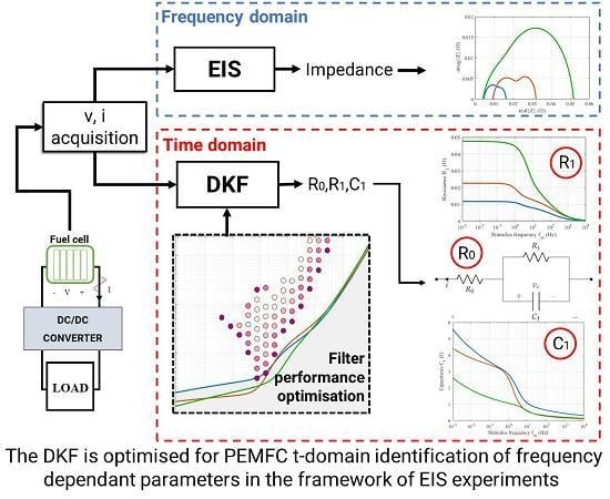
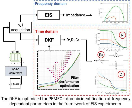
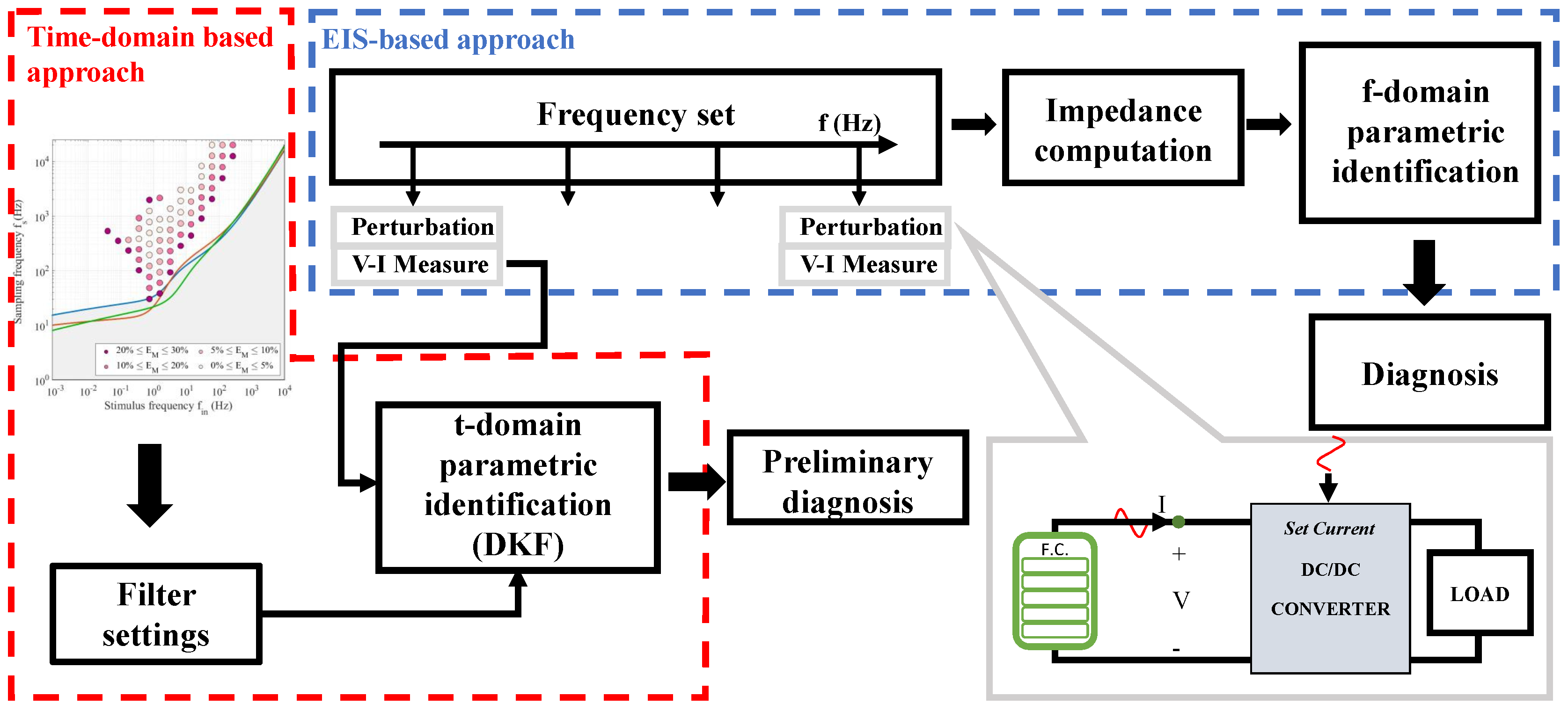
The flow-chart in Figure 4 depicts how to integrate the parametric identification technique optimized in this work (red zone) into the EIS-based diagnostic framework, in which a frequency-domain parametric identification (blue zone) is associated to a diagnostic tool. The EIS-based fault detection is performed by executing multiple steps. First, the duty cycle of the DC-DC converter is perturbed with the goal of generating a small-amplitude sinusoid superimposed to the actual DC output current of the FC. The FC voltage (V) and current (I) are sampled and suitably processed with a Fast Fourier Transform (FFT), allowing the computation of the FC impedance [21]. This procedure is repeated at various input frequencies. The whole impedance spectrum allows one to perform an equivalent circuit model identification, and, consequently, a fault detection. The fault detection stage begins after the whole impedance spectrum is acquired and the equivalent circuit model are extracted.

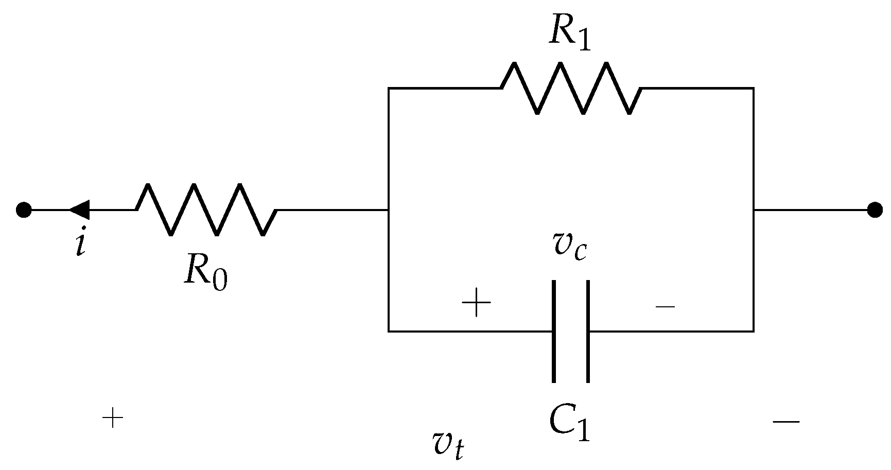
A complementary approach supporting the EIS-based one can be established by exploiting time-domain data from the I-V measurement step (red dashed box). In particular, time-domain I and V signals can be used by a DKF to perform a time-domain-based parametric identification of a very simple circuit model, such as the RRC model, where the parameters are functions of the input frequency. The identification is performed, frequency by frequency, in a sequential way, allowing a preliminary diagnosis based on the RRC parameters. The information on the parameter variation with respect to nominal condition is available at a very early stage, even after one or few I-V signals are acquired. This information is harvested from the time-domain signals before the whole data acquisition is performed. For this reason, this strategy appears suitable for increasing the diagnostic capabilities of the overall system, based on parametric identification.

The use of a low-order model within the DKF algorithm has a direct impact on the dimension of the matrices involved in the identification process. It follows that the number of floating point operations required by the identification is limited, reducing the overall computational burden. Despite the effective computational performance, the setting of the DKF to achieve satisfactory identification results in this peculiar context is a challenging task because of the input signals characteristics required by the EIS. This is worth investigating in detail.

3.1. Dual Kalman Filter

The DKF is a time-domain approach to perform the estimate of state and parameters of a dynamic system. The mathematical formulation of the DKF is based on the discrete state-space model of the system, allowing to update the state and parameter estimate by using their previous values and suitable correction terms. Indeed, for the estimate of the state, the discretized equations are used for the FC state output and the goal of the filter is to overlap the output of the model with the measured output of the FC. This is achieved by stimulating both the system and the model with the same input, and by measuring the output and comparing them. The estimate output is given in terms of state and output variable values and covariance of these two. These values, together with the system input and output measurements, are used recursively to produce an updated estimate. In particular, the covariance of measurements and state are used to calculate the Kalman gain, which is used to give more weight to the state estimate or to the system measurements. The same concept can be applied to the parameters estimate. In this case, it is necessary to provide a space-state representation of the parameters evolution. This is modeled as a random walk, where the updated parameters vector is obtained by adding a Gaussian noise to the previous values. In this way, the parameters are assumed to vary slowly and the added noise is used to account for uncertainty of the values.

The DKF used for the identification of the linear RRC impedance under stimuli typical of an EIS experiment was implemented as described in [24]. The voltage across the capacitor $C_1$ is the state variable and the parameter vector to be identified is $\theta ={[R_0,\alpha ,\beta ]}^T$, from which $R_1$ and $C_1$ can be found using Equations (13) and (14).

3.2. Sequential Identification with DKF

The input signal of the EIS experiment is a sequence of N sinusoidal stimuli. Each sinusoid is characterized by the value of its frequency $f_{in,i}$, with $i=1\dots N$. Here, the sequence of sinusoids goes from the highest frequency, $f_{in,N}$, to the lowest, $f_{in,1}$. The reversed sequence of stimuli allows to perform the identification process in a sequential way, using the principle adopted in [25] for a set of constant parameters. Indeed, first $R_0$ is identified at high frequency and kept constant in the successive identifications of $\alpha$ and $\beta$, which are the frequency-dependent parameters. In other words, for each frequency stimulus $f_{in,i}$, the values ${\alpha }_i=\alpha \left(f_{in,i}\right)$ and ${\beta }_i=\beta \left(f_{in,i}\right)$ have to be found. To do this, the filter parameters need to be rearranged frequency by frequency because the same filter initialization at each frequency does not allow convergence and a good parameter estimation for all frequencies.For these reasons, a tuning of the filter, frequency-by-frequency, is required to achieve a good identification result.

3.3. Filter Parameters and Response to Sinusoidal Input

The DKF performance is characterized by many parameters. For instance, the initial covariance vector, namely, ${\sigma }^2$, whose components ${\sigma }_{R_0}^2$, ${\sigma }_{\alpha }^2$, ${\sigma }_{\beta }^2$ are associated to parameters to be identified. The covariance matrix ${\sigma }^2$ impacts in a significant way on the response of the algorithm. In general, the higher the covariance associated to the j-th parameter, the faster, and more unstable, the response on the j-th parameter. For the sake of simplicity, hereafter, instead of referring to the covariance values ${\sigma }^2$, their logarithm $\gamma$ is given: $\gamma ={log}_{10}\left({\sigma }^2\right)$. Two more parameters have to be chosen carefully. First, the sampling frequency $f_s$, then, the acquisition buffer size $N_{smp}$. The first one deeply affects the identifiability of the parameters. 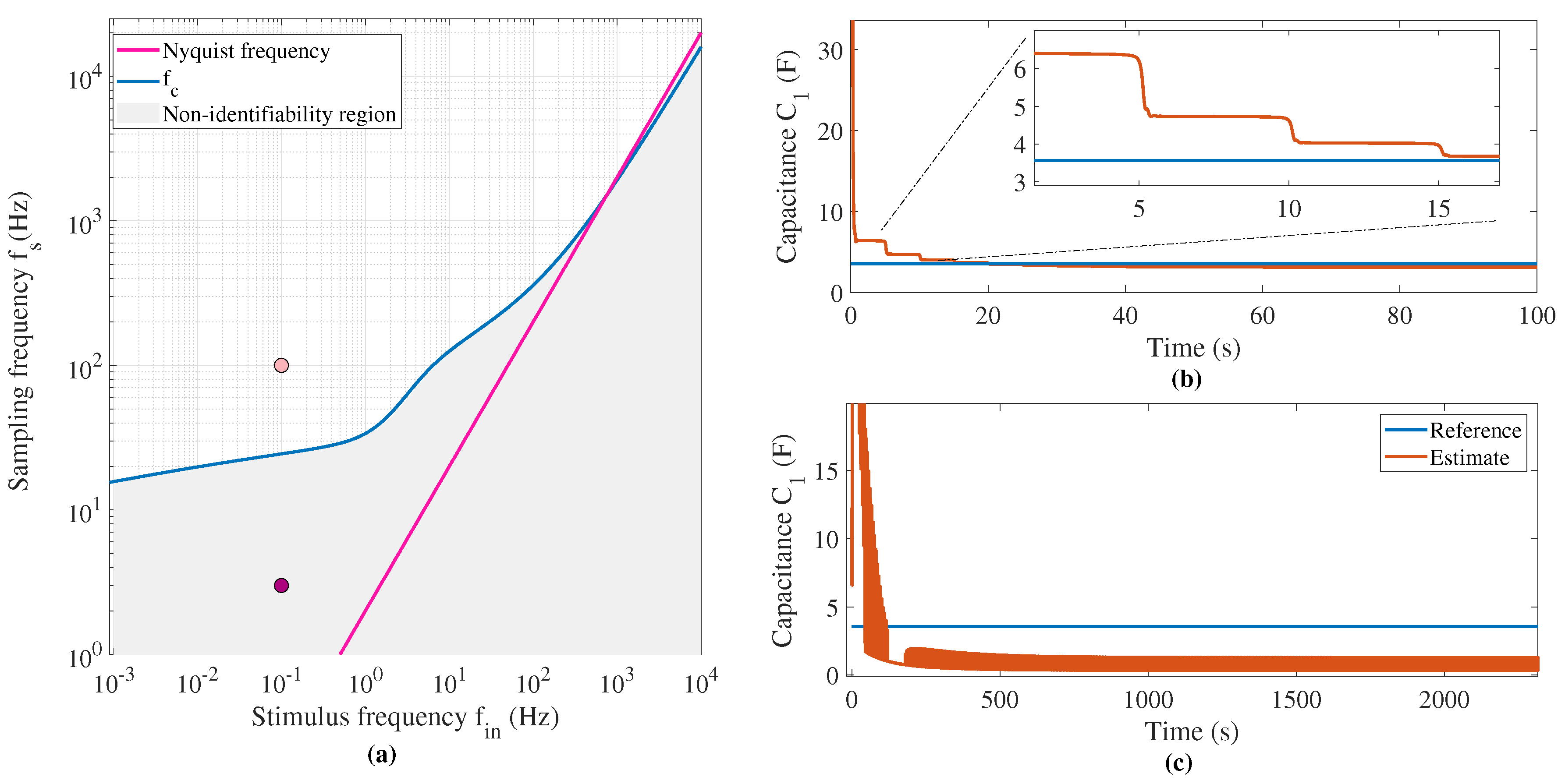Figure 5 shows the identification of the parameter $C_1$ for a zero-mean input sinusoid at frequency $f_{in}=0.1\mathrm{Hz}$ and for various sampling frequencies in normal conditions where $f_c=25\mathrm{Hz}$. In these tests, the covariance values are kept constant. Figure 5c shows the estimation obtained for sampling below the characteristic frequency. The filter cannot identify the correct parameter as it is not able to describe the system transient being $f_c\gg f_s$.

Raising the sampling frequency to 100 $\mathrm{Hz}$ allows to correctly estimate the parameter (Figure 5b). Here, $f_c\ll f_s$, and the system dynamics can be described by the inner model of the filter in an appropriate way. The inset in the figure also shows that the stepwise evolution of the estimation is led on by the number of observed semiperiods of the input signal, namely, the number of zero-crossing points of the sampled sinusoid. In other words, when a change in the sign of the current is detected, an evolution of the estimate is observed.

This behavior of the filter leads to two practical considerations. First, the mean value of the DC operating point of the current has to be subtracted from the measured value. This is not considered to be a problem, since the operating point of the fuel cell is known, provided that the FC is in stationary conditions. Second, the acquisition buffer size $N_{smp}$ could indirectly affect the result of the identification, as it modulates the number of zero-crossing points that would produce an evolution in the estimation.

Here, the considered maximum sampling frequency was fixed to $f_{s,M}=20\mathrm{k}\mathrm{Hz}$, and the number of samples was set to $N_{smp}=10$ kSample, so that the time window to perform the estimate is determined as $N_{smp}/f_s$. These values are compatible with the specification of low-cost embedded systems performing the voltage and current measurements. The discussed behavior of the filter leads to the definition of an identifiability domain area, represented in Figure 5a, and described by the following conditions linking the sampling frequency, the characteristic frequency, and the input stimulus frequency:

$$\left\{\begin{array}{c}{f}_s>2f_{in}\hfill \\ f_c<f_s<f_{s,M}\hfill \\ 1\mathrm{m}\mathrm{Hz}<f_{in}<10\mathrm{k}\mathrm{Hz}.\hfill \end{array}\right.$$

(15)

The first equation in (15) is the Nyquist rate condition, allowing to correctly sample the input sinusoid. The second identifies the area where the estimation is feasible, and it is based on the previously discussed filter behavior. The last equation in (15) identifies the frequency range where the EIS experiments are taken. This set of conditions allows us to bound in a narrower area the analysis of the filter response. The part of the plane where the identification is unfeasible is highlighted in gray color in Figure 5a.

4. Identification Performance Analysis in Simulated Environment

The response of the filter was analyzed on the $f_{in}-f_s$ plane, in a simulated environment, where the behavior of the FC is simulated by running the Fouquet model.

Here, the Fouquet model is stimulated with a single tone, and its output is brought back into the time-domain through an Inverse Fast Fourier Transform (IFFT) to obtain the waveform of the voltage response. The impact of the covariance on the identification performance is evaluated by sampling the $f_s-f_{in}$ domain in a suitable way. For each input frequency $f_{in}$, the characteristic frequency $f_c$ has to be evaluated. Then, the sampling frequency axis $f_s$ is sampled, starting from $f_c$ up to the maximum sampling frequency $f_{s,M}$.

The identification performance on the parameter p in the operating condition x, namely $p_x$, is evaluated by means of the error $E_{p,x}$ of p with respect to its theoretical value $p_x^{\left(th\right)}$—being $p\in \{R_0,R_1,C_1\}$ and $x=\{N,D,F\}$ for normal, drying, or flooding operating conditions. The theoretical value $p_x^{\left(th\right)}$ is extracted on the basis of frequency-domain impedance data after an assessed identification procedure based on the known Fouquet model. All errors, either in normal or in faulty operating conditions, are normalized with respect to the theoretical value in normal conditions, $p_N^{\left(th\right)}$, to get a percentage error. In formulas:

$$\begin{array}{cc}\hfill E_{R_0,x}& =\frac{|R_{0,x}^{\left(th\right)}-{\widehat{R}}_{0x}|}{R_{0,N}^{\left(th\right)}},\hfill \end{array}$$

(16)

$$\begin{array}{cc}\hfill E_{R_1,x}& =\frac{|R_{1,x}^{\left(th\right)}-{\widehat{R}}_{1x}|}{R_{1,N}^{\left(th\right)}},\hfill \end{array}$$

(17)

$$\begin{array}{cc}\hfill E_{C_1,x}& =\frac{|C_{1,x}^{\left(th\right)}-{\widehat{C}}_{1x}|}{C_{1,N}^{\left(th\right)}},\hfill \end{array}$$

(18)

where $\widehat{p}$ stands for the identification result.

The maximum relative error among the three operating conditions is also considered:

$$\begin{array}{cc}\hfill E_{R_0,M}& =max\left\{E_{R_0,x}\right\},\hfill \end{array}$$

(19)

$$\begin{array}{cc}\hfill E_{R_1,M}& =max\left\{E_{R_1,x}\right\},\hfill \end{array}$$

(20)

$$\begin{array}{cc}\hfill E_{C_1,M}& =max\left\{E_{C_1,x}\right\}.\hfill \end{array}$$

(21)

In some cases, the maximum error among the parameters $R_1$ and $C_1$ is also considered:

$$E_M=max\{E_{C_1,M},E_{R_1,M}\}.$$

(22)

The identification process starts with the parameter values set to $R_{0,N}^{\left(th\right)}/2$, $R_{1,N}^{\left(th\right)}/2$ and $C_{1,N}^{\left(th\right)}/2$ (50% of the true value in normal condition), and has to lead to the estimate values ${\widehat{R}}_{0,x}$, ${\widehat{R}}_{1,x}$, and ${\widehat{C}}_{1,x}$. This means that the simulation is set in the conditions of determining the parameters values without a significant prior knowledge of the system state. The pseudo-code shown in Algorithm 1 resumes the procedure used to explore the identifiability domain.

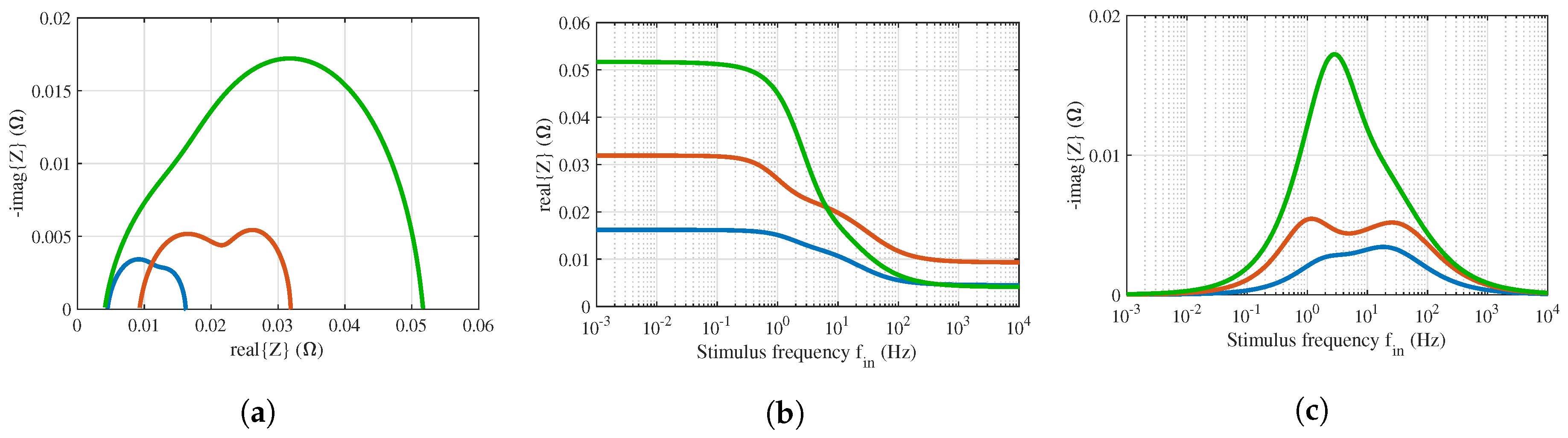
Looking at the real and imaginary parts of the Fouquet impedance (Figure 2), three frequency ranges where the filter response should be analyzed can be identified. Hereafter, the low frequency range (LF) is defined as $f_{in}<10\mathrm{m}\mathrm{Hz}$, the middle frequency (MF) as $10\mathrm{m}\mathrm{Hz}<f_{in}<500\mathrm{Hz}$, and the high frequency range as $f_{in}>500\mathrm{Hz}$ (HF).

Algorithm 1: Analysis of the identifiability domain

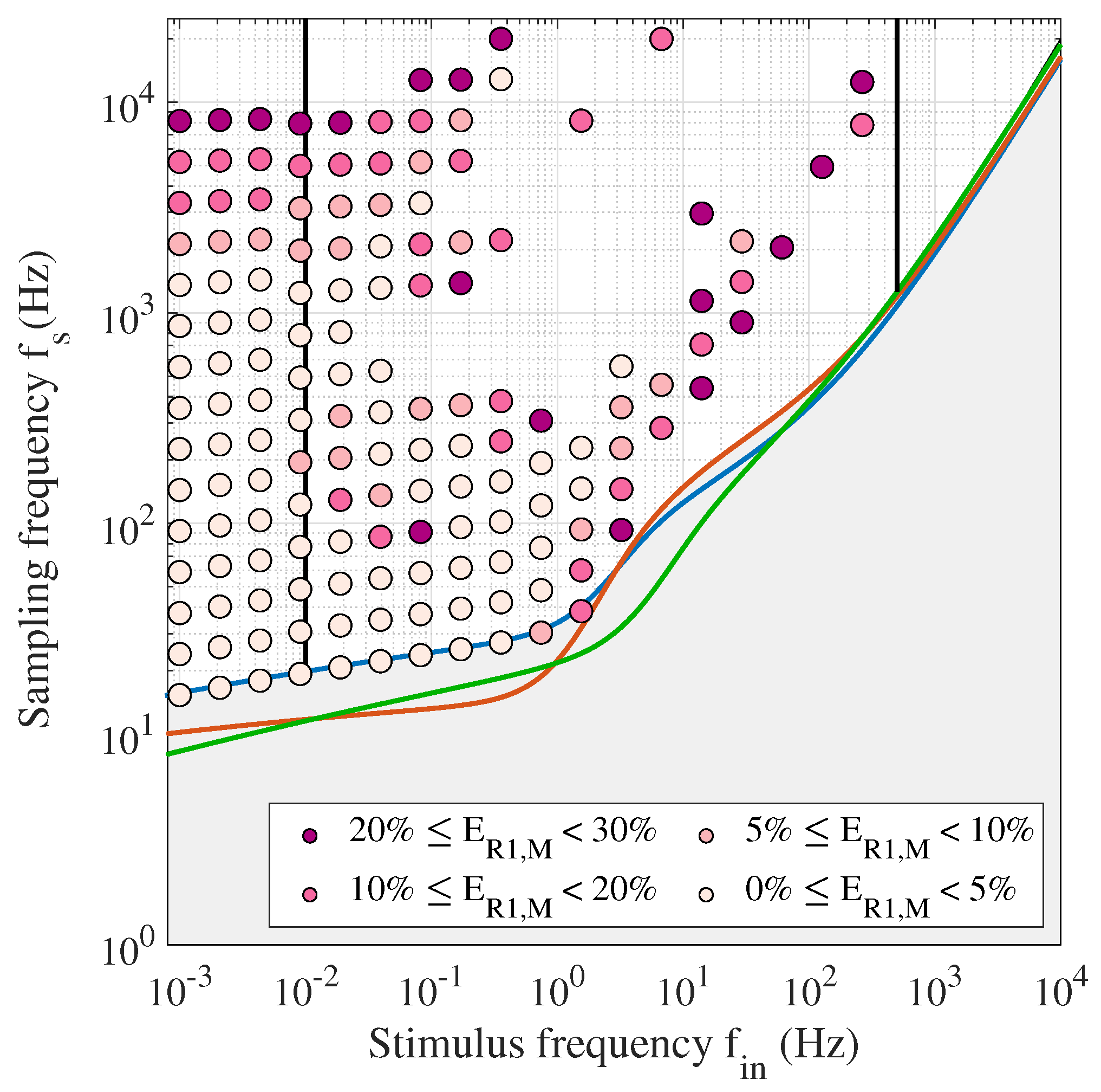
4.1. Parameter Estimation at High Frequency

At HF, the real part of the Fouquet impedance is constant and equal to $R_0$. To identify only this parameter, the estimate for $\alpha$ and $\beta$ were locked at the starting value and ignored by using an extremely small covariance value. This ensures that the DKF will not modify these parameter values to match the output voltage of the RRC model with the voltage measurement.

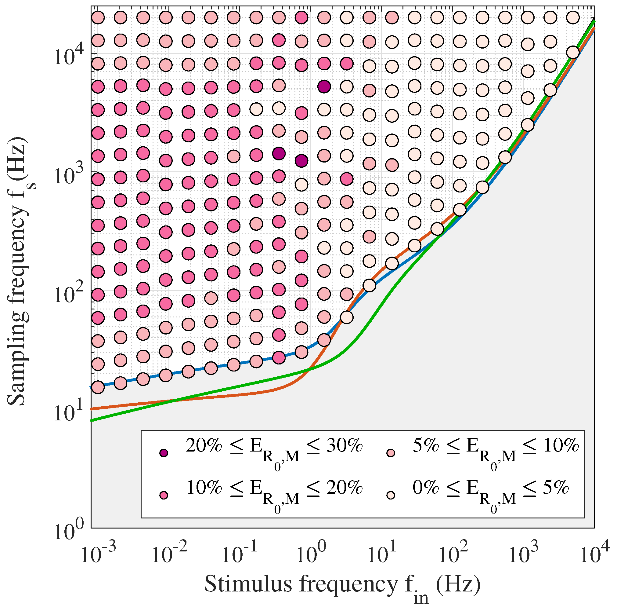
Figure 6 shows the series resistance $R_0$ identification performance in the whole domain by setting ${\gamma }_{R_0}=-7$. In particular, $R_0$ is correctly identified in all the domain areas with $E_{R0,M}<30\%$, with very good performance in HF. In the MF, the error starts to rise, reaching 20–30% in LF. Although the increased error does not affect the region of interest (HF), further insights on the rising trend of the error will be clarified by analyzing the LF region.

4.2. Parameter Estimation at Low Frequency

At LF, the effect of the resistance $R_1$ is important on the real part of the impedance. Around the LF zero-crossing point in the impedance plot (Figure 2a), the impedance tends to be real and equal to $R_0+R_1$. In this neighborhood, the effect of the capacitance $C_1$ is poor. Hence, the parameter to be further estimated at LF is mainly $R_1$, since $R_0$ has already been estimated at HF.

To achieve this result, it is worth maximizing the part of the domain where $E_{R_1,M}<30\%$. This will be done by changing the parameter covariances and evaluating the percentage of the domain in which the error goes below the indicated threshold. In particular, both the total domain area and the LF one are considered

Table 3. Domain area where $E_{R_1,M}<30\%$.

Covariance Vector		Domain Area
${\mathit{\gamma }}_{\mathit{\alpha }}$	${\mathit{\gamma }}_{\mathit{\beta }}$	(% of LF Region)	(% of Total Domain)
−7	−6	88.06	51.48
−7	−7	88.06	52.22
−7	−8	88.06	52.61
−7	−9	86.57	56.32

.

The best performance is achieved by tuning the covariance vector as ${\gamma }_{\alpha }=-7$ and ${\gamma }_{\beta }=-8$, since this configuration allows maximizing of both the areas. In these tests, the values of $R_0$ are locked at the previously identified value.

In these cases, in an area of about 88% of the domain, the identification of the parameter $R_1$ is feasible. Figure 7 shows in details the area for the set with ${\gamma }_{\alpha }=-7$ and ${\gamma }_{\beta }=-8$. A wide area, up to $f_s=$ 1 $\mathrm{k}$$\mathrm{Hz}$ allows us to identify the parameter. Similar areas of the domain are obtained for ${\gamma }_{\beta }$ ranging from $-12$ and $-10$, meaning that an accurate tuning of the covariance vector is not required at LF.

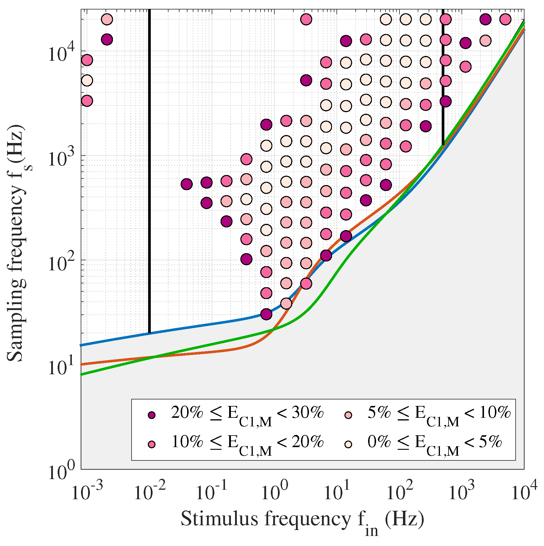
4.3. Parameter Estimation at Middle Frequency

In the MF range (Figure 2a), the contribution on the impedance spectrum comes both from the real and the imaginary parts. Thus, the information on the FC state has to be extracted by both $R_1$ and $C_1$, which need to be estimated. To evaluate the filter performance, $E_M$, i.e., the maximum error over both $R_1$ and $C_1$, is considered and the results are reported in

Table 4. Domain area where $E_M<30\%$.

Covariance Vector		Domain Area
${\mathit{\gamma }}_{\mathit{\alpha }}$	${\mathit{\gamma }}_{\mathit{\beta }}$	(% of MF Region)	(% of Total Domain)
−7	−10	27.02	18.82
−7	−11	40.02	28.78
−7	−12	39.45	26.94
−7	−13	35.13	23.99
−7	−14	27.56	19.56
−7	−15	27.02	12.18

.

This first analysis suggests a further investigation of the covariance sets, choosing ${\gamma }_{\beta }=\{-11,-12,-13\}$. In these cases, the identification is more critical than in HF or LF. The identification of parameters is well achieved in an area of about 35–40% of the MF domain, correctly identifying both parameters. Figure 8 shows the distribution of the successful tests on the $f_s-f_{in}$ plane. In this case, the set with ${\gamma }_{\beta }=-13$ (Figure 8c), despite the narrower area produced, is the most suitable for the identification up to $f_{in}=0.5\mathrm{Hz}$. From this value down to $10\mathrm{m}\mathrm{Hz}$, the covariance ${\sigma }_{\beta }^2$ must be increased to achieve a good estimation performance (Figure 8a,b). This issue will be discussed further in the next Section.

For all the analyzed covariance sets, it is worth noticing the discontinuity of the $E_M$ indicator in the upper part of the $f_s-f_{in}$ plane, where one or both parameters are wrongly estimated. In order to retrieve a deep understanding of the filter response, and to understand whether the estimation of one parameter is more critical than the other one, it is worth inspecting the maximum errors $E_{C_1,M}$ and $E_{R_1,M}$. As an example, the estimate results obtained with the set ${\gamma }_{\alpha }=-7$, ${\gamma }_{\beta }=-13$ are considered. Figure 9 shows the maximum error on the parameter $C_1$, $E_{C_1,M}$. Comparing this figure with Figure 8c, the area is wider, and, obviously, includes the one produced by $E_M$ (Figure 8c). It follows that, at high sampling frequencies, the discontinuity of $E_M$ is mainly due to high errors in the estimate of $R_1$. Here, an increase of the sampling frequency does not lead to any benefit for the parameter identification.

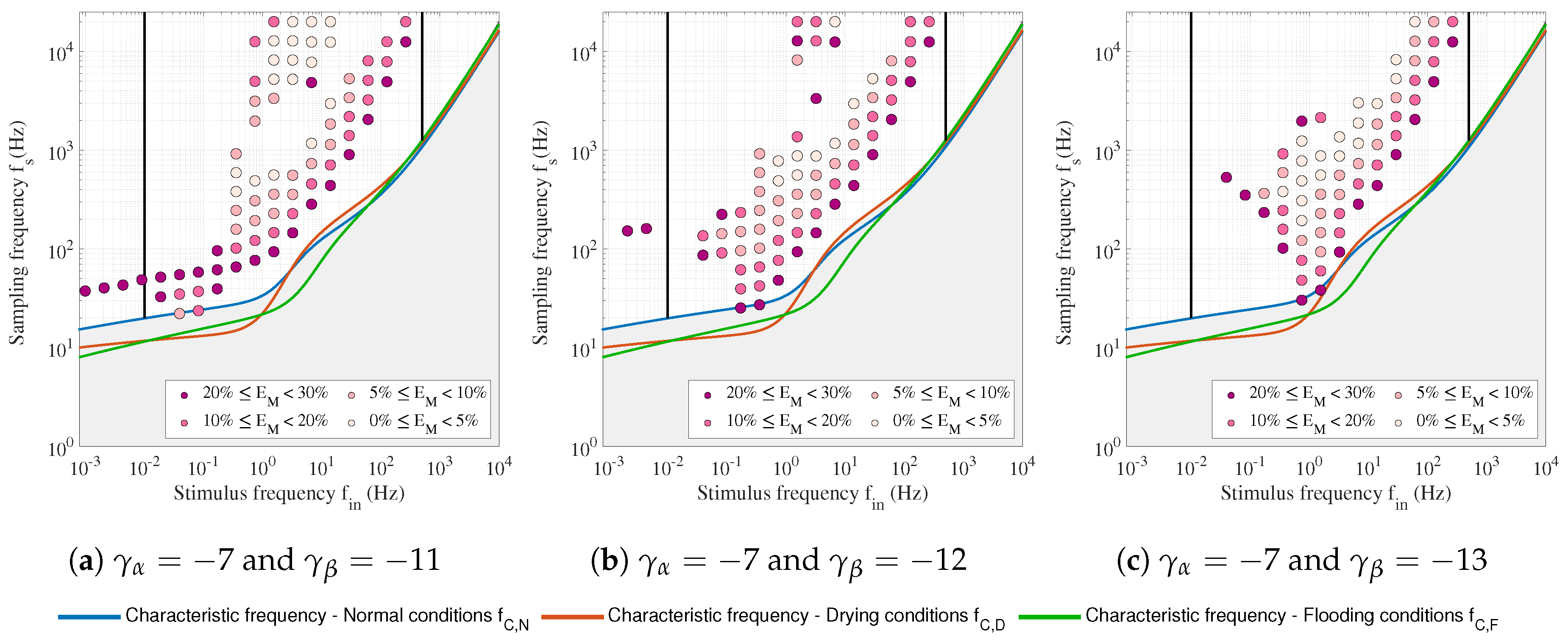
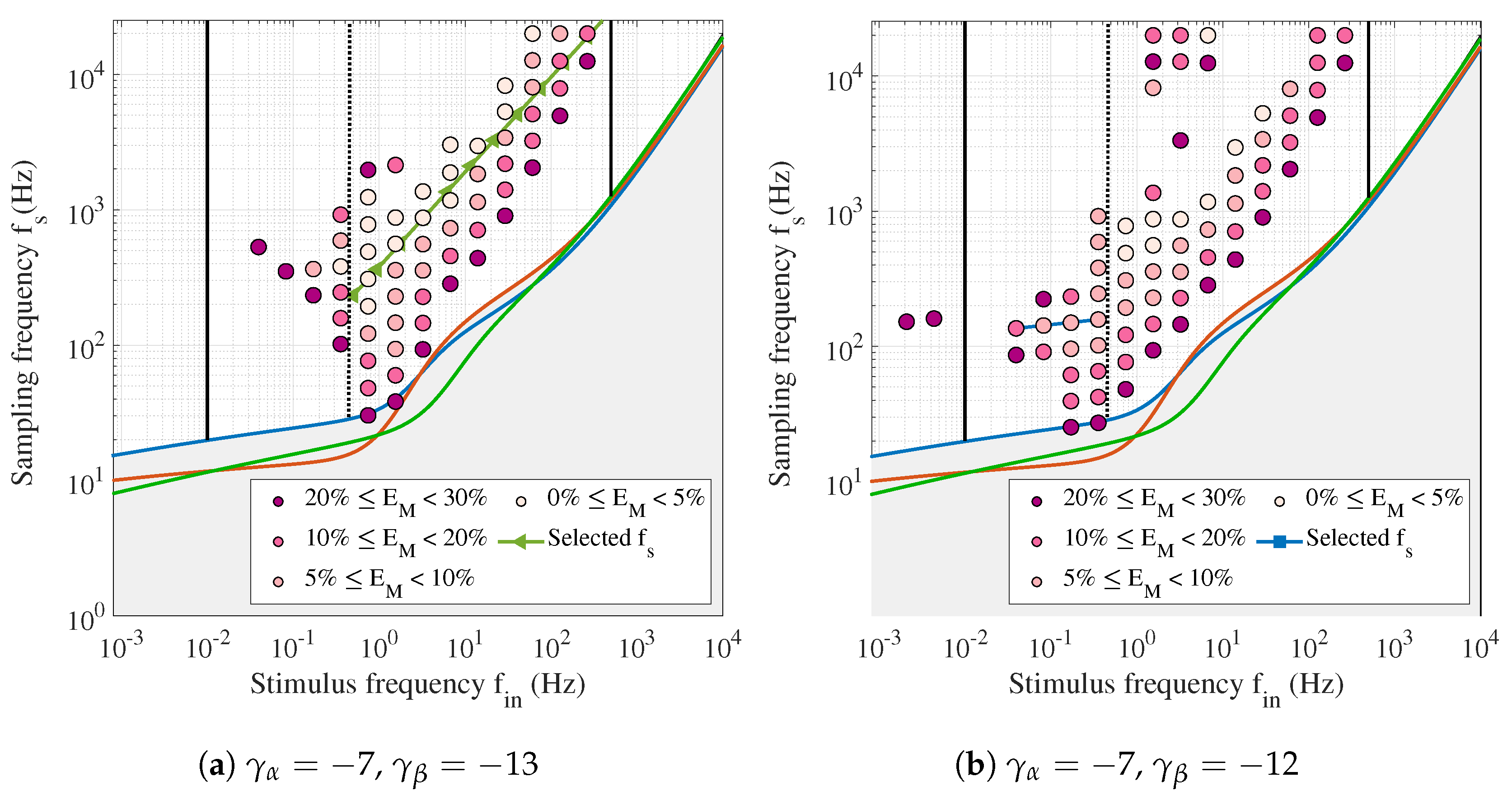
4.4. Sampling Frequency and Covariance Adaptivity

Within the MF interval, the identification remains critical in the lowest part of the spectrum. Here, the identification can be improved by adjusting the covariance to the sampling frequency. From a graphical point of view, this approach allows to close the impedance curve towards the real axis.

Figure 10 summarizes the results obtained by adjusting the covariance vector according to the sampling frequency. At $0.5$ $\mathrm{Hz}$, the sampling frequency profile changes, and this is remarked with a dashed line. Figure 10c shows that more than 80% of the FC spectrum can be identified with a single covariance set, provided that $f_s$ and $f_{in}$ are linked as shown by the green curve of figure Figure 11a. The identified impedance, and the related parameters $R_1$ and $C_1$, are marked with diamonds in all cases (Figure 10).

In the lowest part of the MF, below $0.5$ $\mathrm{Hz}$, the covariance was increased and $f_s$ adjusted as shown in Figure 11b. It is worth observing that the optimal $f_s$ scales proportionally with $f_c$ and an increase in the covariance value of the parameter $\beta$ has to follow. Square markers in Figure 10 highlight the few points earned with this approach.

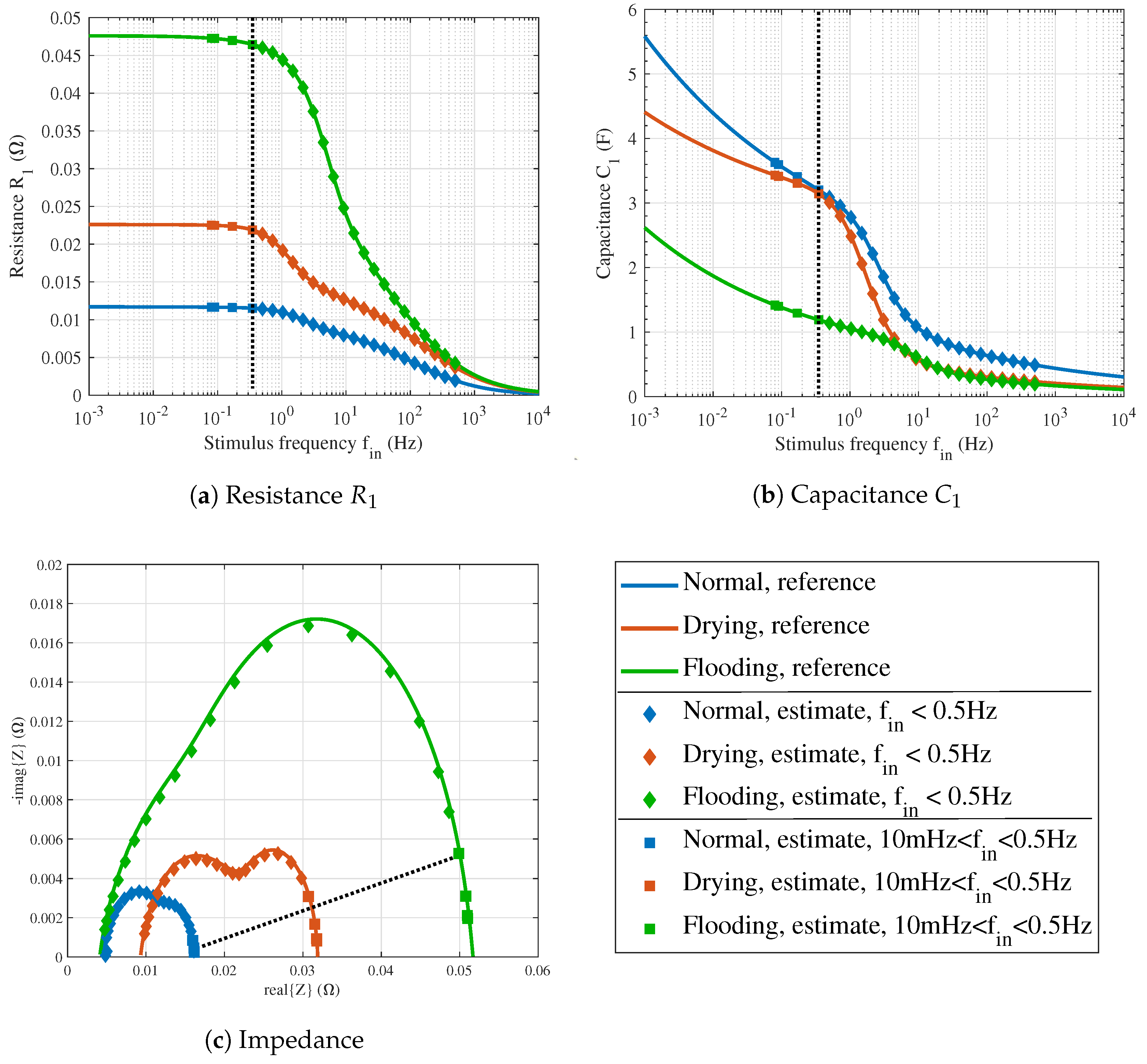
Figure 10c allows one to understand the effect of faults on the impedance plot, while Figure 10a and Figure 10b illustrate the corresponding impact of the fault conditions on the first-order model parameters. An increment of the resistance $R_1$ with respect to normal condition is related to a possible water management fault. This increment is higher at low frequency, but it is detectable since the beginning of the considered EIS test, i.e., at high frequency. Its magnitude, in correspondence of a valuable reduction of capacitance, allows one to distinguish between drying and flooding conditions. In addition to the $R_1$-$C_1$ branch results, the increase of the resistance $R_0$ also helps in detecting the drying condition.

5. Parametric Identification from Experimental EIS Data

The previously discussed results were obtained by following a model-driven procedure. In particular, the choice of the input frequency ranges to be analyzed as well as the error figures to be considered for each particular frequency region, were derived by observing the real and the imaginary parts of the Fouquet model. For this reason, a further investigation is required in real case tests.

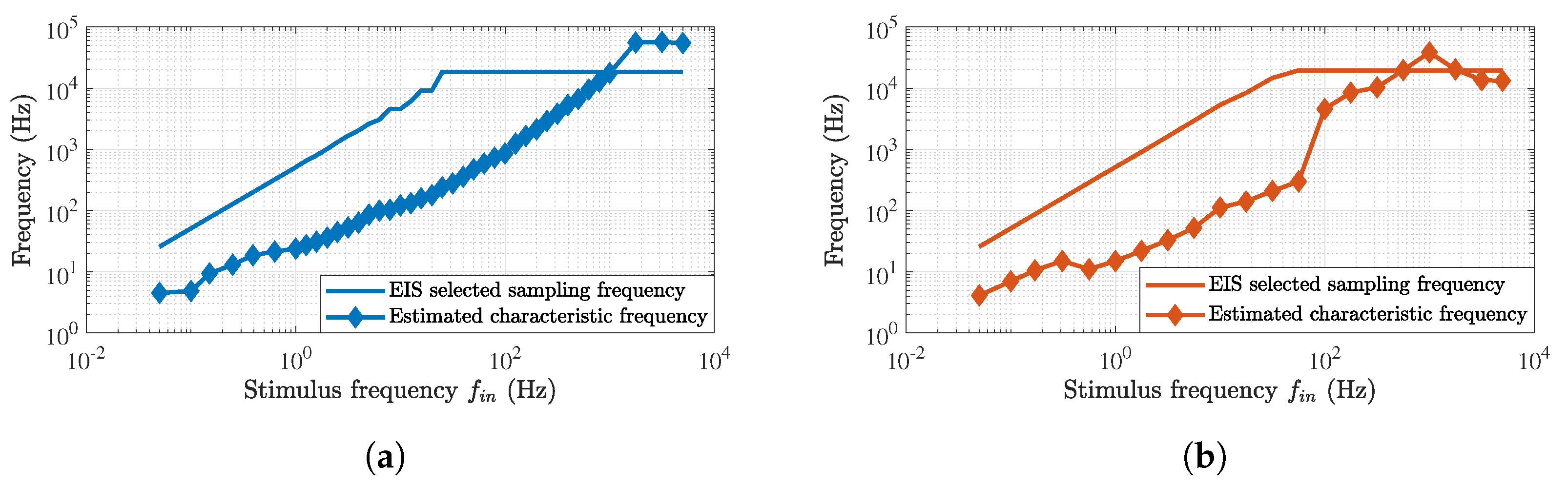
The identification procedure was run on EIS experimental data performed in the framework of the H2020 HEALTH-CODE project [20]. The tests were conducted for a 12-cell PEMFC stack from Ballard Power System. The active cell area of each cell in the stack is 100 cm². The data used hereafter were tested for 35 $\mathrm{A}$ operating point, at a temperature of 57 ${}^{\circ }\mathrm{C}$ both in nominal and in air starvation conditions. The sampling frequency $f_s$, plotted in Figure 12 as a function of $f_{in}$ with solid lines, was determined by the experiment manager.

In this case, no prior characterization of the FC was done, thus, the characteristic frequency $f_c\left(f_{in}\right)$ is unknown. It is worth noticing that, in this case, it is not possible to clearly define the LF, MF, and HF ranges.

The results of the identifications are reported in Figure 12 and Figure 13 for the nominal and air starvation conditions. The markers are the results produced by the DKF-identified model. These results were obtained by identifying $R_0$ with ${\gamma }_{R_0}=-7$, while the other parameters were locked at their initial value. Then, on the basis of the estimate of $R_0$, the remaining parameters were identified by setting ${\gamma }_{\alpha }=-5$ and ${\gamma }_{\beta }=-7$.

In Figure 12, the estimated characteristic frequency ${\widehat{f}}_c$ is plotted with markers. Most of the markers lie below $f_s$, thus indicating identifiability. Some markers, especially those at very high frequency, lie above $f_s$, or very close. In this case, obviously, an accurate identification is not guaranteed.

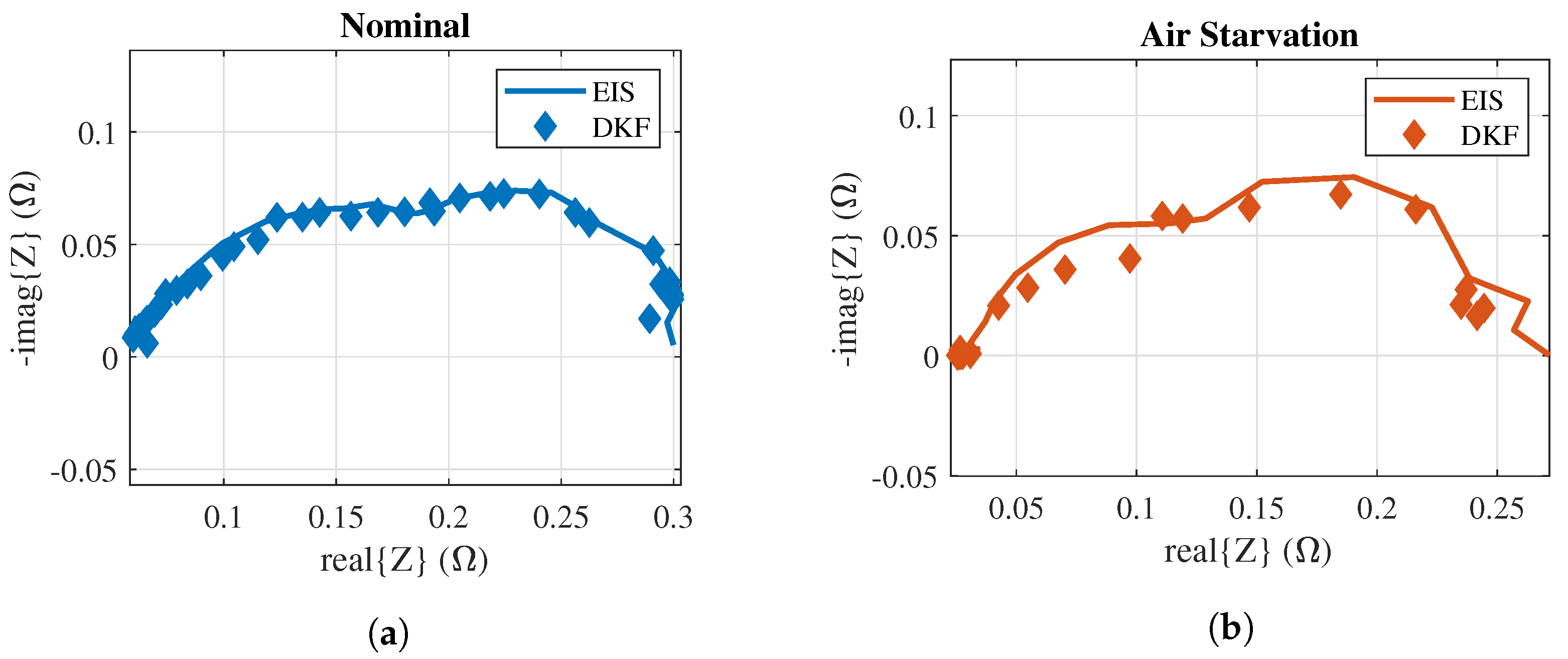
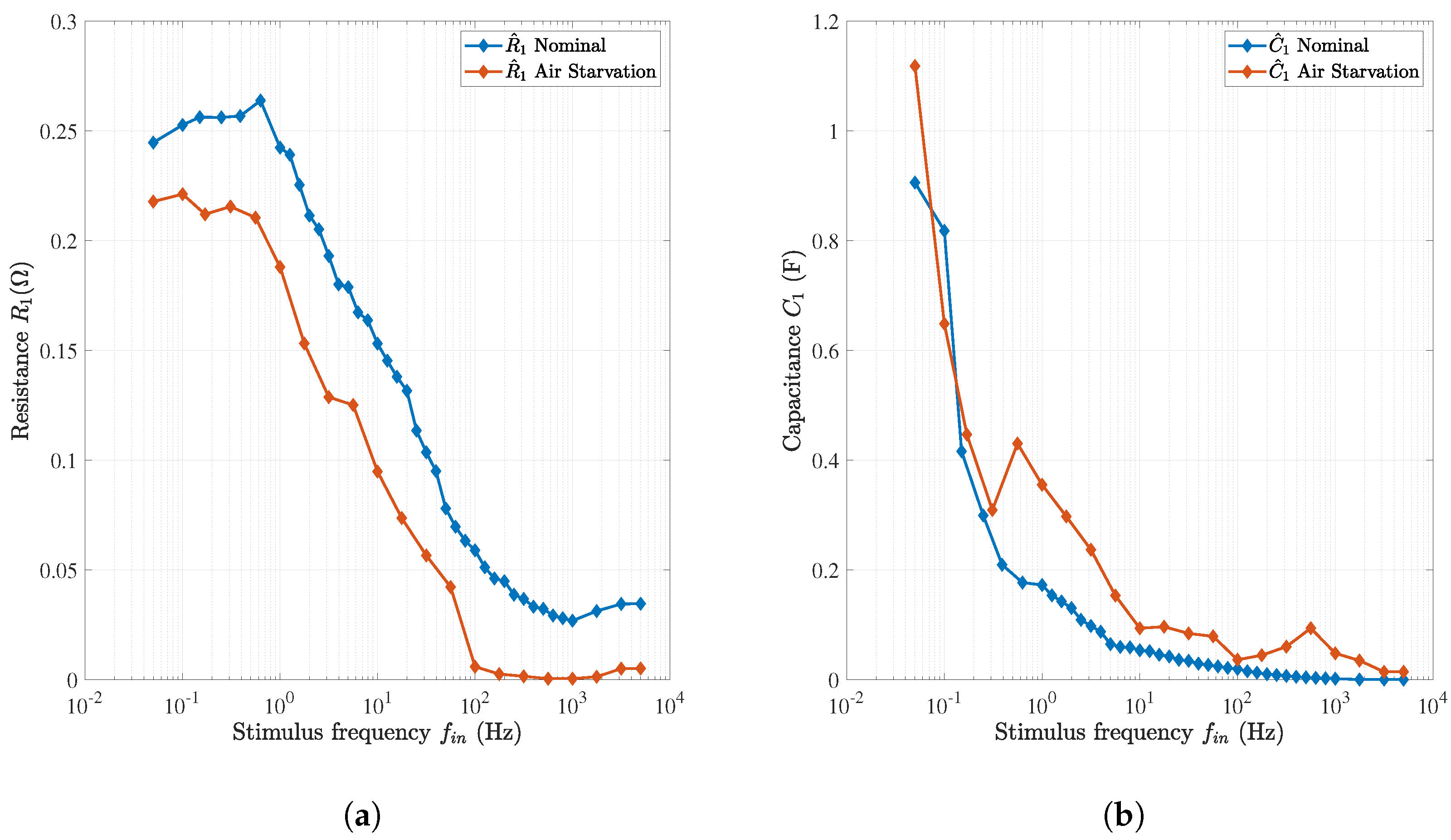
Figure 13 shows the impedance plots. The solid line represents the impedance computed by means of the EIS-based analysis of the voltage and current signals (e.g., FFT). The nominal impedance, in Figure 13a, is reproduced with high fidelity by the DKF approach. In Figure 13b, the less accurate reconstruction of the air starvation spectrum could be ascribed to less-clean time-domain data. Despite this, Figure 14 shows that a valuable deviation of $R_1$ and $C_1$ is observed with respect to the nominal condition. In particular, a decrease of the resistance $R_1$ in conjunction with the decrease of the resistance $R_0$ is observed. These deviations allow, in perspective, the detection of this fault.

It is worth remarking that, in this experiment, $f_s$ is not optimized for the DKF identification. A higher sampling frequency would have given a more accurate result, especially at LF, where $f_s$ should have been adapted as shown in Section 4.4. The identified parameters, in particular, ${\widehat{C}}_1$ in Figure 14b and $f_c$ in Figure 12, are clearly affected by a lack of fidelity at LF, where an unexpected sign-change of the slope occurs.

Similar considerations hold for HF, where a higher $f_s$ would have led the system into the identifiability.

However, when $R_0$ is estimated in the same frequency range, the result is consistent with the left-side real axis intersect of the EIS spectrum.

6. Conclusions

A performance analysis of the Dual Kalman Filter identification capabilities in Electrochemical Impedance Spectroscopy tests was proposed for polymer electrolyte membrane fuel cells. In simulation, the fuel cell behavior is replaced by the Fouquet model, and the filter sequentially identifies the frequency-varying parameters of a simple first-order RC model. The main factors influencing the filter performance are successfully correlated to one another, and the relation between the sampling frequency $f_s$, the characteristic frequency $f_c$, the input signal frequency $f_{in}$, and the initial covariance matrix of the filter is analyzed through a numerical study. The relationship is graphically represented to allow an easy a priori tuning of the filter to be done offline before using the filter in online applications. This allows for retrieval of the best sampling frequency offline and, after, to deploy the Dual Kalman Filter for the online tracking of the parameters in spectroscopy tests. Considering the simplicity and the low computational burden achieved, such an approach constitutes a supporting tool to the frequency-based fault detection that can be implemented onto low-cost embedded devices.

As a future perspective, the proposed approach could be extended to other kinds of fuel cell systems, such as to solid oxide fuel cells under impedance spectroscopy tests, even if the analysis has to be renewed considering two main changes. First, an extension of the analyzed frequency range towards higher frequencies (few tens of kilohertz) could be required to see a whole impedance arc in an impedance plot. Additionally, the characteristic frequency curves might change their shape with respect to the case considered in this paper. This is a worthy matter for further work.