Research on Short-Term Load Prediction Based on Seq2seq Model

Abstract

Electricity load prediction is the primary basis on which power-related departments to make logical and effective generation plans and scientific scheduling plans for the most effective power utilization. The perpetual evolution of deep learning has recommended advanced and innovative concepts for short-term load prediction. Taking into consideration the time and nonlinear characteristics of power system load data and further considering the impact of historical and future information on the current state, this paper proposes a Seq2seq short-term load prediction model based on a long short-term memory network (LSTM). Firstly, the periodic fluctuation characteristics of users’ load data are analyzed, establishing a correlation of the load data so as to determine the model’s order in the time series. Secondly, the specifications of the Seq2seq model are given preference and a coalescence of the Residual mechanism (Residual) and the two Attention mechanisms (Attention) is developed. Then, comparing the predictive performance of the model under different types of Attention mechanism, this paper finally adopts the Seq2seq short-term load prediction model of Residual LSTM and the Bahdanau Attention mechanism. Eventually, the prediction model obtains better results when merging the actual power system load data of a certain place. In order to validate the developed model, the Seq2seq was compared with recurrent neural network (RNN), LSTM, and gated recurrent unit (GRU) algorithms. Last but not least, the performance indices were calculated. when training and testing the model with power system load data, it was noted that the root mean square error (RMSE) of Seq2seq was decreased by 6.61%, 16.95%, and 7.80% compared with RNN, LSTM, and GRU, respectively. In addition, a supplementary case study was carried out using data for a small power system considering different weather conditions and user behaviors in order to confirm the applicability and stability of the proposed model. The Seq2seq model for short-term load prediction can be reported to demonstrate superiority in all areas, exhibiting better prediction and stable performance.

1. Introduction

Short-term load forecasting has an important impact on major decisions, such as the day-to-day operation of the power grid and dispatch planning [1]. Many scholars have carried out numerous studies on power system load prediction, among which the traditional prediction methods include the time series method [2], the regression analysis method [3,4], trend extrapolation [5], etc. The implementation principle of these methods is simple, fast operation speeds that are suitable for processing data characteristics of a single and small data set. However, despite their nonlinear characteristics, large data volumes, lack of robustness, and poor adaptability, modern load prediction methods mainly include gray mathematical theory [6,7], fuzzy prediction method [8], neural network method [9,10], and so on. In recent years, artificial intelligence has come to be widely used in image processing, speech recognition, power systems [11], and other fields. In the smart grid, artificial intelligence is widely used in power generation, transmission, power distribution, and the power market, while on the power side, accurate load prediction is carried out using the artificial intelligence algorithm [12], which effectively reduces the cost of power generation, making reasonable power generation plans for the power system. Through the real-time prediction of user-side power consumption, the power grid dispatch work is carried out in a punctual and appropriate manner, so as to maintain the safe and stable operation of the power grid.

Deep learning algorithms exhibit a good ability to extract data characteristics when processing large amounts of power data, and power system load prediction is designed to extract typical features from complex and variable historical load data, so as to make accurate load predictions. The power system load data is typical time-series data. Therefore, the use of deep learning algorithms to process the load data achieves better results. The literature has put forward a time series decomposition model [13], which effectively reflects the factors that affect load prediction in order to achieve the accurate prediction of load data; however, it is easy to ignore the correlation between time periods, and the load prediction of some time periods is significantly biased. The paper proposes a time series prediction method based on the lifting of wavelets [14], which predicts the electricity consumption in residential areas by means of denoising the historical load data, exhibiting a stronger nonlinear feature extraction ability than the time series model deep learning algorithm. Studying the factors influencing load prediction, a load prediction model based on artificial neural network (ANN) was developed [15]; however, the model is easily caught in local extreme values and lacks the modeling of time factors during ANN training. By using an ant colony optimization algorithm to optimize the recurrent neural network (RNN) prediction model, the prediction accuracy of traditional RNN is improved [16], there is a problem of gradient disappearance and long-term dependence. To improve the accuracy of traditional RNN prediction, the problems of gradient disappearance and long-term dependence need to be solved, and the authors adopt the long-term and short-term memory network (LSTM) prediction model method, combined with the real-time electricity load data, in order to solve the problems of gradient disappearance and long-term dependence [17], but lacks consideration of the influence of historical information and future information on the current state. Self-encoders are unsupervised deep learning models with stronger feature extraction abilities, and a stack-based self-encoder prediction model was introduced that extracts the characteristics of the input data in a comprehensive way [18], which has strong prediction accuracy and generalization ability.

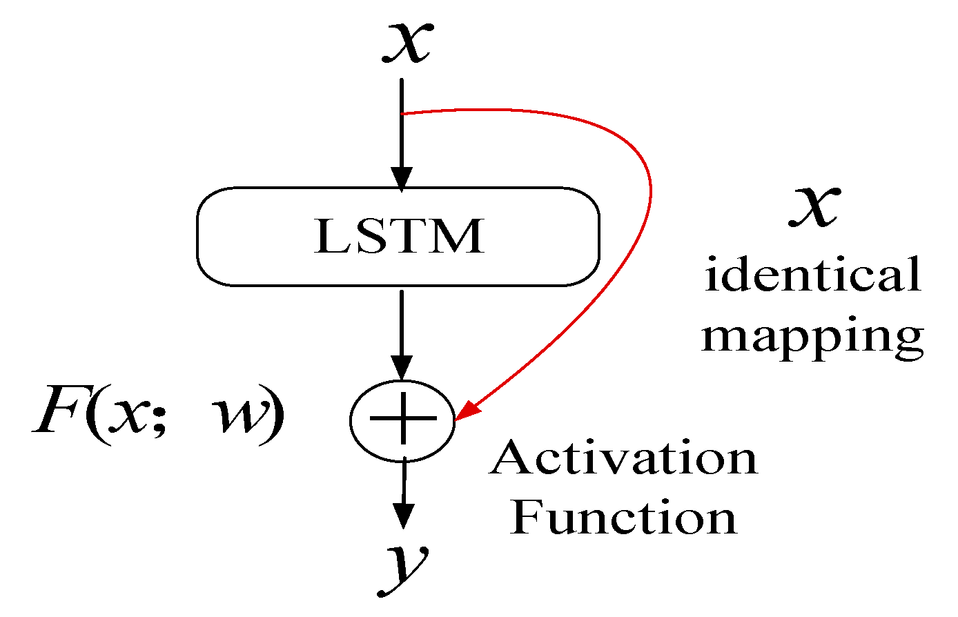
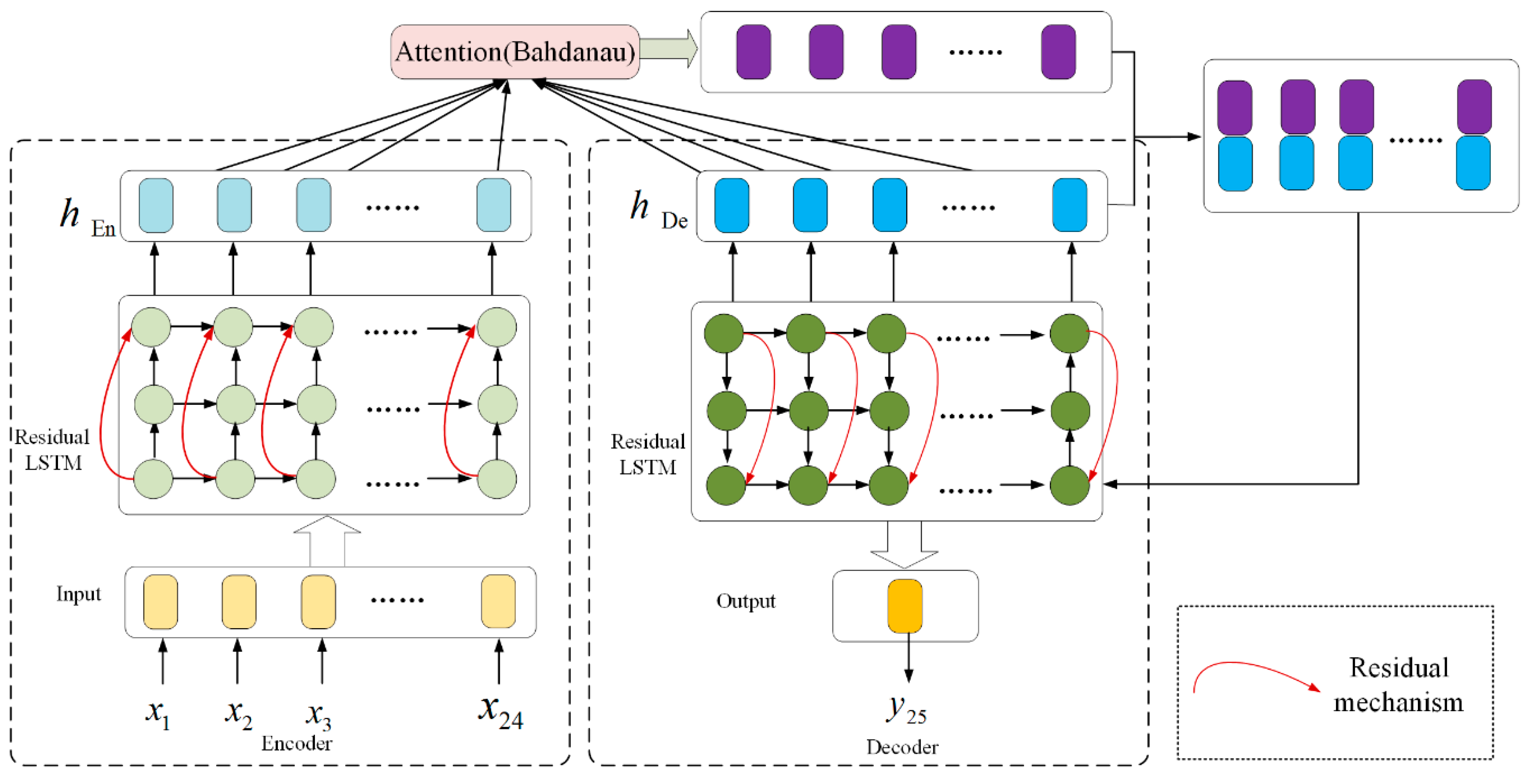
Based on our research into the above literature, and by observing the shortcomings of the above prediction methods, this paper proposes a short-term load prediction model of the Seq2seq codec based on LSTM and improves the performance of the multi-layer LSTM network by adopting the Residual mechanism. The introduction of the Attention mechanism into the decoding process achieves selective feature extraction of load prediction data, improves the correlation of input and output data, improves the accuracy of model prediction, and ultimately, comparison with other prediction methods indicates that the method proposed in this paper has better prediction effect.

2. Motivation and Problem Statement

At present, although the power industry is vigorously developing huge energy storage devices, because of the special nature of electricity, it is still difficult to implement large-scale storage at this stage. The prediction of electricity load is carried out so as to reasonably plan power generation and reduce power wastage, with each increase in load forecast accuracy of 1% saving about 0.1% to 0.3% in energy costs [19]. With the large-scale grid interconnection of new loads, such as renewable energy and flexible loads (such as electric vehicles), the components of user-involved load consumption are growing more complex every day. The uncertainty and nonlinearity of the electricity load are gradually increasing, and the relationship between the demand of the source and the load-side consumption is maintained, which is consistently increasing the accuracy of load prediction. Improving the accuracy of user-side load prediction plays an important role in power grid power planning and power scheduling [20].

Increasing the load forecasting level saves coal and reduces power generation costs, helping to formulate reasonable power supply construction plans, which will then help in increasing the economic benefits of power systems and society [21,22].

A key area of investigation in power load forecasting is the means by which existing historical data can be used to establish suitable forecasting models to predict the load at a future time or in a given time period. Therefore, the reliability of historical load data and the choice of the predictive model are the main factors influencing precision. As the nonlinearity and uncertainty of the power dataset increase, the difficulty of obtaining accurate load forecasting results increases. The accuracy of the prediction results has always been a process that needs to be continuously improved, from the traditional regression prediction method to the current deep learning algorithm [23,24]. The prediction method is improving constantly. The deep learning algorithm has the characteristics of information memory, self-learning, optimization calculation, etc. It also has strong computing power, complex mapping ability, and various intelligent processing capabilities [25].

3. Seq2seq Codec

The Seq2seq model is Google’s mainstream machine translation architecture. It was originally applied in the field of machine translation [26], which is suitable for sequence-to-sequence applications. Seq2seq consists of two parts, an encoder and a decoder, which effectively extracts the features of the input data. The users’ power system load data has typical time-series characteristics. Load prediction using the Seq2seq model achieves better results. Therefore, this paper proposes using the Seq2seq model in order to calculate the electricity consumption of residents.

3.1. LSTM

The RNN has many advantages with respect to the processing of sequence data, but it is more prone to gradient disappearance and gradient explosion. LSTM is an algorithm developed on the basis of RNN to solve the gradient vanishing problems faced by RNN, and has an advantage over RNN with respect to handling complex long-term data.

Figure 1 shows the typical structure of LSTM, consisting of three main gate structures: forget gate, input gate, and output gate. Here, $x_t$ denotes the input data, $h_t$ denotes the hidden state, $c_t$ is defined as cell state, $f_t$ denotes the output state of the updated forgotten gate, $i_t$ and $c$ are the updated input gate and output state respectively, and $o_t$ is the output state of the updated output gate. The calculated equations for each state are as follows [27]:

$$f_t=\sigma (W_f{h}_{t-1}+V_f{x}_t+b_f)$$

(1)

$$i_t=\sigma (W_i{h}_{t-1}+V_i{x}_t+b_i)$$

(2)

$${\tilde{c}}_t=\tanh (W_{\tilde{c}}{h}_{t-1}+V_{\tilde{c}}{x}_t+b_{\tilde{c}})$$

(3)

$$c_t=c_{t-1}\cdot f_t+i_t\cdot {\tilde{c}}_t$$

(4)

$$o_t=\sigma \left(W_o\left[h_{t-1},x_t\right]+b_o\right)$$

(5)

$$r_t=o_t\times \tanh (c_t)$$

(6)

$$h_t=W_p\cdot r_t$$

(7)

where, $W$ and $V$ correspond to the weight matrix, $b$ is the bias coefficient, $\sigma$ and $\tanh$ are the activation function.

3.2. Seq2seq Codec Principle

Seq2seq places no limit on the length of the input sequence or the output sequence. Recently, the Seq2seq model has been widely used in the field of machine translation [26,28,29]. The structure of Seq2seq is shown in Figure 2.

As shown in Figure 2, the Seq2seq codec consists of an encoder, an intermediate vector $c$, and a decoder. Codecs are typically multi-layer RNN or LSTM structures, wherein the intermediate vector $c$ incorporates the sequence of $x_1,x_2\dots x_m$ encoding information. For time $t$, the output of the previous moment $y_{t-1}$, the hidden layer state of the previous moment $s_{t-1}$, and $c$ are fed as input into the decoder. Finally, the decoder’s hidden layer state $s_t$ is obtained, which predicts the output value.

4. A Short-Term Load Prediction Model Based on Seq2seq Codec Structure

4.1. Attention Mechanism

In this paper, the Seq2seq codec structure is used as the load prediction model, in which the LSTM structure is used by the encoder and the decoder. The encoding end outputs the variable-length sequence as a fixed-length sequence. As the input sequence is lengthy, it is difficult for the decoding end to obtain effective information. Therefore, the output of the LSTM encoder to the input sequence is preserved by introducing the Attention mechanism. Then, the model is trained to selectively learn these inputs, associating the output sequence with the model outputs. In turn, highly correlated useful features are extracted with the output sequence. The main equations that describe the Seq2seq codec structure model are as follows:

The input and output sequences of the model are recorded as x and y:

$$x=(x_1,x_2\cdots x_m)$$

(8)

$$y=(y_1,y_2\cdots y_n)$$

(9)

The hidden layer status of the encoder section is recorded as $h_t$:

$$h_t={\mathrm{LSTM}}_{\mathrm{enc}}(x_t,h_{t-1})$$

(10)

In the decoding process, the Attention mechanism is introduced, comparing the two attention mechanisms: Bahdanau Attention [30] and Luong Attention [31]. These two attention mechanisms are similar in structure, but their alignment functions are different in the decoding process.

(1)

Bahdanau Attention: During decoding, the first step is to generate the semantic vector for particular time:

$$c_t={\displaystyle \sum _{i=1}^T}{\alpha }_{ti}{h}_i$$

(11)

$${\alpha }_{ti}=\frac{\exp \left(e_{ti}\right)}{{\displaystyle {\sum }_{k=1}^T\exp \left(e_{tk}\right)}}$$

(12)

$$e_{ti}=V_a^{\mathrm{T}}\tanh \left(W_a[s_{t-1},h_i]\right)$$

(13)

where $c_t$ is the semantic vector at time t, $e_{ti}$ is the degree of influence of the hidden state $h_i$ of LSTM in the process of encoding, and of the hidden state $s_t$ of LSTM in the process of decoding. ${\alpha }_{ti}$ is a normalized value given by the softmax function. V and W are the weight parameters of the model.

The second step passes the hidden layer information:

$$s_t=\tanh \left(W\left[s_{t-1},y_{t-1},c_t\right]\right)$$

(14)

(2)

Luong Attention: During decoding, the first step is to generate the semantic vector for time t:

$$c_t={\displaystyle \sum _{i=1}^T}{\alpha }_{ti}{h}_i$$

(15)

$${\alpha }_{ti}=\frac{\exp \left(e_{ti}\right)}{{\displaystyle {\sum }_{k=1}^T\exp \left(e_{tk}\right)}}$$

(16)

$$s_t=\tanh \left(W\left[s_{t-1},y_{t-1}\right]\right)$$

(17)

$$e_{ti}=s_t^{\mathrm{T}}{W}_a{h}_i$$

(18)

The second step passes the hidden layer information:

$${\tilde{s}}_t=\tanh \left(W_c\left[s_t,c_t\right]\right)$$

(19)

Unlike the Bahdanau Attention mechanism, Luong Attention computes the initial state of the hidden layer $s_t$ and then the hidden layer state of the decoder ${\tilde{s}}_t$.

During the decoding process, the new weight vector of the decoder LSTM is obtained by the Attention mechanism, and the power system load is predicted using the trained LSTM.

4.2. Residual Mechanism

LSTM has an internal storage unit that enables LSTM to learn time series data for long-term dependence. Compared to RNN, LSTM avoids to some extent the gradient disappearance or gradient explosion problems associated with the increase in training number. However, with the increase in the data volume, the number of LSTM layers and the amount of training data leads to the model being overtrained. Therefore, this paper adopts Residual LSTM [32], modeled on the residual neural network ResNet, which was proposed by Kaiming He [33] to overcome this overtraining problem. Residual LSTM provides an additional low-space shortcut path, which uses the output layer to separate the fast path of space from the fast path of time when training multi-layer LSTM. Residual LSTM uses LSTM’s output projection matrix and output gate to control the spatial information flow, rather than the additional gate network. When the network reaches the optimal state, the network only retains the constant mapping value of the input vector, effectively reducing the network parameters and improving the network performance. A structural diagram of the Residual LSTM is illustrated in Figure 3.

The residual network is calculated by a quick path, and since the identity map is always on, the function output only needs to learn the residual mapping, as shown in Equation (20):

$$y=F\left(x;W\right)+x$$

(20)

where $y$ is the output layer, x is the input layer, $F\left(x;W\right)$ is the mapping, and $W$ is the internal weight parameters of the network. In the absence of the shortcut path, $F\left(x;W\right)$ represents the output $y$ obtained by the input $x$, and when there is a constant map of input x, $F\left(x;W\right)$ only needs to learn the residual mapping $y-x$. When the model training is stable, no new mapping is required, and the network is transmitted directly by constant mapping $F\left(x;W\right)$, thus simplifying the training of deep networks.

There was no change in the Residual LSTM type (1)–(5), and the update changes are as follows:

$$r_t=\tanh \left(c_t\right)$$

(21)

$$m_t=W_p\cdot r_t$$

(22)

$$h_t=o_t\cdot \left(m_t+W_h{x}_t\right)$$

(23)

Here, $W$ is the weight of the model.

4.3. Short-Term Load Forecasting Model and Flowchart

Figure 4 shows the load prediction model used in this paper. First of all, the electricity load data is obtained from the data center, then the data is pre-processed, and finally, a short-term load prediction is made through the intelligent algorithm presented in this paper.

In this paper, the Seq2seq model based on LSTM is used to realize the short-term load prediction model for users, and the specific implementation process is illustrated in Figure 5. Firstly, the raw data is collected and carried out with respect to the residents. Then, the historical electricity load data is passed through data cleaning and pre-processing, using mean value substitution for missing values, etc. The processed data is separated into a training data set and a test data set. The model is trained with the training data, the parameters of LSTM of the Seq2seq model, the Attention mechanism and the Residual mechanism are optimized, and the trained Seq2seq model is implemented by TensorFlow. The preservation and extraction of the model are realized by tf.train Saver, and the effectiveness of the model is verified using the test data set, from which it predicts the short-term user electricity load, and these prediction results are analyzed to determine any shortcomings and to continuously improve the model.

In [34], Niu et al. analyzed the RNN structure using the numerical method of ordinary differential equations, and proposed an ODE theoretical framework to prove the training stability of the LSTM architecture. In [35], the residual neural network (ResNets) composition rules were mapped between hidden variables and the Euler discretization of continuous differential equations, thereby improving the training stability. Thus, the proposed model consists of a residual neural network and an Attention mechanism, showing better stability under a variety of conditions, as described in Section 5.4.

5. Simulation Experiments

5.1. Introduction to the Dataset

This research study was carried out on a personal computer with a single CPU of 2.6 GHz and 8 GB of memory. The simulation process was done using Python 3.6.8, and the TensorFlow deep learning framework developed by Google.

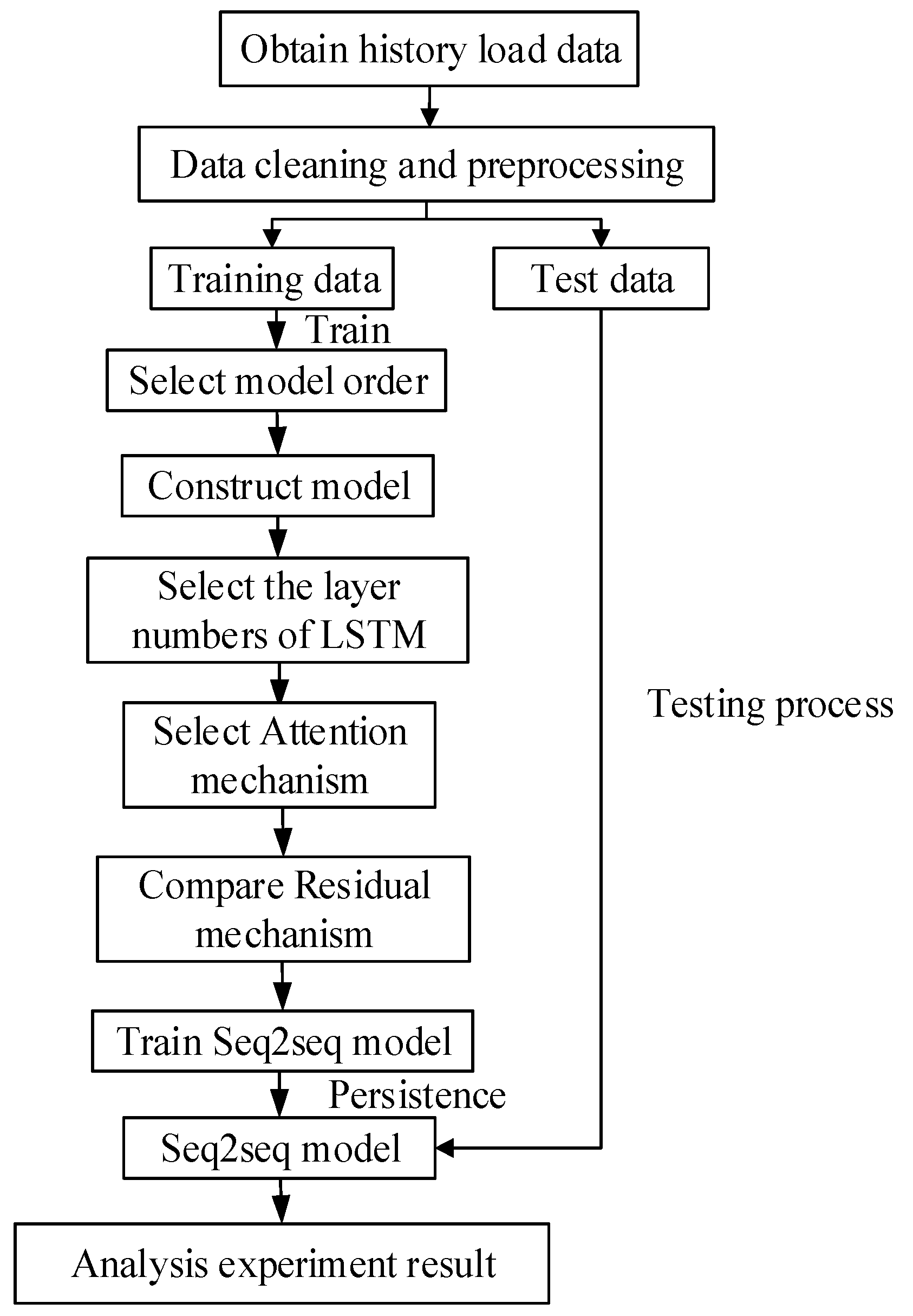
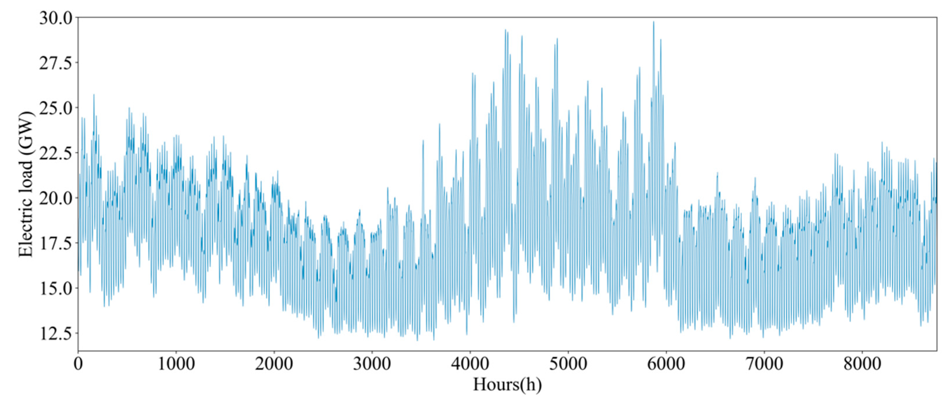
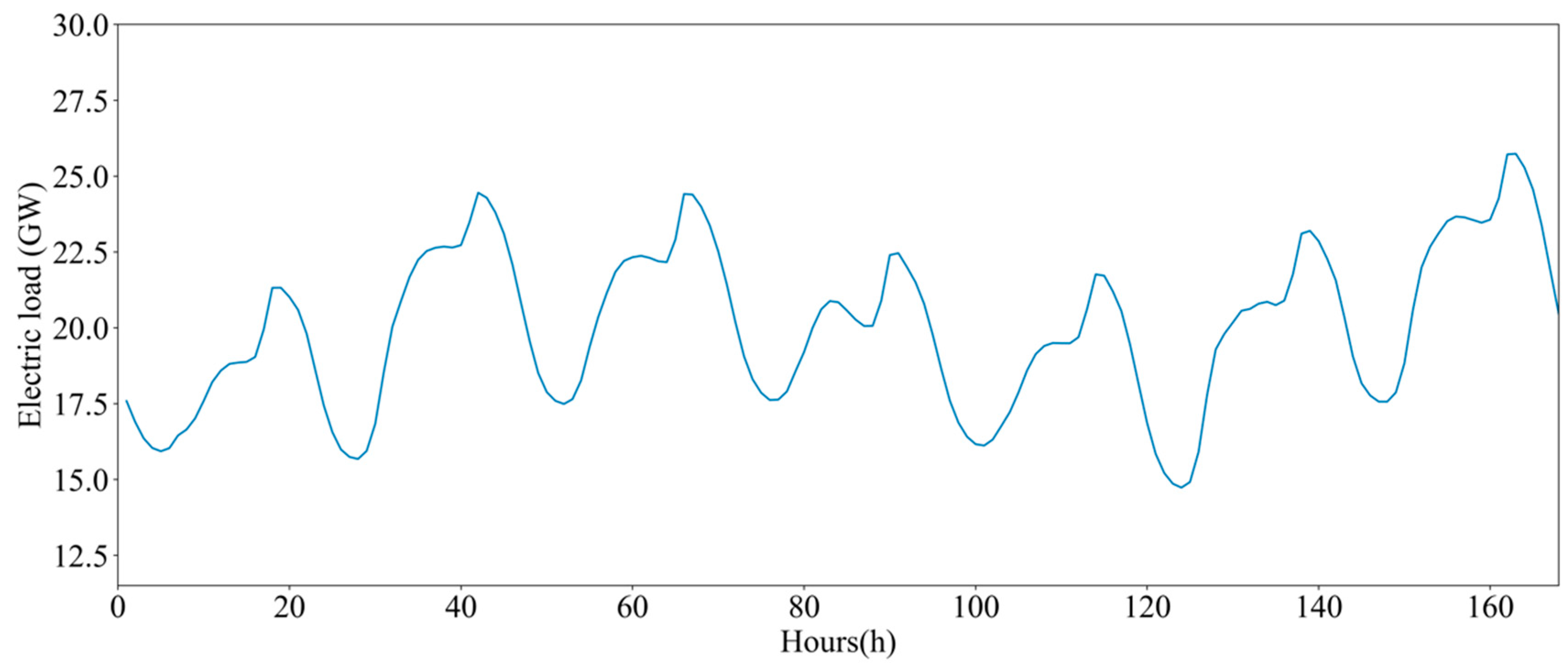
In this paper, the New York State Power history power system load data, published by NYISO Corporation [36], was selected as input for the model training and testing process. Hourly data was selected as a load point, and a total of 8760 load data, of which 80% comprises the training data set and the remaining 20% comprises the test data set. The first 7008 load data were used as a single variable load prediction training data set, and the remaining 1752 load data were used as a single variable load prediction test data set.

Figure 6 clearly shows that the load data fluctuates periodically, wherein the 168-h load data for a week are shown in Figure 7.

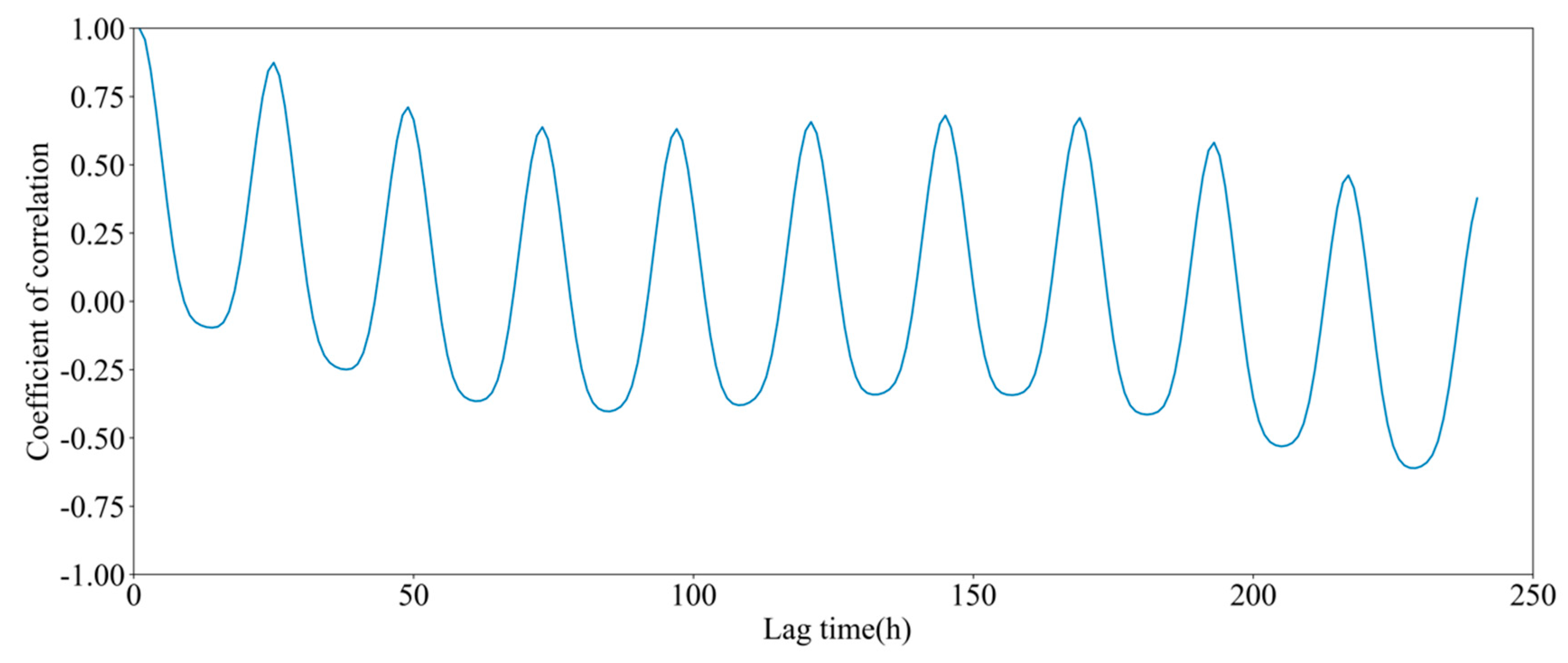
The electricity load is a random process, in the study of random processes, the self-correlation coefficient shows whether the random process is stable and chooses the appropriate model order. Therefore, the self-correlation coefficient of the training data is calculated, as shown in Figure 8.

Figure 7 shows the electricity load in a particular area, showing periodic fluctuations, and Figure 8 shows, with the increase in latency, that the correlation coefficient begins to decrease in the early stage, and with the increase of lag time, when the lag time is 24 h, the maximum peak is 0.87439. Therefore, the selected time series model order is 24, i.e., the historical load data of the first 24 hours of data is used as the characteristic vector rolling prediction. Hence, it is proved that the model is more applicable when using only single-dimensional data to build the model.

5.2. Performance Indices

For the performance evaluation of the proposed model, this paper uses Mean Square Error (MSE), Root Mean Square Error (RMSE), Mean Absolute Error (MAE), and Mean Absolute Percentage Error (MAPE). The measures of error are expressed as follows:

$$\{\begin{array}{l}\mathrm{MSE}=\frac{1}{m}{\displaystyle \sum _{i=1}^m{(y_i-{\widehat{y}}_i)}^2}\\ \mathrm{RMSE}=\sqrt{\frac{1}{m}{\displaystyle \sum _{i=1}^m{(y_i-{\widehat{y}}_i)}^2}}\\ \mathrm{MAE}=\frac{1}{m}{\displaystyle \sum _{i=1}^m\left|y_i-{\widehat{y}}_i\right|}\\ \mathrm{MAPE}=\frac{100\%}{m}{\displaystyle \sum _{i=1}^m|\frac{y_i-{\widehat{y}}_i}{y_i}|}\end{array}$$

(24)

Here, ${\widehat{y}}_i$ represents the true value, $y_i$ represents the predicted value, and $m$ represents the dimension of the data.

The MSE represents the expectation of the difference between the estimated values and the true values. In addition, RMSE is the square root of MSE, describing the magnitude of the errors in terms of making decision making more convenient for users. MAE is the average of the absolute errors between the estimated values and the true values, reflecting the true estimated value error. Moreover, MAPE expresses the percentage error accuracy between error and true values. The lower values of MSE, RMSE, MAE, and MAPE shows better prediction characteristics.

5.3. Seq2seq Preferred Model Parameters

In this paper, the Seq2seq codec structure is used to predict the electricity load, with both encoding and decoding using the LSTM structure, followed by the number of LSTM layers to optimize the number of layers in the model.

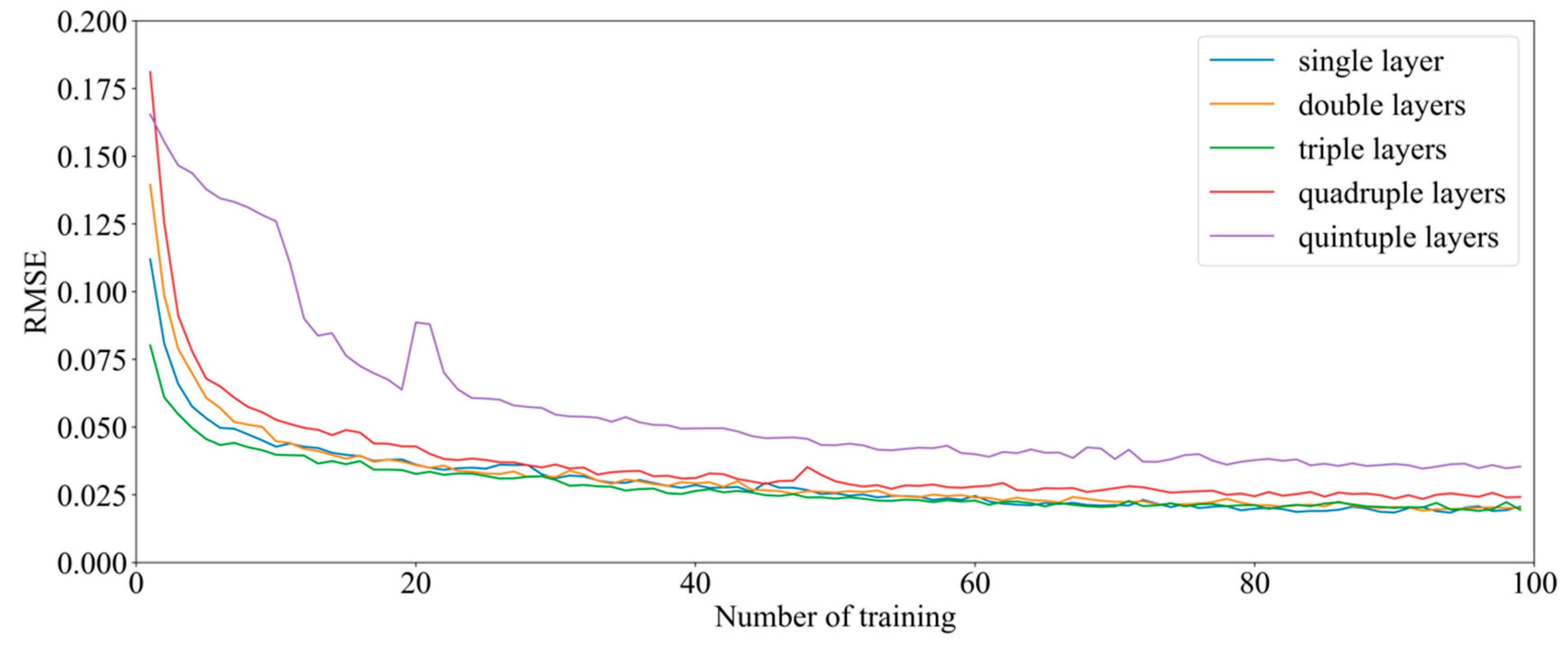
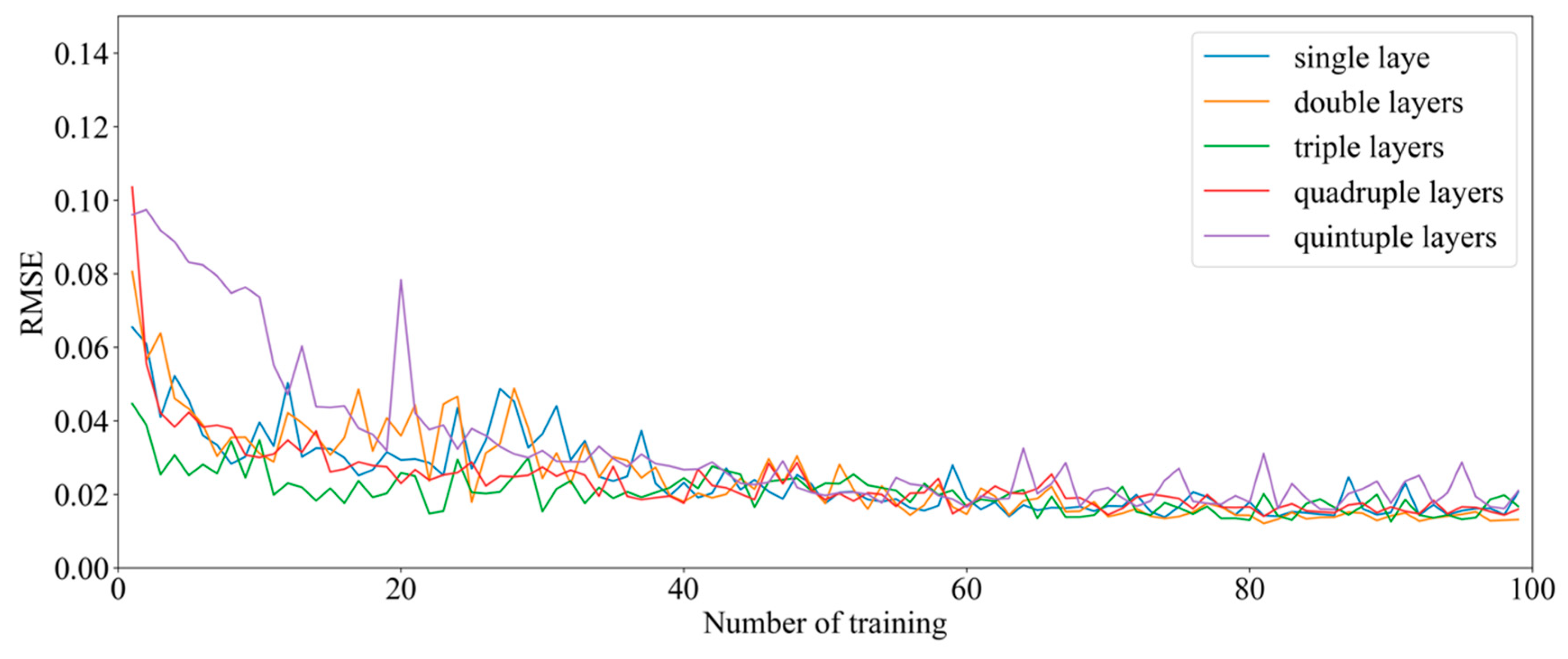
The initial learning rate of the experiment was set to 0.01, the attenuation rate was set to 0.5, the number of hidden layer nodes was set to 100, and after 100 trainings, the training error and test error obtained by the model under the selection of different layers are shown in Figure 9 and Figure 10, respectively.

Figure 8 shows that the training error of using quintuple layered LSTM structure is large, and the test errors after single layer, double layer, and triple layer training are comparatively lower. From Figure 10, the test error of the Seq2seq model with single layer, double layer and quintuple layer LSTM structures are highly volatile. Therefore, the combined comparison of Figure 9 and Figure 10 suggests the selection of the three-tier LSTM structure model, as the error is minimal.

In deep learning, the model learns the “universal law” of all samples from the training sample through training, which tends to cause overfitting and underfitting. By increasing the amount of model training iterations, it is possible to overcome the phenomenon of underfitting. By increasing the data set and introducing the formal approach, it is possible to overcome the overfitting phenomenon. This paper adopts Dropout [37] on this basis of the nerve unit, which is temporarily removed from the network with a probability of 0.5 during training, and the Attention mechanism and Residual mechanism are introduced.

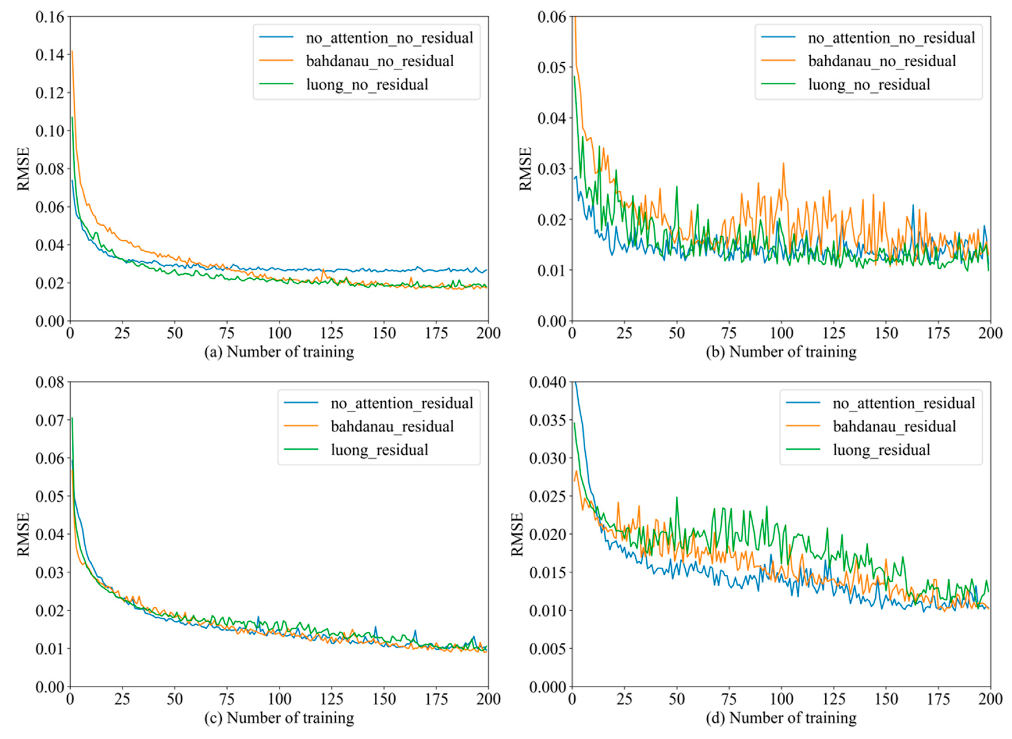
By selecting the coalescence of the Residual mechanism and the two Attention mechanisms for simulation verification in Figure 11, the training error, test error and training time of the model are compared, and the results are shown in

Table 1. The algorithm performance comparison between the Residual mechanism and the different Attention mechanisms.

Residual	Attention	Train		Test
		MSE	RMSE	MSE	RMSE
False	False	0.000711	0.027	0.000124	0.011
	Bahdanau	0.000297	0.017	0.000169	0.013
	Luong	0.000317	0.018	0.000198	0.014
True	False	0.000091	0.0095	0.000106	0.01
	Bahdanau	0.000083	0.0091	0.000104	0.01
	Luong	0.000112	0.0105	0.000155	0.012

.

In Table 1, true and false represent whether the model uses corresponding Residual or Attention mechanisms, respectively, and Table 1 shows that when the model adopts the Residual mechanism, the training error and test error of the model are significantly reduced. It is shown that the addition of the Residual mechanism improves the predictive performance of the model, compared with two different Attention mechanisms, the model adopts the Residual mechanism and the Bahdanau mechanism adopts the model with better performance, and the training error and test error value are minimal. Therefore, the Seq2seq model used for short-term load prediction adopts the combination of Residual mechanism and Bahdanau mechanism, as shown in Figure 12.

When the Seq2seq model is trained, an iterative prediction is used, and the accuracy of the experimental results is obtained by adjusting and selecting the parameters of the model in order to achieve the desired results. The model parameters are set as shown in

Table 2. Setting of model parameters.

Parameter	Parameter Setting	Parameter	Parameter Setting
Training data	7008	Test data	1752
Length input	24	Length output	1
Learning rate	0.01	Decay rate of learning rate	0.5
Node in hidden layer	100	Decay steps	200
Number of trainings	300	Batch	200
Optimization algorithm	Adam	Gradient value	5.0

.

Based on the large power system dataset, 80% of the data are used for training the model and remaining are used for testing of the model. The input length of the data is set to 24, and the output length of the data is set to 1, with a learning rate of 0.01 and a decay rate of 0.5. The hidden neurons of the Residual LSTM are set as 100, with 200 decay steps. The model is trained for up to 300 iterations with a batch size of 200. The Adam optimizer is used to minimize the loss function and the disturbance optimization. The gradient value is set to 5.0.

5.4. Experimental Results and Analysis

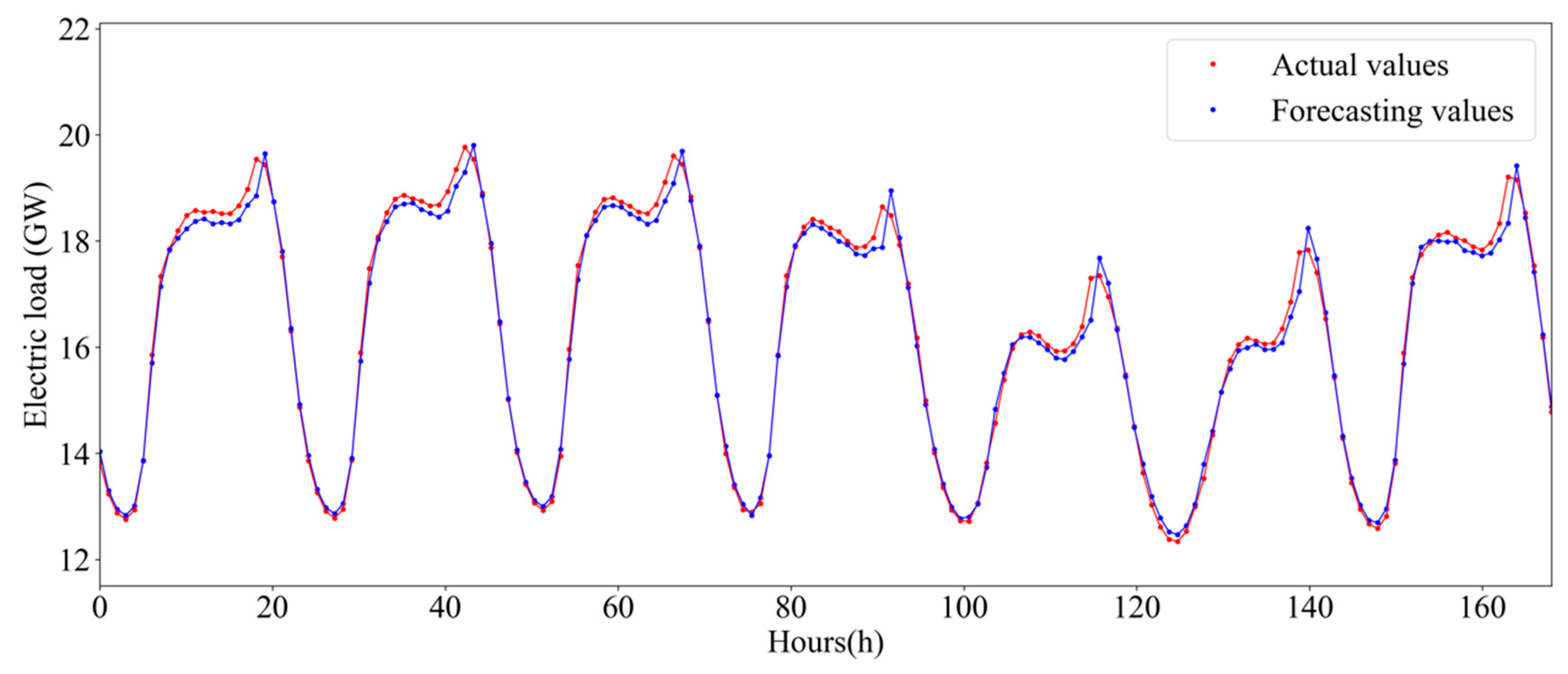
After the model training, the test data set is predicted. The test set data is used as input to the model once it has been trained, and the input data is computed by the model to obtain the predicted values, and the forecast results obtained by the load prediction model are compared with the real values. It can be seen in Figure 13 that the predicted value and the true value basically coincide with each other.

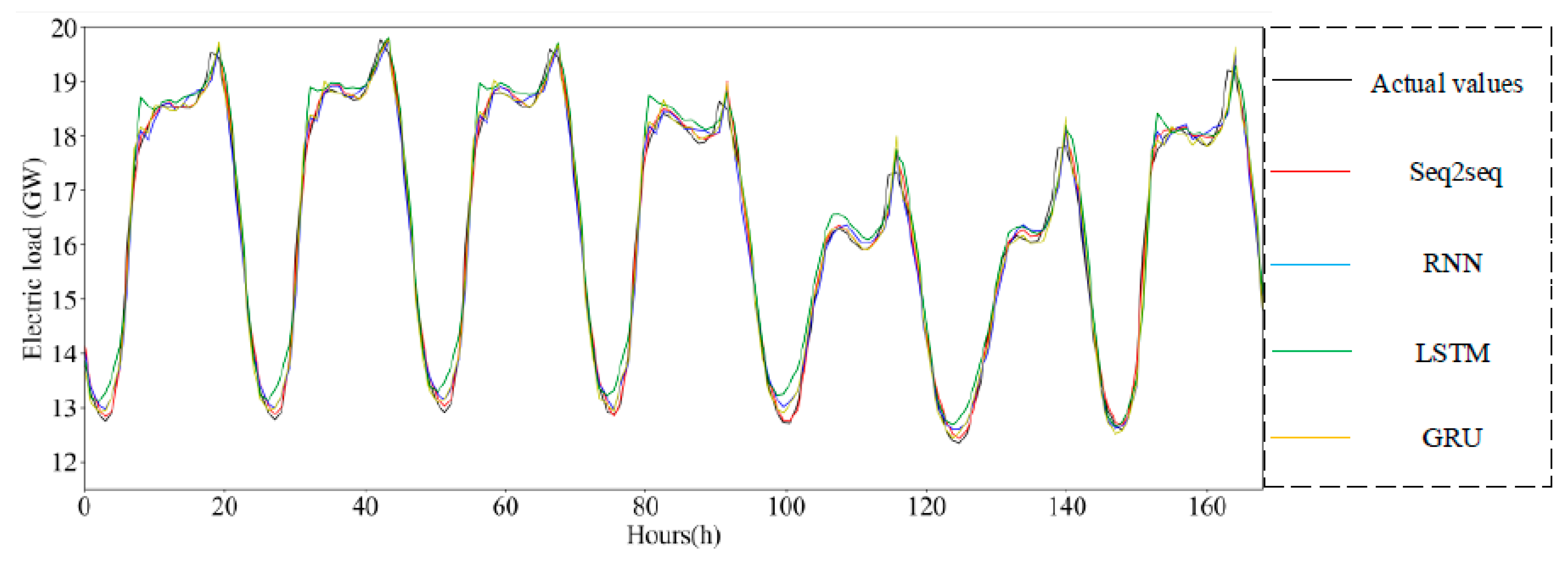
In this paper, the performance shows that the load prediction model with Seq2seq has stronger optimization capabilities. To demonstrate the superiority of the proposed method, compared with the optimal results, the initial and optimal fitness of the Seq2seq model was significantly superior to the results of the RNN, LSTM, and GRU models. The comparison graph is shown in Figure 14.

In Figure 14, it can be observed that, compared to RNN, LSTM, and GRU, the short-term load forecasting using Seq2seq model is better. The prediction results obtained by the Seq2seq model proposed in this paper are smooth, and the fitting effect is good. The error between the prediction result and the real value obtained by the RNN, LSTM, and GRU algorithms is large. The errors under different algorithms are shown in

Table 3. The comparison of prediction errors of normalized data under different algorithms.

Different Method	Error of Normalized Data
	MSE	RMSE	MAE	MAPE
Seq2seq	0.000083	0.0091	0.0076	5.20%
RNN	0.00019	0.0138	0.01015	7.35%
LSTM	0.00039	0.01964	0.0158	14.04%
GRU	0.0002	0.01449	0.01066	8.29%

and

Table 4. The comparison of the prediction errors of the raw data under different algorithms.

Different Method	Error of Raw Data
	MSE	RMSE	MAE	MAPE
Seq2seq	0.0319	0.1787	0.1347	0.8262%
RNN	0.0599	0.2448	0.1799	1.1143%
LSTM	0.1212	0.3482	0.2809	1.7847%
GRU	0.0659	0.2567	0.1890	1.1760%

.

It can be observed from the above table that short-term load prediction is used by the algorithm of this paper, and the errors are comparatively smaller than for the RNN, LSTM and GRU algorithms, showing that it has a better prediction effect.

5.5. Supplementary Experiment

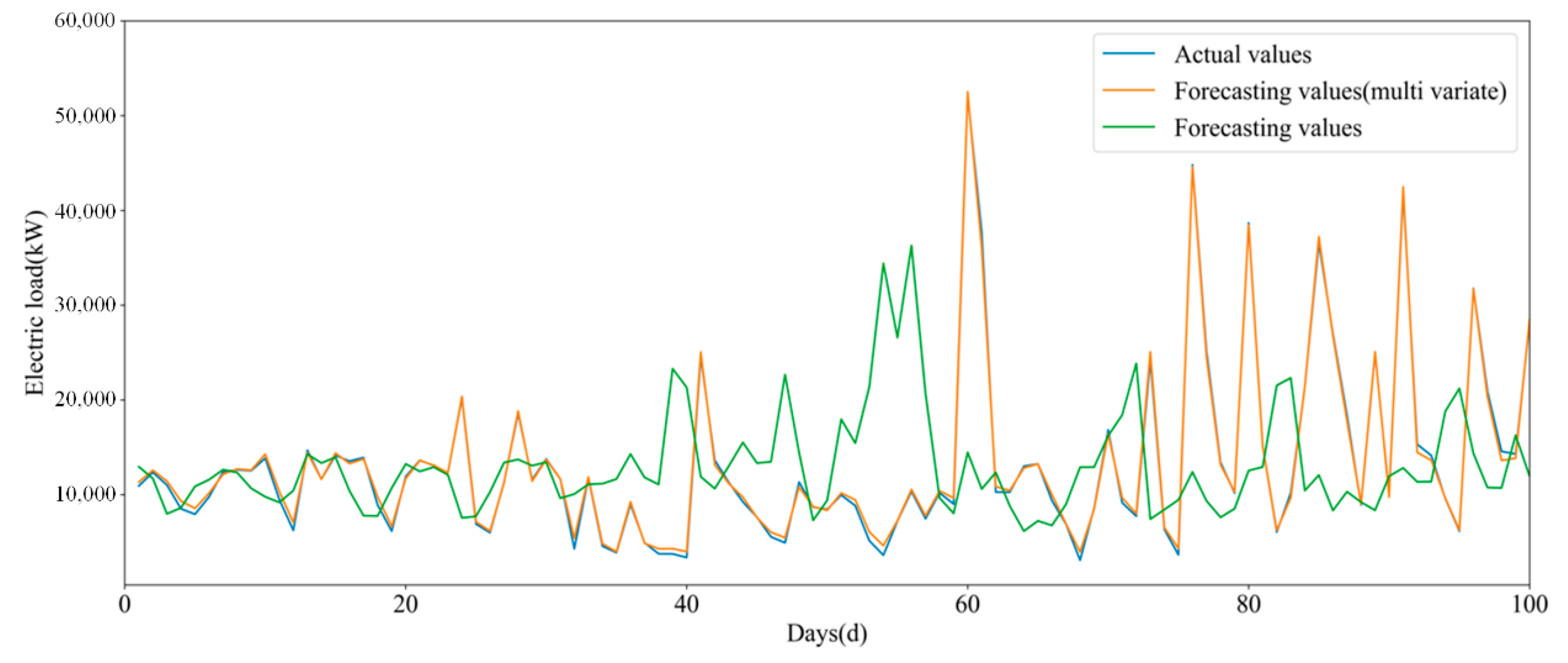
To illustrate that this experiment shows better prediction results for the load forecasting of small power grids, this paper uses the data of a small power grid as the experimental data set, and uses the Seq2seq proposed in this paper to carry out load forecasting. In [38], the authors considered the impact of different types of day, which is important for load prediction. In the forecasting process, the weather (temperature, holidays, and humidity, etc.) data were also used as input variables. The detailed input data types are shown in

Table 5. The specific meaning of input data.

Type of Data	Specific Meaning
F_day1	Load value one day before the date to be tested
F_week	The load value of the day of the previous week
Day of week	Which day of the week
Workday	Whether it is working day or not
Holiday	Whether it is a holiday or not
Tem_max	Maximum temperature
Tem_min	Minimum temperature
RH_max	Maximum humidity
RH_min	Minimum humidity

. In addition, the experimental results with a comparatively minimized error were obtained, as shown in Figure 15 and Figure 16.

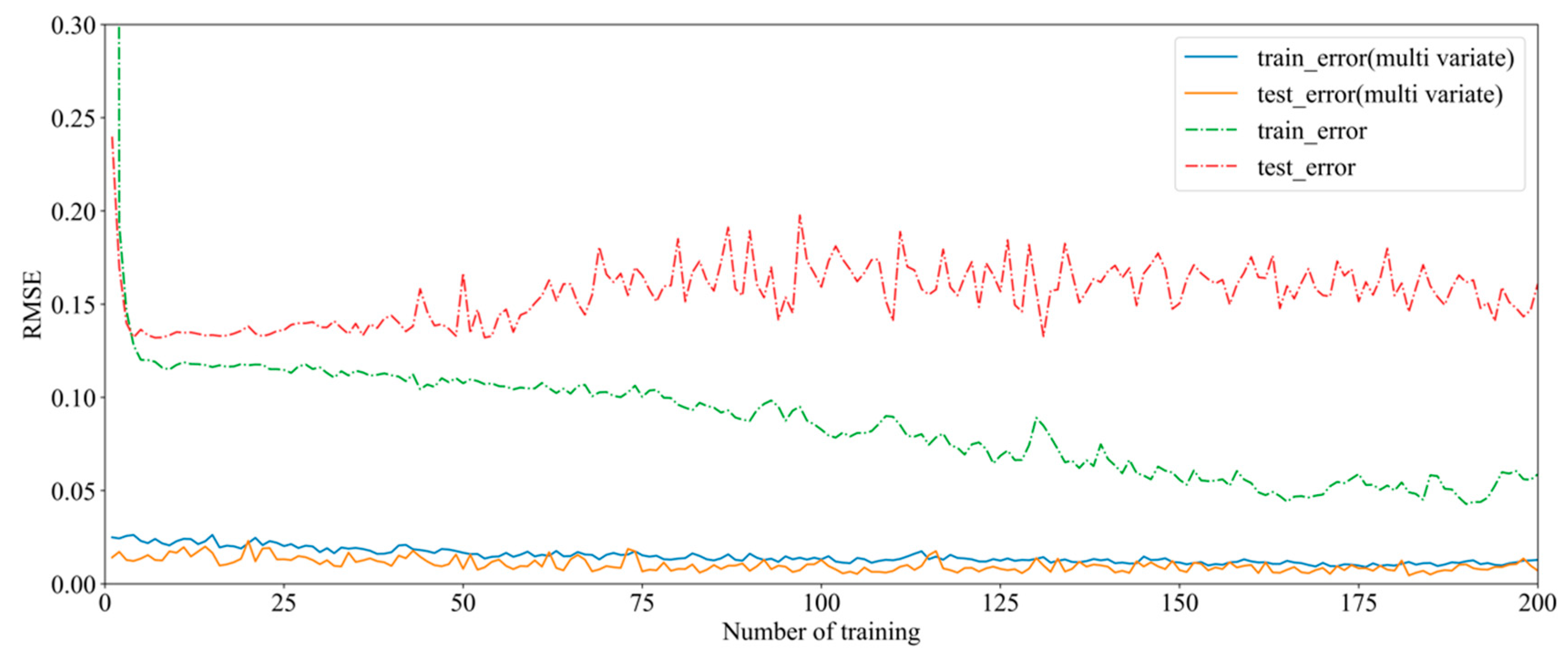
It can be observed from Figure 15 and Figure 16, that for load forecasting, if more parameters such as date and weather are selected under the same model training parameters, it will improve the model learning. With the same training times, if other relevant features are introduced, the learning performance of the model will be much higher than that of the pure load data training, and the accuracy of the model is improved when the training data is small, also improving the overall model prediction accuracy. In terms of training the model with large and small power system data, the proposed model exhibits smooth behavior, as seen in Figure 15, and thus the model can be considered to be more stable.

6. Conclusions

The outcomes of load forecasting are conducive to determining the power that needs to be generated in the coming days, the installation of new generator sets in the future, the determination of the size, location and time of the installed capacity, the determination of capacity expansion and reconstruction of the power grid, and the determination of the construction and development of the power grid. Moreover, it assists in the stable operation of the power system by predicting the demand. Therefore, the accuracy of load forecasting directly affects the stable and efficient operation of the power grid. This paper proposes a novel Seq2seq model for more precise power system load forecasting.

The main contributions of this paper are as follows:

(1)

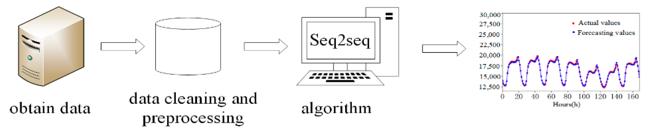
The progressive application of the Seq2seq model for load forecasting. Initially, the model was widely used in the field of machine translation, and it has been used for load forecasting to obtain better load forecasting results.

(2)

According to the periodic characteristics of historical load data, the correlation coefficient method is used to determine the order of the input historical load, and the accuracy of data feature extraction is improved.

(3)

The coalescence of Residual and Attention mechanisms is used to optimize the Seq2seq model, which overcomes shortcomings, such as model instability and lower precision, ensuring the effectiveness of power load forecasting.

(4)

To demonstrate the robustness and the stability of the proposed model, the electricity dataset of the small power grid is used for prediction, also considering different weather conditions and user behaviors.

In this paper, the short-term load prediction model based on LSTM’s Seq2seq algorithm is developed by the coalescence of the Residual and Attention mechanism, and the effective characteristics of historical load data are extracted using the model. This reduces the error of short-term load prediction, eventually improving the prediction performance of the model and presenting a new method for short-term load prediction. By constantly optimizing the performance of various deep learning algorithm to improve the prediction accuracy, it will be possible to further develop a more advanced, faster and more accurate model for load prediction.

In the future, we look forward to studying the method’s applicability for long-term forecasting. Moreover, price prediction with respect to load forecasting can be studied comparatively. Furthermore, efficiency and prediction accuracy of load forecasting may be improved by combining various forecasting methods in order to develop a robust and stable forecasting model.