Research on Large-Signal Stability of DC Microgrid Based on Droop Control

Abstract

Ensuring the large signal stability of the DC microgrid is the premise of the safe operation of the DC microgrid, but the research on the large-signal stability of microgrids with multiple droop control micro-sources is still scarce. In this paper, a DC microgrid system model with multiple droop control micro-sources was established by appropriate simplification. Addressing the problem that most stability research methods cannot be quantitatively analyzed, the mixed potential function method was used to analyze the large signal stability of the system. However, the criterion obtained by the conventional mixed potential function method is complicated and contains multiple time-varying parameters, which is not convenient for analysis. Therefore, the simple form of the criterion was obtained through simplification and the analysis proved the rationality of the simplification. On this basis, a nonlinear droop control method was proposed to improve the anti-interference ability of the system. Finally, the accuracy of the large signal stability criterion and the effectiveness of nonlinear droop control on the system’s large signal stability were verified by simulation.

1. Introduction

As a way to ensure reliable and efficient access to distributed power grids, the DC microgrid has more advantages than the AC microgrid as (1) it requires less converters, which is more concise and efficient; and (2) there is no frequency problem, therefore, its control system is simpler and more reliable [1,2]. At present, DC microgrids are widely used in aviation, submarine, and other fields, and has received increasing attention [3]. In the DC microgrid, each micro-source, energy storage device, and load device is connected in parallel to the DC bus through the converters, therefore, ensuring the stability of the DC bus voltage is a key issue for the stable operation of the DC microgrid [4].

The stability analysis of microgrid systems can be divided into small signal stability analysis and large signal stability analysis. At present, the research on DC microgrid stability analysis focuses on small signal stability [5,6]. Small signal stability can ensure the stability of the system at the equilibrium point, but the boundary of the stability domain cannot be determined, and there are limitations when the system has large disturbances. Analysis of large signal stability is even more essential, especially in DC microgrids with frequent load and micro-source switching.

As the DC microgrid system has the characteristics of nonlinearity and strong coupling, the analysis method based on linearization theory is not applicable. Lyapunov’s second method is widely used in the stability analysis of a nonlinear system [7]. Based on Lyapunov’s second method and in consideration of different perspectives, researchers have proposed some stability analysis methods. From the perspective of illustration, [8,9] used the phase plane method to analyze the large signal stability of the cascaded DC system, and judged the stability of the system when the system’s parameters changed through the trajectory map. However, this method failed to obtain the stability criterion of the analytical form and is difficult to analyze in a high-order system. From the perspective of linear fitting, [10,11] used the T-S multi-model method to establish the Lyapunov function of the DC power supply system, and quantitatively analyzed the large signal stability of the system. However, this method is difficult to implement in a closed-loop controlled system. From the point of energy, [12,13] obtained the stability criterion under a large disturbance of the DC microgrid with a damped filter and a constant power load (CPL) by means of the mixed potential function method. Although the stability criterion obtained by this method is somewhat conservative, it is simple and easy toanalyze.

However, all of the above studies have only proposed stability criteria for cascaded systems or single-supply systems, and have not addressed cases where multiple closed-loop controlled micro-sources are co-powered. In fact, for DC microgrids with multiple droop controlled micro-sources, the existence of multiple control loops makes quantitative analysis more difficult [14,15].

In [16], based on the analysis and simulation study, the criterion of the large signal stability of the droop controlled microgrid was proposed and modified based on the mixed potential function method, however, the criterion requires the power distribution information at a steady state and is too complicated when multiple micro-sources are connected in parallel, which is not conducive to stability analysis.

Aimed at the above problems, this paper established a DC microgrid system model with multiple droop controlled micro-sources by appropriate simplification, used the mixed potential function method to quantitatively analyze the system stability, then obtained a simple form of the stability criterion through simplified calculation and the rationality of this step was also analyzed. On this basis, a nonlinear droop control method was proposed to improve the large signal stability of the system. Finally, the simulation verified the correctness of the obtained criterion and the validity of the nonlinear droop control strategy.

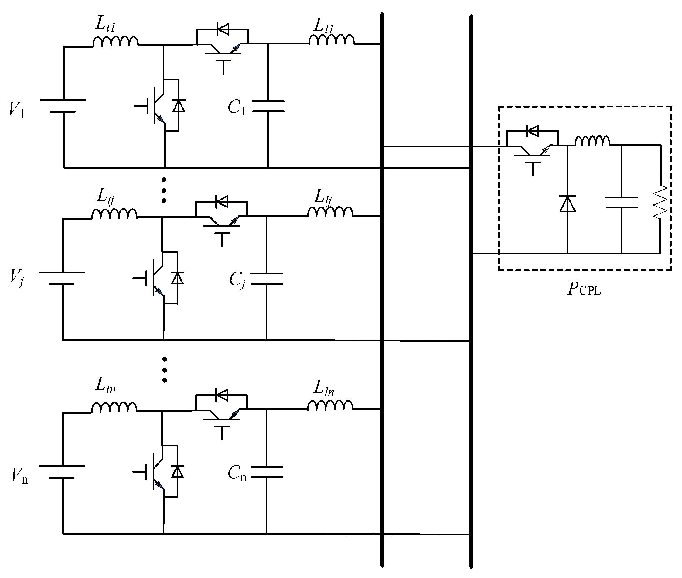
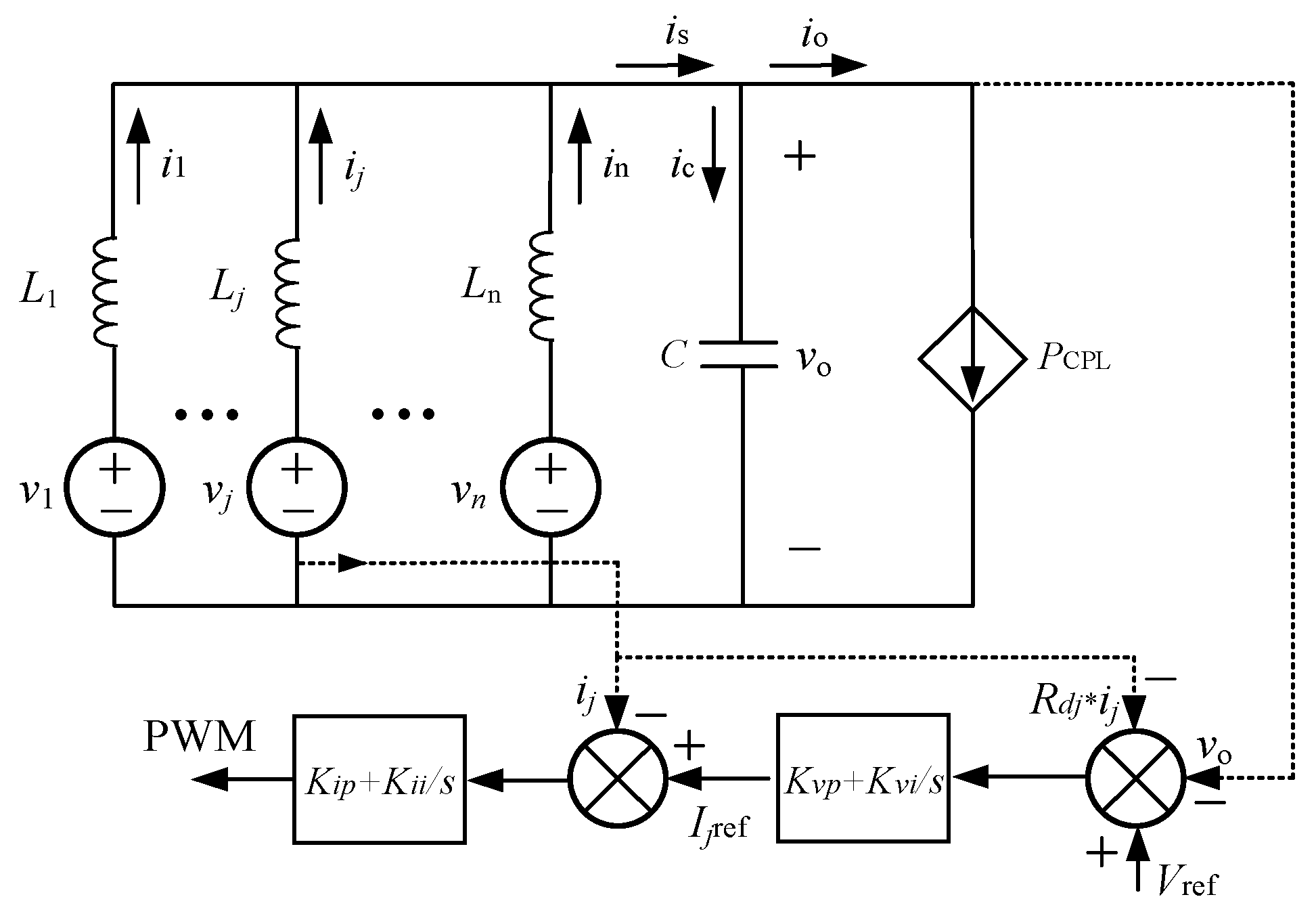
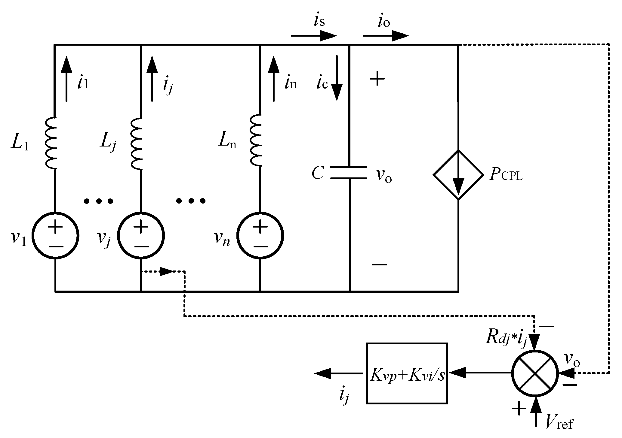
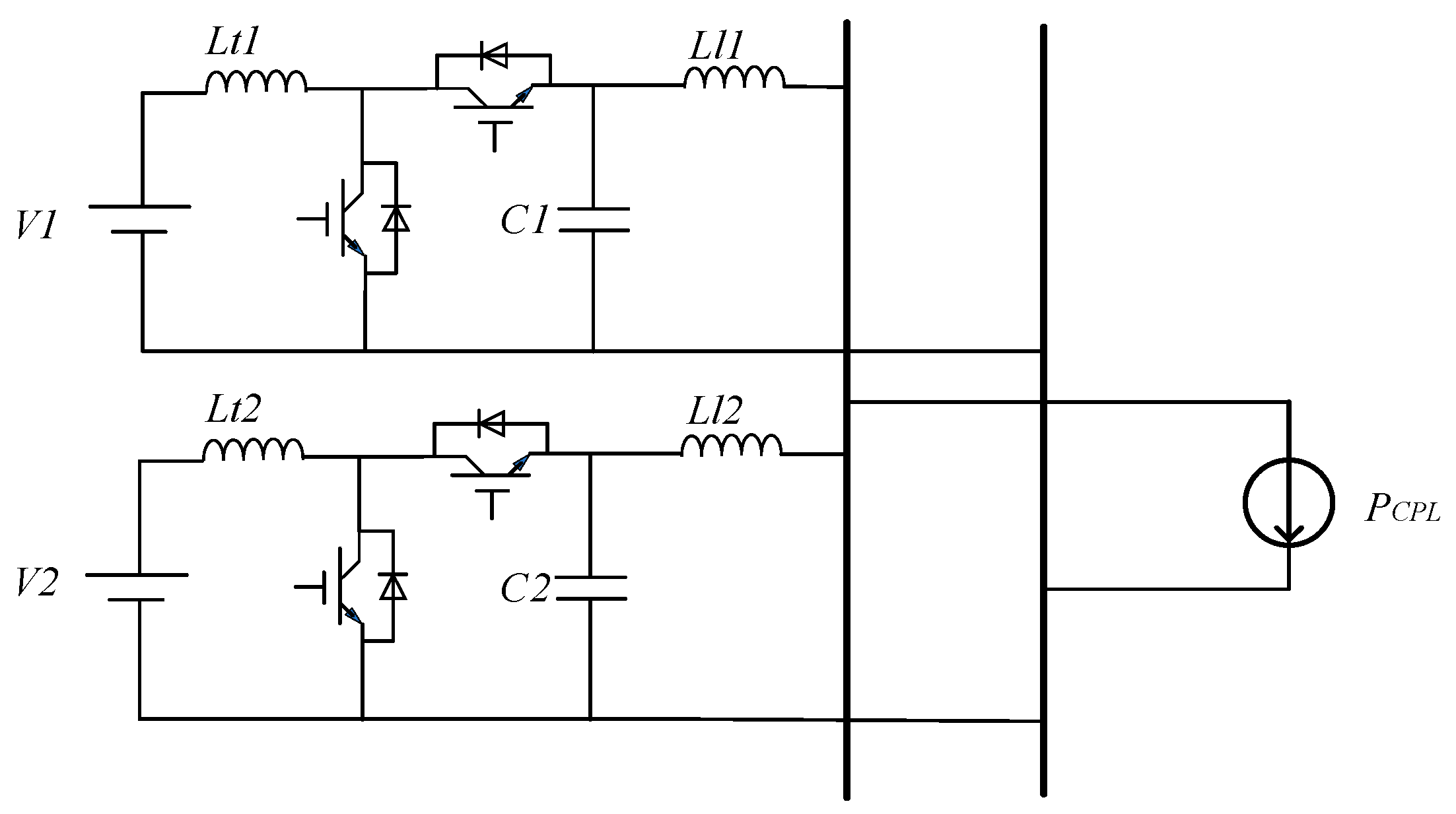
2. DC Microgrid Structure and Large Signal Model

In general, DC microgrids include distributed micro-sources, batteries, constant power loads, and a large number of power electronic converters. Among them, each battery is connected to the bus through the bidirectional DC/DC converter, and the droop control strategy is used to realize the power distribution without communication; the distributed micro-sources often work in the Maximum Power Point Tracking (MPPT) mode and can be regarded as a negative constant power load in a short time [17]. Therefore, the distributed micro-sources and constant power load can be uniformly equivalent to a constant power load. The typical structure of a DC microgrid was the system studied in this paper, and its structure is shown in Figure 1.

Among them, L_tj, C_j, L_lj (j = 1,2…n) are the inductance, capacitance, and line inductance of each micro-source converter and R_dj is the droop coefficient of the jth micro-source (j = 1,2…n). In the modeling process, the following assumptions and equivalents were made: (1) Considering that the droop coefficient can be equivalent to a series resistor in the DC microgrid, which is usually much larger than the line resistance, the line resistance can be ignored; and (2) Combining the output reactance and line reactance of each converter into the equivalent reactance L_j (j = 1,2…n), and concentrating the capacitance of each converter as a large capacitor C. The simplified equivalent circuit diagram of the DC microgrid system is shown in Figure 2.

In Figure 2, V_ref is the voltage reference value; v_o is the bus voltage; v_j and i_j are the output voltage and output current of the jth micro-source, respectively (j = 1,2…n); i_o, i_c are the load current and the capacitor current, respectively; i_s is the sum of the output currents of all micro-sources; and P_CPL is the power of the equivalent CPL. The mathematical model of the system is as follows:

$$\{\begin{array}{l}{L}_j\frac{d{i}_j}{dt}=v_j-v_{\mathrm{o}}\\ C\frac{d{v}_o}{dt}=i_s-i_o\\ i_s=i_1+i_2+...+i_n\\ i_o=\frac{P_{CPL}}{v_o}\end{array}$$

(1)

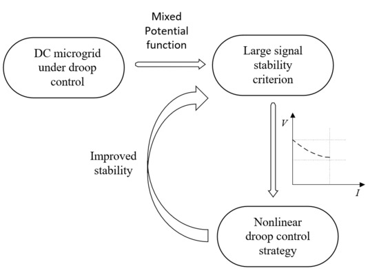
3. Application of Mixed Potential Function Method in the DC Microgrid

3.1. Mixed Potential Function Theory

The theory of mixed potential functions was proposed by R.K. Brayton and J.K. Moser in 1964 and is mainly used to study the stability of nonlinear circuits [18,19]. The mixed potential function theory holds that for different structures of RLC nonlinear circuit networks, the difference equation can be expressed as follows:

$$\{\begin{array}{l}L\frac{d{i}_{\rho }}{dt}=\frac{\partial P(i,v)}{\partial i_{\rho }}\\ C\frac{d{v}_{\sigma }}{dt}=\frac{\partial P(i,v)}{\partial v_{\sigma }}\end{array}$$

(2)

where i_ρ represents the inductor current and v_σ represents the capacitor voltage. P(i,v) is similar to the Lyapunov energy function, which contains a voltage potential function and a current potential function. The mixed potential function P is related to the distribution structure of the inductor, capacitor, and non-energy storage element in the circuit. The steps of constructing the mixed potential function are as follows:

• Calculate the potential function of all non-energy storage components in the circuit;
• Calculate the energy contained in the capacitive component of the circuit, that is, the product of the capacitor voltage and the capacitor current;
• Add the above two to obtain the mixed potential function of the circuit.

The unified expression of the mixed potential function is:

$$P(i,v)=-A(i)+B(v)+(i,\gamma v-\alpha )$$

(3)

where A(i) represents the current potential function of the non-energy storage element in the circuit; B(v) represents the voltage potential function of the non-energy storage element in the circuit; γ represents the constant matrix associated with the structure; and α is a constant vector. After constructing a mixed potential function, Equation (2) can be used to verify the correctness of the function.

The mixed potential function has three stability theorems, and the third one provides a theoretical basis for solving the stability boundary of the system under large signal disturbances. The specific derivation process will not be repeated here. Now, this stability theorem can be rewritten as follows:

Theorem 1.

Based on the uniform expression of the mixed potential function, define the following variables:

$$\{\begin{array}{c}{P}_i=\frac{\partial P(i,v)}{\partial i},P_v=\frac{\partial P(i,v)}{\partial v}\\ A_{ii}(i)=\frac{{\partial }^{2}A(i)}{\partial i^2},B_{vv}(v)=\frac{{\partial }^{2}B(v)}{\partial v^2}\end{array}$$

(4)

If μ₁ represents the minimum eigenvalue of the matrix L^−1/2A_ii(i) L^−1/2, μ₂ represents the minimum eigenvalue of the matrix C^−1/2B_vv(v) C^−1/2, where L and C are inductance matrix and capacitor matrix, respectively. If all currents i and voltages v in the circuit meet the conditions:

$${\mu }_1+{\mu }_2>0$$

(5)

When |v|+|i|→∞, and if expression (6) is satisfied:

$$P^{\ast }(i,v)=\frac{{\mu }_1-{\mu }_2}{2}P(i,v)+\frac{1}{2}{P}_i^T(L^{-1}{P}_i)+\frac{1}{2}{P}_v^T(C^{-1}{P}_v)\to \infty$$

(6)

Then, when the system response time t → ∞, the whole system will tend to be stable, and all solutions of the circuit will tend to the steady state value, which guarantees the large signal stability of the system.

3.2. Large Signal Stability Criterion of the System

The equivalent circuit of the DC microgrid system is shown in Figure 2. Assuming that the response speed of the inner current loop is fast enough that i_j can follow the current reference value i_ref output by the outer loop controller quickly, then the inner current loop can be ignored. The simplified equivalent circuit is shown in Figure 3.

According to Figure 3, the output current expression of each micro-source can be obtained as:

$$i_j=K_{vp}(V_j-v_o-R_{dj}\times i_j)+K_{vi}{\displaystyle {\int }_0^t(V_j-v_o-R_{dj}\times i_j)dt}$$

(7)

In Figure 3, the non-energy storage component in the DC microgrid system contains controlled current sources, and the constant power load, so the current potential function of the non-energy storage component is:

$${\displaystyle \int {\displaystyle \sum _{\mu }{v}_{\mu }}}d{i}_{\mu }={\displaystyle \sum _{j=1}^n{\displaystyle {\int }_0^{i_j}{v}_{o}di}-}{\displaystyle {\int }_0^{i_o}\frac{P_{CPL}}{i_o}di}={\displaystyle \sum _{j=1}^n{v}_o{i}_j}-{\displaystyle \sum _{j=1}^n{\displaystyle {\int }_0^{v_o}{i}_{j}dv}}-P_{CPL}+{\displaystyle {\int }_0^{v_o}\frac{P_{CPL}}{v_o}dv}$$

(8)

The energy of the capacitor branch is:

$${\displaystyle \sum _{\sigma }{v}_{\sigma }{i}_{\sigma }}=-v_o(i_s-\frac{P_{CPL}}{v_o})=-{\displaystyle \sum _{j=1}^n{v}_o{i}_j}+P_{CPL}$$

(9)

So, the mixed potential function is:

$$P(i,v)={\displaystyle \int {\displaystyle \sum _{\mu }{v}_{\mu }}}d{i}_{\mu }+{\displaystyle \sum _{\sigma }{v}_{\sigma }{i}_{\sigma }}={\displaystyle {\int }_0^{v_o}\frac{P_{CPL}}{v_o}dv}-{\displaystyle \sum _{j=1}^n{\displaystyle {\int }_0^{v_o}{i}_{j}dv}}$$

(10)

As shown in Equation (11), the constructed mixed potential function P(i,v) is reasonable because it satisfies Equation (2).

$$\frac{\partial P(i,v)}{\partial v_o}=\frac{P_{CPL}}{v_o}-{\displaystyle \sum _{j=1}^n{i}_j}=-C\frac{d{v}_{dc}}{dt}$$

(11)

Write the uniformed expression of the mixed potential function as shown in Equation (12):

$$\{\begin{array}{c}A(i)=0\\ B(v)={\displaystyle {\int }_0^{v_o}\frac{P_{CPL}}{v_o}dv}-{\displaystyle \sum _{j=1}^n{\displaystyle {\int }_0^{v_o}{i}_{j}dv}}\\ (i,\gamma v-\alpha )=0\end{array}$$

(12)

Then, there is:

$$A_{ii}(i)=\frac{{\partial }^{2}A(i)}{\partial i^2}=0$$

(13)

$$\frac{\partial B(v)}{\partial v_o}=\frac{P_{CPL}}{v_o}-{\displaystyle \sum _{j=1}^n{i}_j}$$

(14)

$$\frac{{\partial }^{2}B(v)}{\partial v_o^2}=-\frac{P_{CPL}}{v_o^2}-{\displaystyle \sum _{j=1}^n\frac{\partial i_j}{\partial v_o}}$$

(15)

For Equation (7), the ∫(V_j-v_o-R_dj∙i)dt term can be ignored (see Appendix A for the plausibility of this step), and taking the derivative of v_o at both ends of the equation, Equation (16) can be obtained:

$$\frac{\partial i_j}{\partial v_o}=K_{vp}(-1-R_{dj}\frac{\partial i_j}{\partial v_o})$$

(16)

Then,

$$\frac{\partial i_j}{\partial v_o}=\frac{-K_{vp}}{1+K_{vp}{R}_{dj}}$$

(17)

Bring Equation (17) into Equation (15) to obtain

$$\frac{{\partial }^{2}B(v)}{\partial v_o^2}=-\frac{P_{CPL}}{v_o^2}+{\displaystyle \sum _{j=1}^n\frac{K_{vp}}{1+K_{vp}{R}_{dj}}}$$

(18)

Therefore, the minimum eigenvalue μ₁ of the matrix L^−1/2A_ii(i) L^−1/2 and the minimum eigenvalue μ₂ of the matrix C^−1/2B_vv(v) C^−1/2 is

$$\{\begin{array}{c}{\mu }_1=0\\ {\mu }_2=-\frac{P_{CPL}}{C{v}_o^2}+\frac{1}{C}{\displaystyle \sum _{j=1}^n\frac{K_{vp}}{1+K_{vp}{R}_{dj}}}\end{array}$$

(19)

According to the third stability theorem of the mixed potential function theory, the large signal stability criterion of the DC microgrid is:

$$-\frac{P_{CPL}}{v_o^2}+{\displaystyle \sum _{j=1}^n\frac{K_{vp}}{1+K_{vp}{R}_{dj}}>0}$$

(20)

That is:

$$P_{CPL}<{\displaystyle \sum _{j=1}^n\frac{K_{vp}{v}_o^2}{1+K_{vp}{R}_{dj}}}$$

(21)

From criterion (21), as the droop coefficient R_dj decreased, the maximum allowable value of P_CPL increased, indicating that the system’s large signal stability margin was improved. On this basis, a nonlinear droop control method was proposed to improve the stability margin of the DC microgrid system.

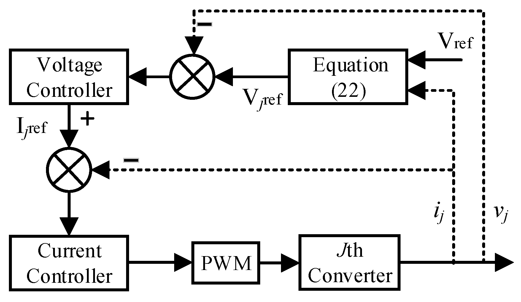
4. Nonlinear Droop Control Strategy

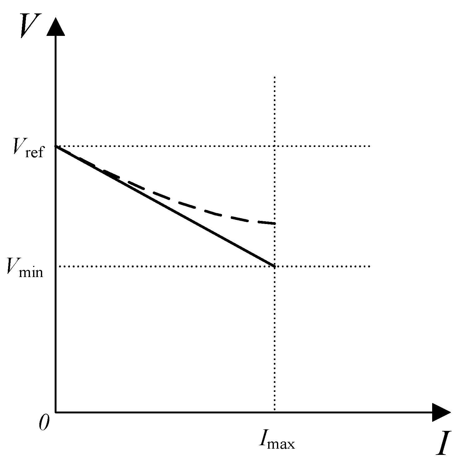
4.1. Design of Nonlinear Droop Curve

The traditional droop control uses a linear droop curve, and the droop coefficient does not change. Therefore, the bus voltage drop is large and the stability margin may be insufficient under a heavy load. To address this problem, this paper improved the large signal stability of the system and reduced the bus voltage drop by adaptively changing the droop coefficient. Selecting the adaptive droop coefficient means designing a nonlinear droop curve in the U–I diagram of the converter output. From a practical point of view, the droop curve should meet the following requirements:

• The starting point of the droop curve should be set at the initial voltage point of the unloaded state.
• The abscissa of the end point of the droop curve is the maximum current value allowed to flow through the inverter, and the ordinate is the lowest allowable voltage value of the bus.
• The droop curve should be designed between the start and end points. As the system may oscillate when running near the non-lead point on the droop curve [20,21], the droop curve needs to be smooth, that is, continuous.

As shown in Figure 4, the solid line is a conventional droop curve, and the dashed line is the proposed nonlinear droop curve, where the slope gradually decreases as the current increases. Combined with the previous analysis, it can be seen that the nonlinear droop curve can improve the maximum allowable value of P_CPL by reducing the slope of the droop curve, especially in the case of a heavy load, which can greatly improve the stability margin of the system. Furthermore, when the load of the system is greatly disturbed, the gentle droop curve can effectively limit the drop in DC bus voltage that maintains the bus voltage stability, thus ensuring the stable operation of the system.

The implementation of the target curve is to add a quadratic term of current with a positive coefficient to the traditional drooping curve equation, so that the linear droop curve can be changed to a nonlinear curve with a decreasing slope. The initial value of the voltage is determined, and since the slope is decreasing, the voltage drop of the curve on the same abscissa is smaller than that of the linear droop curve and does not exceed the maximum allowable value.

The expression of the nonlinear curve is as shown in Equation (22), and is obviously steerable everywhere, thus the three requirements of the curve design can be satisfied.

$$v_o=v_{ref}+a{i}^2-bi$$

(22)

where v_ref is the voltage reference value; v_o, i are the output voltage and current of the inverter, respectively; and a, b are the droop coefficients.

As for the configuration of the drooping parameters, a, b, it is necessary to ensure that the output of each micro-source is distributed according to the rated power at the steady state, and ideally are:

$$\frac{i_i}{i_j}=\frac{P_i}{P_j}$$

(23)

By Equation (22):

$$v_{ref}-v_o=b_i{i}_i-a_i{i}_i{}^2=b_j{i}_j-a_j{i}_j{}^2$$

(24)

where a_i, b_i, i_i, P_i and a_j, b_j, i_j, P_j are the droop coefficients, output current, and rated power of converter i and converter j, respectively.

Obviously, the power distribution of different micro-sources satisfies Equation (23) at the steady state when their droop coefficients are configured according to Equation (25), that is, according to the rated power.

$$\{\begin{array}{c}\frac{a_i}{a_j}=\frac{P_j^2}{P_i^2}\\ \frac{b_i}{b_j}=\frac{P_j}{P_i}\end{array}$$

(25)

The control block diagram of the proposed strategy is shown in Figure 5. As shown, the droop equation provides the reference value for the output voltage of the jth converter and serves as the input for the dual-loop control.

4.2. Large Signal Stability Analysis with Nonlinear Droop Control

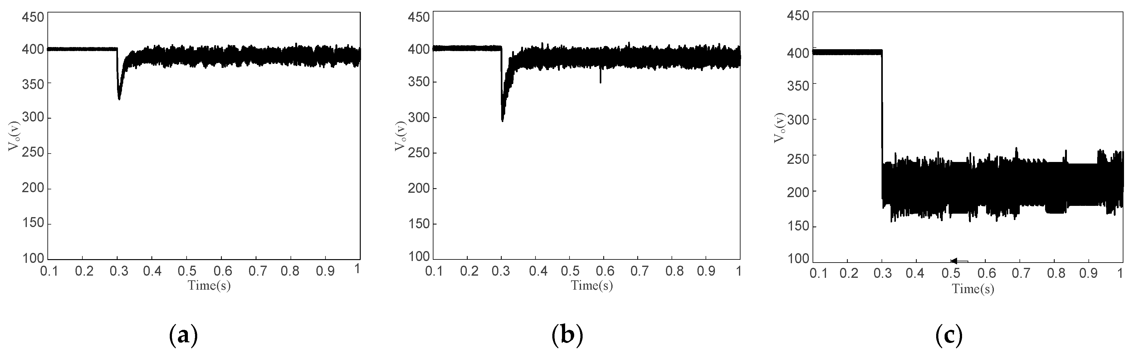
According to Equations (7) and (22), the output current expression of each micro-source can be expressed as shown in Equation (26):

$$i_j=K_{vp}(V_j-v_o-b_j{i}_j+a_j{i}_j^2)$$

(26)

Then,

$$\frac{\partial i_j}{\partial v_o}=\frac{-K_{vp}}{1+K_{vp}(b_j-2a_{j}i)}$$

(27)

Similar to the analysis in Section 3.2,

$$A_{ii}(i)=\frac{{\partial }^{2}A(i)}{\partial i^2}=0,$$

(28)

$$\frac{{\partial }^{2}B(v)}{\partial v_o^2}=-\frac{P_{CPL}}{v_o^2}+{\displaystyle \sum _{j=1}^n\frac{K_{vp}}{1+K_{vp}(b_j-2a_{j}i)}}$$

(29)

Then, the minimum eigenvalue μ₁ of the matrix L^−1/2A_ii(i) L^−1/2 and the minimum eigenvalue μ₂ of the matrix C^−1/2B_vv(v) C^−1/2 are:

$$\{\begin{array}{c}{\mu }_1=0\\ {\mu }_2=-\frac{P_{CPL}}{C{v}_o^2}+\frac{1}{C}{\displaystyle \sum _{j=1}^n\frac{K_{vp}}{1+K_{vp}(b_j-2a_{j}i)}}\end{array}$$

(30)

Therefore, the system’s large signal stability criterion is

$$-\frac{P_{CPL}}{v_o^2}+{\displaystyle \sum _{j=1}^n\frac{K_{vp}}{1+K_{vp}(b_j-2a_{j}i)}>0}$$

(31)

That is,

$$P_{CPL}<{\displaystyle \sum _{j=1}^n\frac{K_{vp}{v}_o^2}{1+K_{vp}(b_j-2a_{j}i)}}$$

(32)

Compared with criterion (21), if coefficient b is equal to the linear droop coefficient R_dj, the maximum allowable value of P_CPL in Equation (32) is larger, that is, the system’s large signal stability is improved.

5. Simulation

In order to verify the accuracy of the large signal stability criterion (21) and the effectiveness of the nonlinear droop control strategy, a DC microgrid with two micro-sources under droop control was constructed with MATLAB (R2016b)/Simulink, which is shown in Figure 6. The bus voltage was 400 V, the micro-source output voltage was 200 V, and the ratio of the rated power was 3:4 (P₁:P₂).The initial value of P_CPL was 23,000 W. The parameters of the system are shown in

Table 1. Parameters of the simulation model.

Parameters	Value
Inductance of converter1 (Lt1)	0.1 mH
Inductance of converter2 (Lt2)	0.15 mH
Capacitance of converter1 (C1)	1000 μF
Capacitance of converter2 (C2)	2000 μF
Line inductance of micro-source1 (Ll1)	70 μH
Line inductance of micro-source1 (Ll2)	40 μH
Droop coefficient of micro-source1 (Rd1)	0.8
Droop coefficient of micro-source1 (Rd2)	0.6
Proportional coefficient of voltage loop (Kvp)	0.1
Integral coefficient of voltage loop (Kvi)	80
Proportional coefficient of current loop (Kip)	20
Integral coefficient of current loop (Kii)	100
Switching frequency	20 kHz
Output voltage of load	200 V

. In the simulation experiment, the large disturbance of the CPL was simulated by changing P_CPL at 0.3 s.

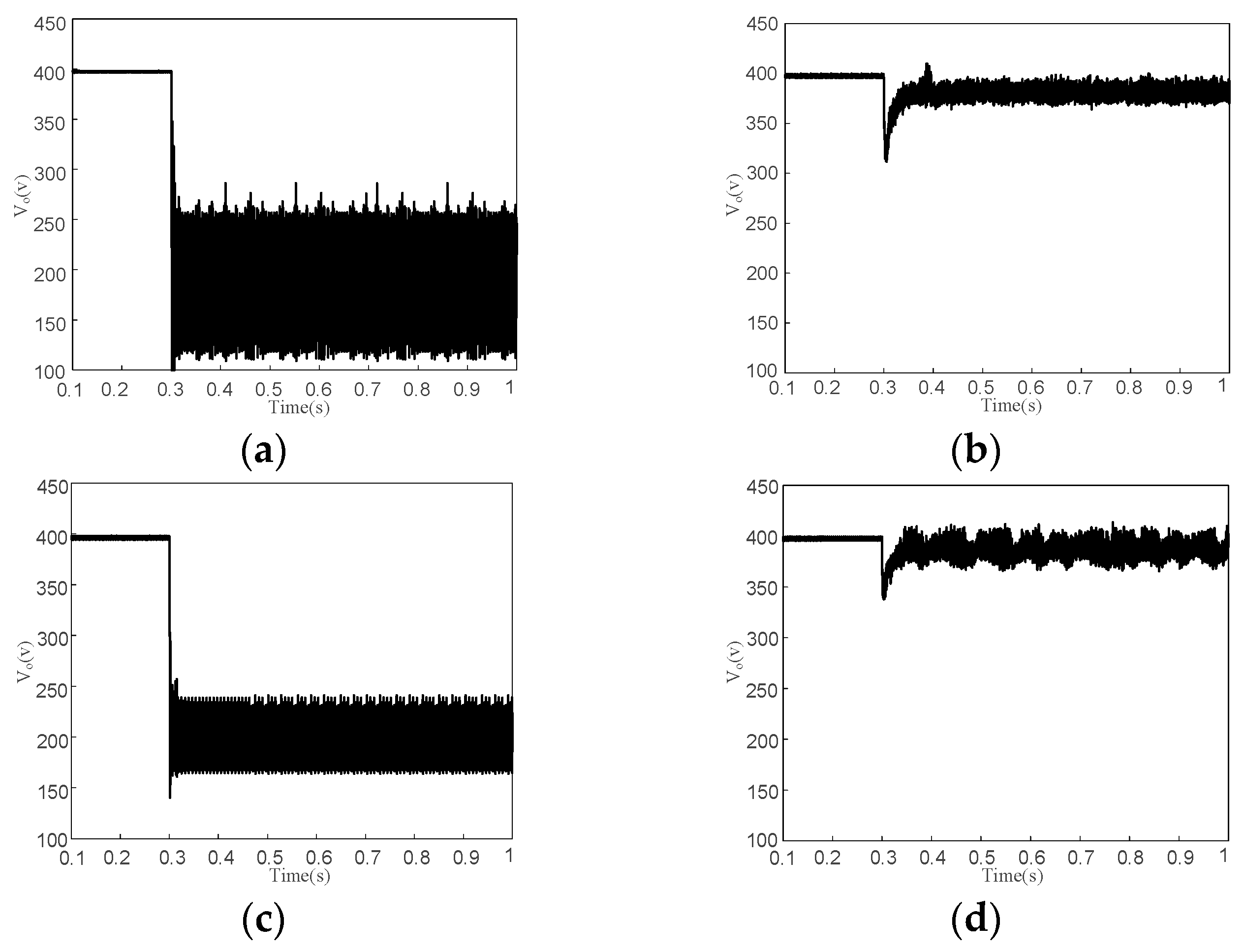
5.1. Verification of Large Signal Stability Criteria with Conventional Droop Control

According to the parameters provided in Table 1, and substituting them into Equation (21), the maximum allowable value of P_CPL was calculated to be 31,778 W. Figure 7a–c show the waveforms of the DC bus voltage when the power of constant power load was abruptly changed to 25,400 W, 34,300 W, and 36,100 W, respectively. The system remained stable when P_CPL was abruptly changed to 25,400 W, which is less than the maximum allowable value calculated by the criterion. As shown in Figure 7a, the system finally returned to the equilibrium point. In the case of Figure 7b, the constant power load after the mutation was slightly larger than the maximum allowable value, and the system was still stable. However, this does not mean that the large signal stability criterion is wrong as the large signal stability criterion obtained by the mixed potential function method is a sufficient condition, and not a necessary and sufficient condition, so when P_CPL is slightly larger than the maximum allowable value, it may still be a stable large signal. When the constant power load reached 36,100 W, the bus voltage failed to return to the equilibrium point and collapsed after the disturbance, therefore, the system lost stability. It can be seen that the maximum allowable value of P_CPL obtained by criterion (21) was similar to the simulation result (between 34,300 W and 36,100 W), which satisfied the stability criterion.

The influence of other parameters on system stability was also analyzed from another aspect. Taking the situation in Figure 7c, for example, where P_CPL was fixed at 36,100 W. As shown in

Table 2. Four sets of parameters and the calculations on stability.

Sequence Number	Kvp	Rd1	Rd2	Calculation Result
1	0.05	0.8	0.6	Unstable
2	0.15	0.8	0.6	Stable
3	0.15	2.8	2.1	Unstable
4	0.15	0.4	0.3	Stable

, four sets of parameters were selected and the system stability judged by calculation according to Equation (21).

Figure 8 shows the waveforms of the DC bus voltage under four sets of parameters ((a),(b),(c) and (d), which correspond to 1,2,3, and 4, respectively). In the No. 1 and No. 2 set of parameters, R_d1 and R_d2 remained unchanged while K_vp changed, which led to two different stability calculation results. In the No. 3 and No. 4 set of parameters, K_vp remained unchanged while R_d1 and R_d2 changed. We found that the system became stable with the decrease of droop coefficients R_d1 and R_d2, as seen in Figure 8. In conclusion, the calculation results were in accordance with the simulation results, thus verifying the validity of the stability criterion.

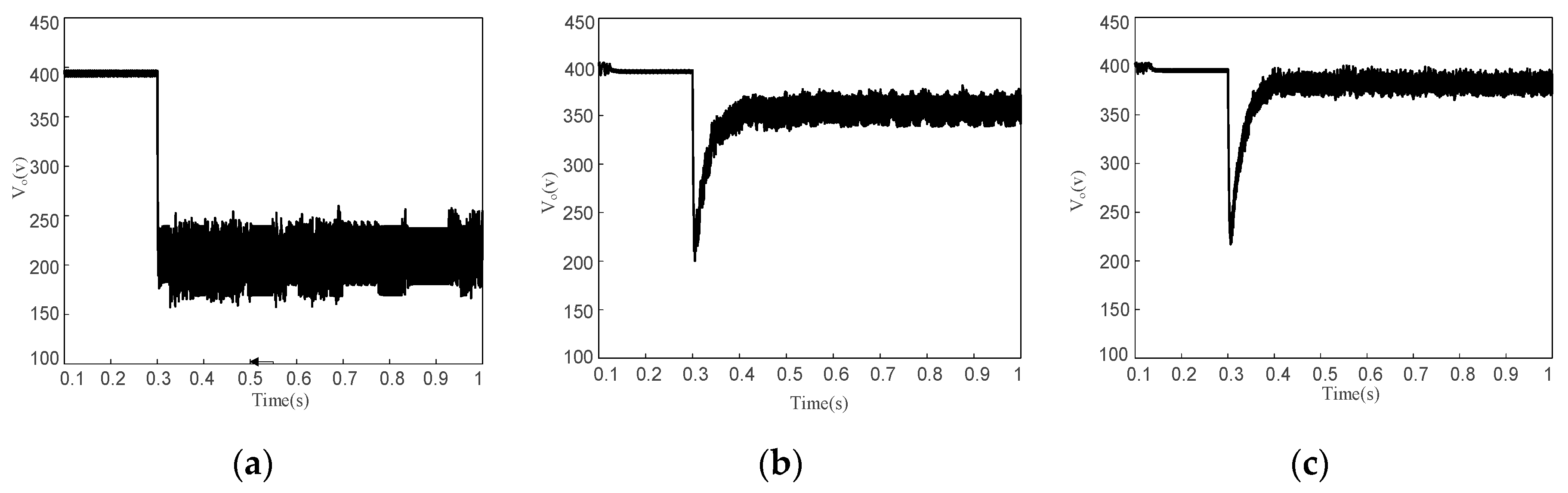
5.2. Validity Verification of Nonlinear Droop Control Strategy

The large signal stability criterion of the system under the nonlinear strategy is shown in Equation (32). The coefficient b of the quadratic polynomial still takes the linear droop coefficient (0.8 and 0.6), and the coefficient a should satisfy the inequality b-2ai > 0. When the power of the constant power load becomes 36,100 W, the system using the traditional linear droop control loses stability, as shown in Figure 9a; when the nonlinear droop control strategy is used, the waveform of the DC bus voltage is shown in Figure 9b,c.

According to Equation (25), the coefficients a1 and a2 of the two micro-sources in Figure 9b were 1.5 × 10⁻³ and 8.4 × 10⁻⁴, respectively. In Figure 9c, a1 and a2 are 2 × 10⁻³ and 1.25 × 10⁻³, respectively. As shown in Figure 9, the bus voltage drop in Figure 9c was smaller than that in Figure 9b at the steady state because the slope of the droop curve decreased as coefficient a increased, leading to the decline in the bus voltage drop. As for the large signal stability of the system, it was obvious that the system with the nonlinear droop control had better stability than the traditional linear droop controlled system, indicating that the method improved the system’s ability to resist large disturbances.

6. Conclusions

For DC microgrid systems with multiple micro-sources under droop control, large-signal stability analysis is difficult to quantify due to the existence of interactions between multiple closed-loops in the control system. In response to this situation, this paper simplified the large-signal model of the system through reasonable assumptions. The stability analysis was carried out by the mixed potential function method, the simple form of the large signal stability criterion was obtained by ignoring some integral terms, and the rationality of the simplifying step was analyzed. On this basis, a nonlinear droop control strategy was proposed to improve the system’s large signal stability. Finally, the validity of the large signal stability criterion and the effectiveness of nonlinear droop control strategy were verified by simulation.

However, there are still some important work to do in future research. First, a more detailed model of the system should be built considering the grid structure. Second, the influence of more parameters and other factors on system stability should be studied. Finally, it is important to understand the essential mechanisms of system stability and summarize a convenient research method with a wider scope of application.

References

1. Lasseter, R.H.; Eto, J.H.; Schenkman, B. CERTS microgrid laboratory test bed. IEEE Trans. Power Deliv. 2001, 26, 325–332. [Google Scholar] [CrossRef]
2. Zhang, Y.; Li, Y. Energy management strategy for supercapacitor in autonomous DC microgrid using virtual impedance. Appl. Power Electron. Conf. Expo. 2015, 725–730. [Google Scholar] [CrossRef]
3. Rana, M.M.; Xiang, W.; Wang, E. Smart grid state estimation and stabilization. Int. J. Electr. Power Energy Syst. 2018, 102, 152–159. [Google Scholar] [CrossRef]
4. Li, W.; Gu, Y.; Wang, Y.; Xiang, X.; He, X. Control Architecture and Hierarchy Division for Renewable Energy DC Microgrids. Autom. Electr. Power Syst. 2015, 39, 156–163. [Google Scholar]
5. Li, M.; Huang, W.; Tai, N.; Yu, M. Lyapunov-Based Large Signal Stability Assessment for VSG Controlled Inverter-Interfaced Distributed Generators. Energies 2018, 11, 2273. [Google Scholar] [CrossRef]
6. Wang, R.; Wu, Y.; He, G.; Lv, Y.; Du, J.; Li, Y. Impedance Modeling and Stability Analysis for Cascade System of Three-Phase PWM Rectifier and LLC Resonant Converter. Energies 2018, 11, 3050. [Google Scholar] [CrossRef]
7. Weinstein, M.I. Lyapunov stability of ground states of nonlinear dispersive evolution equations. Commun. Pure Appl. Math. 1986, 39, 51–67. [Google Scholar] [CrossRef]
8. Rivetta, C.H.; Emadi, A.; Williamson, G.A.; Jayabalan, R.; Fahimi, B. Analysis and control of a buck DC-DC converter operating with constant power load in sea and undersea vehicles. Ind. Appl. IEEE Trans. 2006, 42, 559–572. [Google Scholar] [CrossRef]
9. Rivetta, C.H.; Emadi, A.; Williamson, G.A. Large-signal analysis of a DC-DC buck power converter operating with constant power load. In Proceedings of the 29th Annual Conference of the IEEE Industrial Electronics Society, 2003, IECON’03, Roanoke, VA, USA, 2–6 November 2003. [Google Scholar] [CrossRef]
10. Marx, D.; Magne, P.; Nahid-Mobarakeh, B.; Pierfederici, S.; Davat, B. Large signal stability analysis tools in dc power systems with constant power loads and variable power loads—A review. IEEE Trans. Power Electron. 2012, 27, 1773–1787. [Google Scholar] [CrossRef]
11. Magne, P.; Marx, D.; Nahid-Mobarakeh, B.; Pierfederici, S. Large-Signal stabilization of a dc-link supplying a constant power load using a virtual capacitor: impact on the domain of attraction. IEEE Trans. Ind. Appl. 2012, 48, 878–887. [Google Scholar] [CrossRef]
12. Liu, X.; Zhou, Y.; Zhang, W. Large signal stability criteria for constant power loads with damped filters. Trans. China Electrotech. Soc. 2011, 26, 154–160. [Google Scholar]
13. Liu, X.; Zhou, Y.; Zhang, W.; Ma, S. Stability criteria for constant power loads with multistage filters. IEEE Trans. Veh. Technol. 2011, 60, 2042–2049. [Google Scholar] [CrossRef]
14. Tahim, A.P.N.; Pagano, D.J.; Lenz, E.; Stramosk, V. Modeling and stability analysis of islanded dc microgrids under droop control. IEEE Trans. Power Electron. 2015, 30, 4597–4607. [Google Scholar] [CrossRef]
15. Su, M.; Liu, Z.; Sun, Y.; Han, H.; Hou, X. Stability analysis and stabilization methods of dc microgrid with multiple parallel-connected dc–dc converters loaded by CPLs. IEEE Trans. Smart Grid 2017, 9, 132–142. [Google Scholar] [CrossRef]
16. Li, Z.; Kong, L.; Pei, W.; Ye, H.; Deng, W. Large-Disturbance stability analysis of droop-controlled dc microgrid based on mixed potential function. Power Syst. Technol. 2018, 42, 3725–3734. [Google Scholar]
17. Zhao, Z.; Hu, J.; Xue, H.; Huang, R.; Li, X.; Zhang, X. Large signal stability analysis of dc microgrid under droop control with constant power load. Chin. Autom. Congr. (CAC) 2017, 1046–1051. [Google Scholar] [CrossRef]
18. Brayton, R.K.; Moser, J.K. A theory of nonlinear networks. Q. Appl. Math. 1964, 22, 1–33. [Google Scholar] [CrossRef]
19. Weiss, L.; Mathis, W.; Trajkovic, L. A Generalization of Brayton-Moser’s Mixed Potential Function. IEEE Trans. Circuits Syst. Fundam. Theory Appl. 1998, 45, 423–427. [Google Scholar] [CrossRef]
20. Liang, H.; Zheng, C.; Gao, Y.; Li, P. Research on improved droop control strategy for microgrid. Proc CSEE 2017, 37, 4901–4910. [Google Scholar]
21. Liang, H.; Dong, Y.; Huang, Y.; Zheng, C.; Li, P. Modeling of multiple master–slave control under island microgrid and stability analysis based on control parameter configuration. Energies 2018, 11, 2223. [Google Scholar] [CrossRef]
Figure 1. System structure of a DC microgrid.
Energies 12 03186 g001
Figure 2. Equivalent circuit diagram of a DC microgrid.
Energies 12 03186 g002
Figure 3. Simplified equivalent diagram of the DC microgrid.
Energies 12 03186 g003
Figure 4. Diagram of improved droop curve.
Energies 12 03186 g004
Figure 5. Control block diagram of the proposed strategy.
Energies 12 03186 g005
Figure 6. Simulation model of the DC microgrid.
Energies 12 03186 g006
Figure 7. Waveforms of the DC bus voltage in case of (a) PCPL changes to 25,400 W; (b) PCPL changes to 34,300 W; (c) PCPL changes to 36,100 W.
Energies 12 03186 g007
Figure 8. Waveforms of DC bus voltage with (a) No.1 set of parameters; (b) No.2 set of parameters; (c) No.3 set of parameters; (d) No.4 set of parameters.
Energies 12 03186 g008
Figure 9. Waveforms of bus voltage with (a) Traditional Droop Control; (b) Nonlinear Droop Control with larger droop coefficients; (c) Nonlinear Droop Control with smaller droop coefficients.
Energies 12 03186 g009