Article

Numerical Study of Variable Camber Continuous Trailing Edge Flap at Off-Design Conditions

by
Mohammed Abdul Raheem
1,
Prasetyo Edi
2,
Amjad A. Pasha
1,*,
Mustafa M. Rahman
3 and
Khalid A. Juhany
1
1
Department of Aeronautical Engineering, King Abdulaziz University, Jeddah 21589, Saudi Arabia
2
Department of Aerospace Engineering, King Fahd University of Petroleum and Minerals, Dhahran 31261, Saudi Arabia
3
Mechanical Engineering Program, Physical Science and Engineering Division, King Abdullah University of Science & Technology, Thuwal 23955, Saudi Arabia
*
Author to whom correspondence should be addressed.
Energies 2019, 12(16), 3185; https://doi.org/10.3390/en12163185
Submission received: 25 May 2019 / Revised: 22 July 2019 / Accepted: 2 August 2019 / Published: 20 August 2019
(This article belongs to the Special Issue Modelling of Aerospace Vehicle Dynamics)

Abstract

:
Numerical simulations are performed to study the outboard airfoil of advanced technology regional aircraft (ATRA) wings with five different variable camber continuous trailing edge flap (VCCTEF) configurations. The computational study aims to improve the aerodynamic efficiency of the airfoil under cruise conditions. The design of outboard airfoil complies with the hybrid laminar flow control design criteria. This work is unique in terms of analysis of the effects of VCCTEF on the ATRA wing’s outboard airfoil during the off-design condition. The Reynolds–Averaged Navier–Stokes equations coupled with the Spalart-Allmaras turbulence model are employed to perform the simulations for the baseline case and VCCTEF configurations. The current computational study is performed at an altitude of 10 km with a cruise Mach number of 0.77 and a Reynolds number of 2.16 × 10⁷. Amongst all five configurations of VCCTEF airfoils studied, a flap having a parabolic profile (VCCTEF 123) configuration shows the maximum airfoil efficiency and resulted in an increase of 6.3% as compared to the baseline airfoil.

1. Introduction

The future growth of the aircraft industry depends on various environmental factors, such as air and noise pollution [1]. The fuel consumption of an aircraft is strongly dependent on its airfoil efficiency measured in terms of lift to drag (L/D) ratio. Increasing this efficiency is one of the methods for decreasing fuel consumption, thereby reducing harmful emissions [1]. It is evident in Figure 1 that “research, testing project design” represents 5% of the aircraft sale price which itself is 40% of direct operation cost (DOC). This estimate implies that “research, testing project design” contributes 2% (5% of 40%) of direct operation cost (DOC). The fuel accounts for 20% of DOC as illustrated in Figure 2 and a fuel savings of 10% implies 2% reduction in DOC [2]. Therefore, this study strives to increase the efficiency of airfoil.
The fuel consumption is strongly dependent on the aerodynamic efficiency [3] given by:
d W f ¯ = d η ¯
where η = L/D is aerodynamic efficiency, L is the lift force, D is the drag force, d η ¯ is the percentage change in η, and W f ¯ is the fuel consumption rate in terms of percentage.
It is observed from Equation (1) that the fuel consumption rate decreases with an increase in aerodynamic efficiency.
Range =   V C t L D l n W i n i t i a l W f i n a l
The Breguet–Range equation shows that aerodynamic efficiency must be maximum and the thrust specific fuel consumption (Ct) must be minimum, in other words, the fuel-efficiency must be maximum to attain the maximum aircraft range.
An increment in the L/D ratio can be achieved, either by increasing the lift force or by reducing the drag force. The high lift devices like slats, slots, and flaps are some of the effective techniques for increasing the lift [4]. However, an increment of the lift is inherently accompanied by the drag, so reducing the drag seems to be a better idea for increasing the L/D ratio.

Techniques for Increasing Aerodynamic Efficiency

In a subsonic transport aircraft, the majority of the drag is contributed by skin friction during the cruise condition [5,6,7]. The drag reduction can be obtained by suppressing the turbulent skin friction by manipulating boundary layer [8], using devices such as riblets [9] and large eddy break-up devices [10]. However, an increased cost of manufacturing and maintenance is a concern [6]. The vortex generators re-energize the boundary layer (by generating vortices) and delay the flow separation [11]. The drag reduction can also be achieved by altering the flow behavior by the use of additives such as particle, surfactant, bubble, and polymer solutions [12].
A reduction in the drag (by the aforementioned methods) especially the local skin friction drag reduction in the range of 5–30% is of considerable importance, but it is not as effective as laminar flow control (LFC), which results in 50–80% reduction in skin friction drag. The LFC by suction technique tends to delay the transition point, keeping the flow laminar for a certain portion of the wing. The natural laminar flow (NLF) technology changes the shape of the airfoil such that it moves the thickest point of the airfoil as aft as possible and reduces its thickness to the greatest feasible extent.
The hybrid laminar flow control (HLFC) has proved to be a significant development of LFC [13]. The advantages of the airfoil designed based on the HLFC criteria surpasses the limitations of NLF and LFC by suction (LFCS). In particular, the airfoil designed based on the HLFC criteria has a good design performance in the turbulent flow [13]. It also reduces the system complexity and cost as compared to the NLF and LFCS [14]. A drag reduction in the range of 10–11% is reached by the HLFC approach [15]. The practical use of HLFC requires that laminar flow is maintained through a range of cruise lift coefficients and Mach numbers. There can be a loss of laminar flow if there is a variation in lift coefficient and Mach number due to the change in the designed pressure distribution. A combination of HLFC and Variable Camber Wing (VCW) techniques suggested that the variable camber (flap deflection at a low angle of attack) can maintain the designed pressure distribution at off-design conditions, to obtain an optimum benefit [16].
The recent advances in aircraft structural materials have enabled the aerospace engineers to design the wings with greater stiffness (higher modulus of elasticity, E) while keeping the same load-carrying capacity. However, owing to the use of the stiffer wings, the aeroelastic interaction with forces and moments (generated due to the aerodynamics of the aircraft) results in the reduction of the aerodynamic efficiency. In order to overcome this aerodynamic problem, the wing surfaces must be shaped elastically during the cruise by active control of wing bending and twist [17]. The conventional flaps cannot be used to realize this concept; instead, a new type of flap system developed by NASA, i.e., the variable camber continuous trailing edge flap (VCCTEF) system, can be used. In comparison to the present flap system, the VCCTEF has the advantage of weight-reduction. This is because of the use of lightweight shape memory alloy (SMA) and an electric motor for actuation of its three-segment flap. The VCCTEF is developed for an airframe like the B757, a NASA Generic Transport Model (GTM). The VCCTEF uses a three-segment flap along the chord for varying camber. The cambered flap is expected to have a reduction in drag compared to the conventionally used single flap. Along the span, the flaps are divided into two-foot segments; this enables different flap settings at each flap along the span. Hence, the wing twist, or flexibility, is incorporated as a function of the span, resulting in a wing twist that varies according to the mission, thereby providing the best L/D ratio. The experimental studies show that the VCCTEF can achieve a drag reduction of up to 6.31% and an improvement in the L/D ratio up to 4.85% [18]. Hence, it is concluded that a combination of HLFC–VCCTEF seems to be more realizable in comparison to the HLFC–VCW. This combination is justified since the VCCTEF configuration can provide benefits such as reduced weight and active control of wing twist and bend compared to a conventional flap.

2. Present Work

The initial studies of VCCTEF have been conducted by deploying it on the airframe of the GTM wing. Edi et al. [16] reviewed the new technologies related to the wing design of civil–transport aircraft and had considered the combination of HLFC–VCW on the wing of advanced technology regional aircraft (ATRA) [19]. The present work reports the combination of HLFC–VCCTEF on ATRA wing’s outboard airfoil.

2.1. Wing of Advanced Technology Regional Aircraft (W-ATRA)

The W-ATRA wing is generated using three airfoils: (1) side of the body (SOB), (2) inboard (INB), and (3) outboard (KINK) airfoil. The SOB and the INB airfoil are designed proximate to the root of the wing. Figure 3a,b illustrate the wing thickness and twist distribution respectively along the wingspan. It is evident that the outboard airfoil is at 5.987 m from the fuselage centerline. The angle of incidence at this profile is 1.1° and the thickness to chord (t/c) ratio is 9.23%. The same t/c ratio is maintained until the wing tip; however, the angle of incidence varies linearly until −2°. The length of the outboard airfoil is 3587 mm at the wing break station. The angle of incidence of this airfoil varies from −2° to 1.1°.

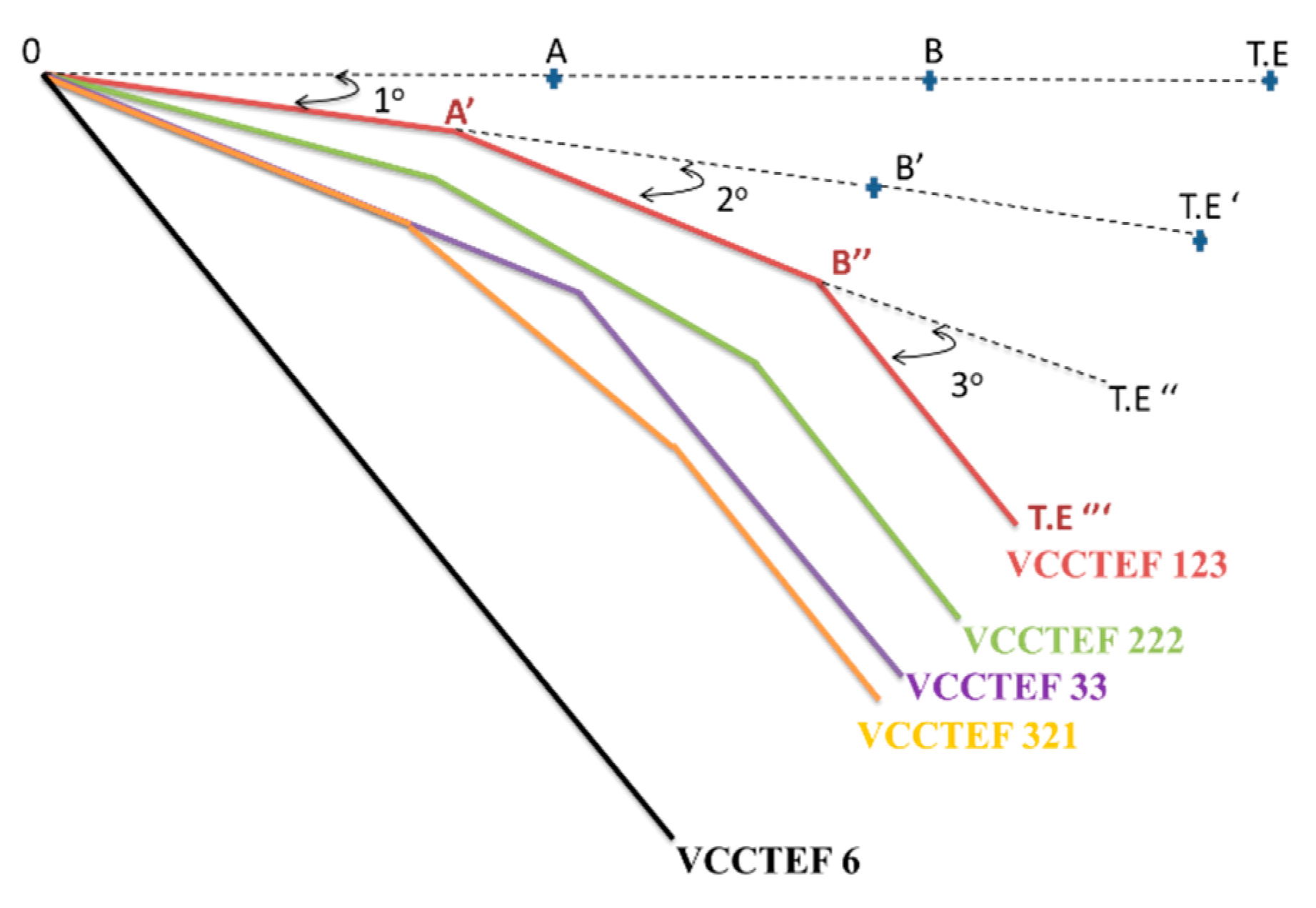
2.2. Combining VCCTEF with W-ATRA
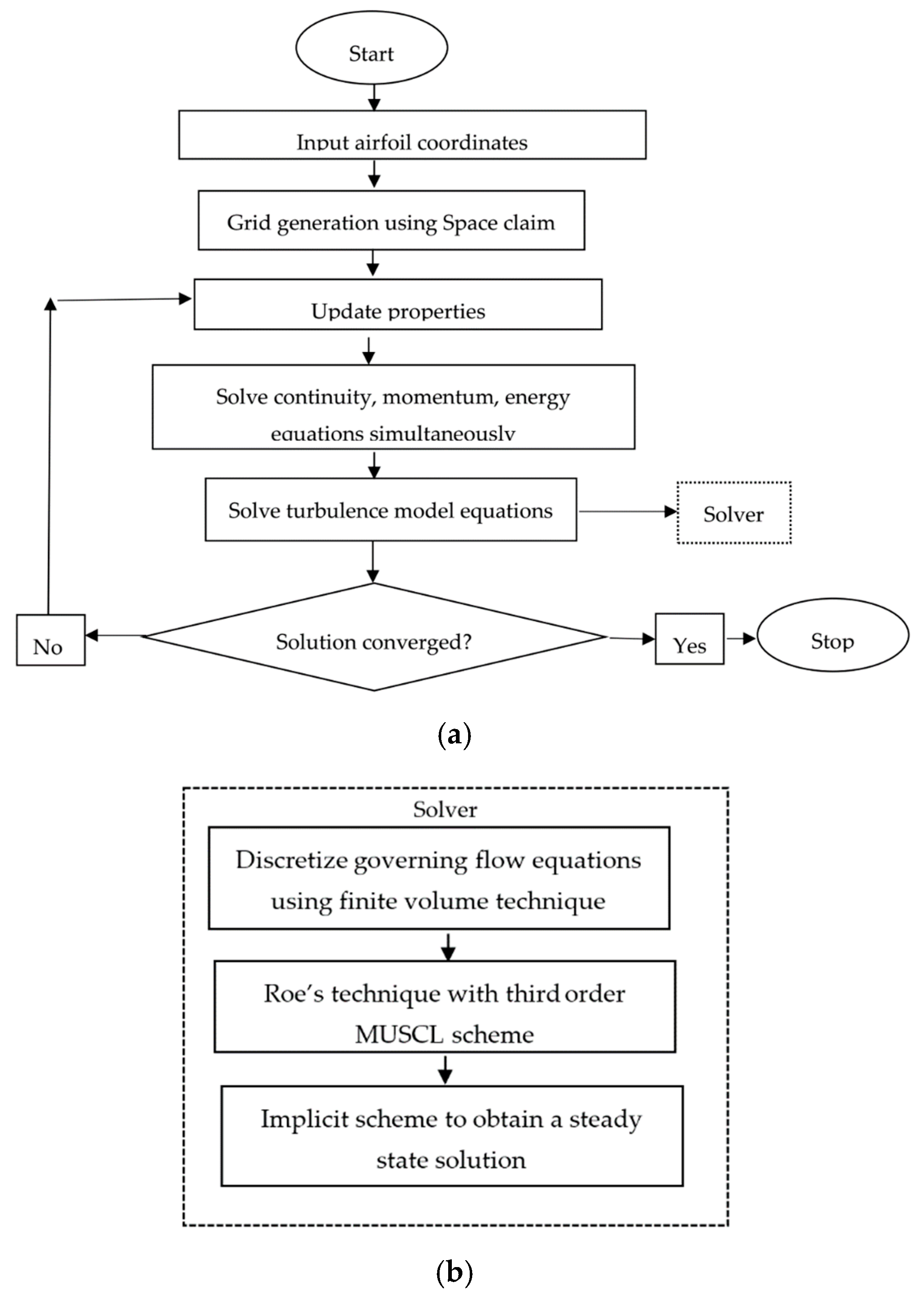
Given the discussion of the W-ATRA’s design features in the preceding section, there arises a question: what portion of the wing uses VCCTEF configuration? Is it to be used over the entire span or until a certain position along the span? In the NASA GTM wing, VCCTEF configuration is used after the wing break station (i.e., at the position where initial continuity in the wing is lost). An outboard/kink airfoil is used for making ATRA wing beyond the wing break station. Hence, in the present study, the VCCTEF configuration with an outboard airfoil alone is studied.
Table 1 shows various VCCTEF configurations on which simulations are conducted. The data in this table indicates that all the configurations for flaps (1–3) sum up to a value of 6°. For example, in VCCTEF 123, the sum of the angles is (1° + 2° + 3° = 6°). The reason for taking this angle of 6° is explained by Kaul et al. [20], who have studied these configurations computationally, but with another wing section of GTM wing. One of the objectives of the present work is to find any similarity with the previous work, hence the same angle of incidence is chosen for the current study.
Figure 4 shows the schematic of the three-segment flap each segment length is denoted by “cf”. Since the total flap length is 30% of chord (c), each cf is 10% of total chord length. The configuration of baseline airfoil is designed with no flap deflection, i.e., it has a zero deflection angle with respect to the horizontal line. The VCCTEF 123 indicates that there are three segments of the flap. The first segment is deflected at 1° from the horizontal line; the second segment is deflected at 2° from the first segment, and the third segment is deflected at 3° relative to the second segment (see Figure 5). The same jargon applies to the VCCTEF 222 and VCCTEF 321. The VCCTEF 33 is designed such that it has only two segments each deflected at 3° relative to the horizontal line and the first segment respectively. The VCCTEF 6 configuration is a variable camber flap with single deflection of 6° relative to the horizontal line.
Figure 6a shows the comparison of baseline coordinates with the various VCCTEF coordinates. Figure 6b shows the magnified view of the trailing edge, and it deflects in the order of VCCTEF 123, 222, 321, and 6, respectively. It is observed that the trailing edge of VCCTEF 321 and 33 almost coincide with each other.

3. Numerical Method

In the present work, the computational fluid dynamics (CFD) commercial software, ANSYS FLUENT V.17 is employed to perform the numerical simulations and its algorithm is illustrated in Figure 7. The airfoil coordinates in two–dimensions are normalized with the airfoil chord length. These coordinates are increased using the X–foil package to have a smoother profile of airfoil. The flow domain is divided into infinitesimal control volumes using Cartesian mesh. This mesh is generated using an in-built space claim package in ANSYS. The governing equations of continuity, momentum, and energy are solved simultaneously by using the density-based solver. The turbulence model equation is solved by using the formerly updated values of flow variables such as velocity, pressure, and temperature. The standard one-equation Spalart-Allmaras (SA) turbulence model is used to calculate the eddy viscosity [21]. The linearization of the coupled continuity, momentum, and energy equations produce a system of equations with unknown properties such as pressure, velocities, temperature and turbulent eddy viscosity. The inviscid flux terms are computed using Roe’s flux-differencing splitting method using 3rd order MUSCL scheme [22]. The implicit lower-upper symmetric Gauss-Seidel approach is used to advance the solution in time for all the variables in the control volumes to reach the steady-state solution. A Courant–Friedrichs–Lewy (CFL) number of 0.7 is used to achieve a converged solution. All the simulations are initialized with a constant free-stream temperature, pressure, and velocities. It is assumed that the air obeys an ideal gas law and the value of viscosity is adjusted to match the desired free stream Reynolds number (Re). The computations are stopped when the mass residual is reduced to an order of magnitude of six.

4. Results and Discussion
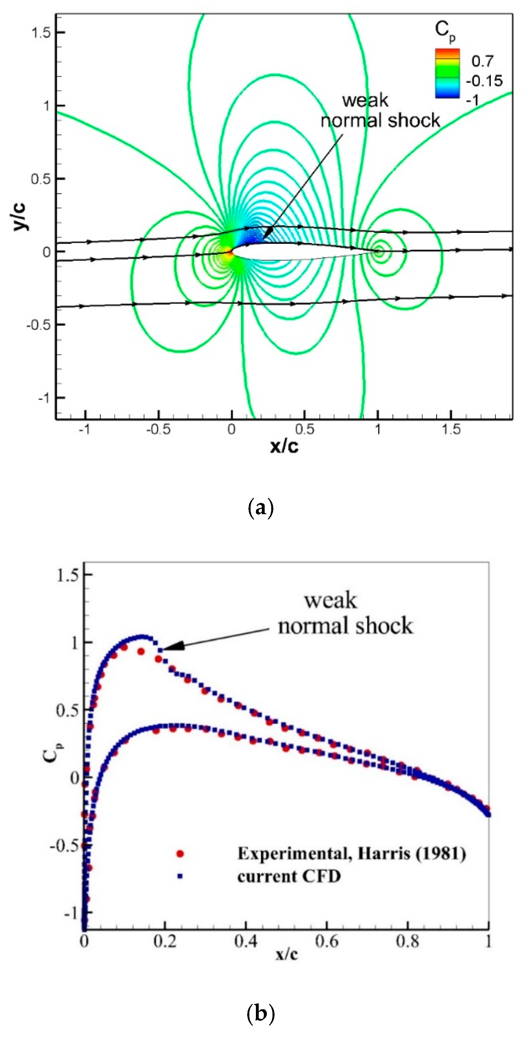
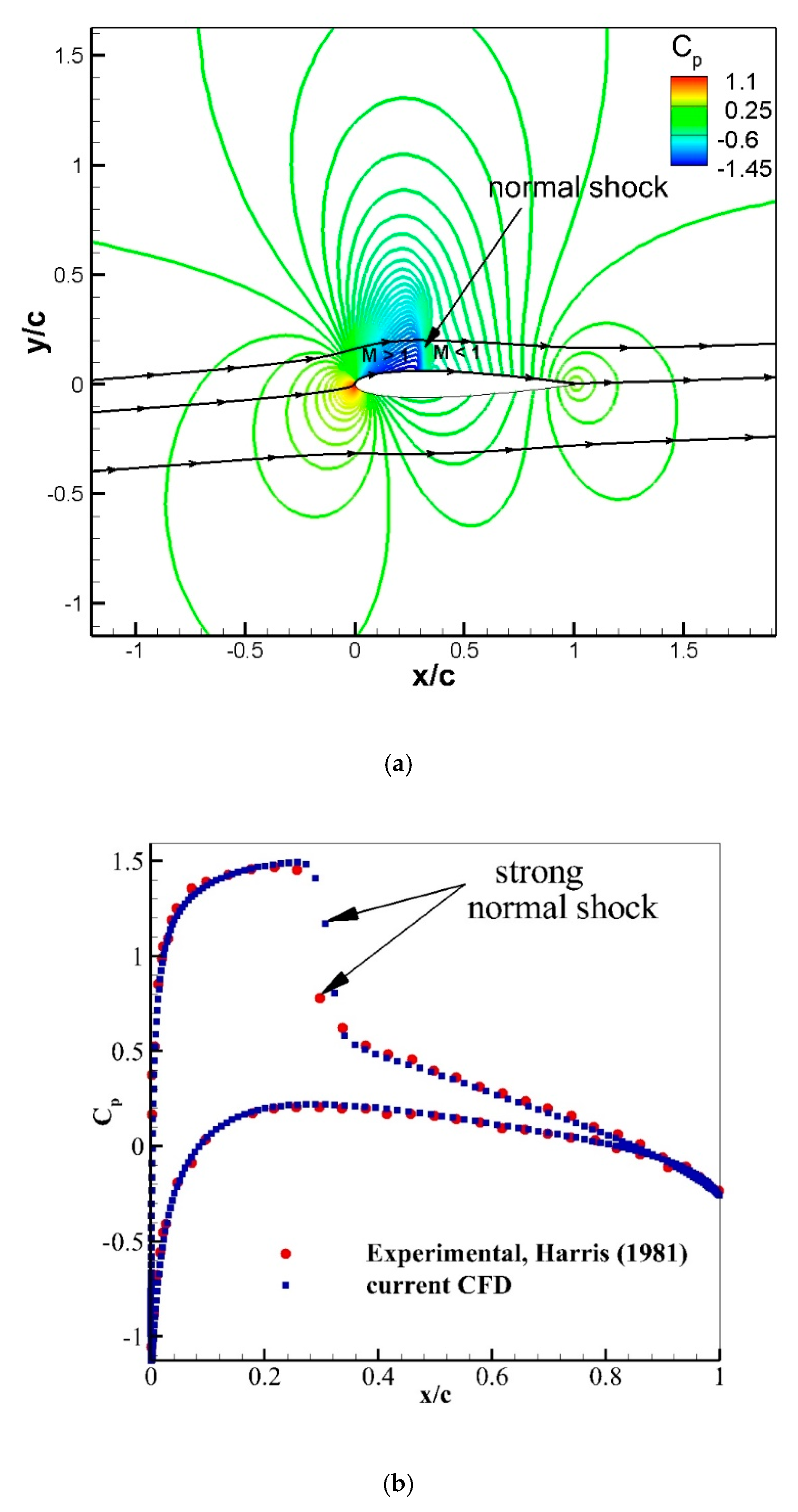
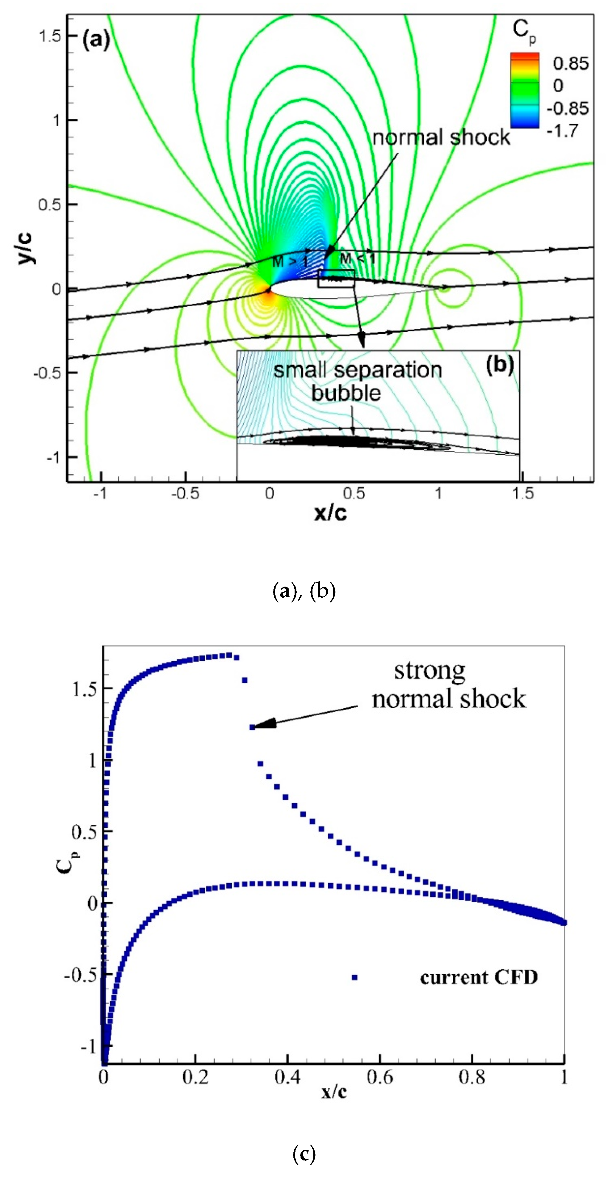
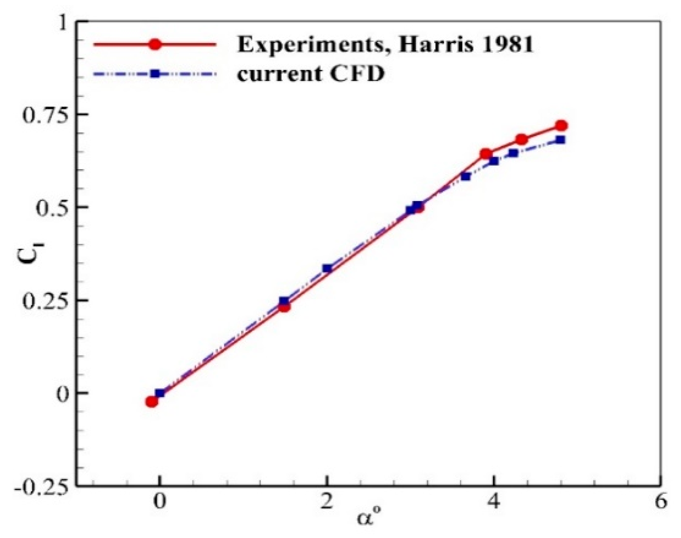
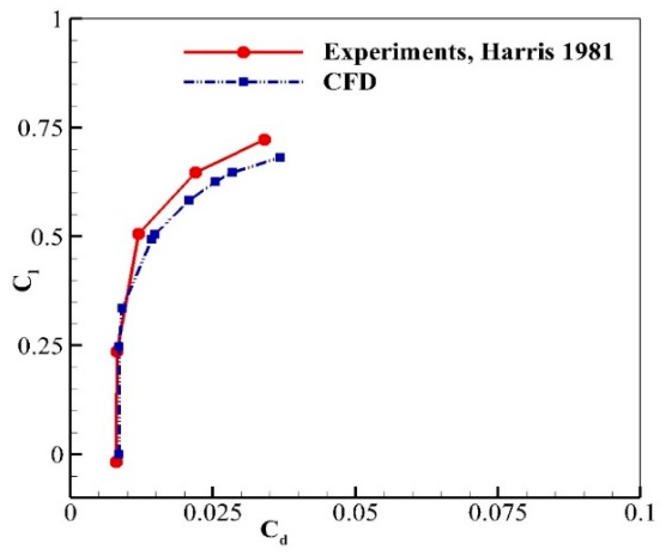
4.1. Validation

The flow over the NACA0012 airfoil is computed, and the results are compared to the available experimental data [23] for the validation at free stream transonic Mach number and Reynolds number of 0.7 and 9 × 10⁶. The C–grid with 1122 × 200 points is generated with flow domain extending up to 25 chord length. The flow is computed at different angles of attack varying from 0° to 4.8°. The experiments showed a stall at an angle of attack of 5°. The computed coefficient of pressure contours and surface pressure distributions are shown in Figure 8, Figure 9 and Figure 10 for the angle of attack = 1.5°, 3.1°, and 4.8° respectively and compared to the experiments [23]. A weak normal shock is formed on the upper surface of the airfoil and is marked in Figure 8a. The computed surface pressure coefficient matches with the experimental data on the upper and the lower airfoil surfaces (see Figure 8b), however on the upper surface in the regions near to x/c = 0.16, CFD data shows higher values than the experiments. This normal shock is absent in the experiments because of the three-dimensional (3–D) relieving effect. In a two-dimensional (2–D) computational flow, sharp gradients of the normal shock wave are formed. The computed Cp contour shows that the normal shock location (see Figure 9a) is observed in the downstream flow direction in comparison to the experimental data. Figure 9b illustrates that the CFD results are in a good agreement with the experimental data with a small deviation of Cp at x/c = 0.28 on the upper surface. An increase in the angle of attack results in a stronger normal shock on the upper surface, as shown in Figure 10a by flow contours of the coefficient of pressure. Figure 10b depicts that an adverse pressure gradient across the normal shock wave results in flow separation. Figure 10c illustrates that the highest jump in surface Cp across the shock is observed at x/c = 0.32.
The computed Cl variation with angle of attack for the NACA0012 airfoil at Mach = 0.7 and Re = 9 × 10⁶ is compared with the experiments [23] in Figure 11. The current computed Cl agrees well with experimental data up to 4° angle of attack and beyond this angle, the CFD results show 5% fewer values than experiments. Figure 12 shows a polar drag plot for the NACA0012 airfoil. The CFD results match with experiments for a lower angle of attack up to 2° and show a maximum deviation of 7% at higher angles. This difference can be attributed to the fact that the experiment fixed the transition location around 5 percent of the chord from the leading edge, while the present computations are carried out with a fully turbulent incoming flow with SA turbulence model. The second reason in deviation of CFD and experiments is that the normal shock is unsteady in nature when it interacts with the boundary layer on the airfoil surface. This normal shock–boundary-layer interaction is one of the sources of flow unsteadiness. The modelling of this flow unsteadiness and implementing in the turbulence model can improve the separation bubble size, and hence can improve the computed shock location. This unsteadiness is not modelled by the current SA model and therefore gives an error in the Cd and Cl calculations. The CFD results will be improved in our future studies by using advanced SA and k-ω turbulence models, which accounts for this unsteadiness [24,25,26,27].

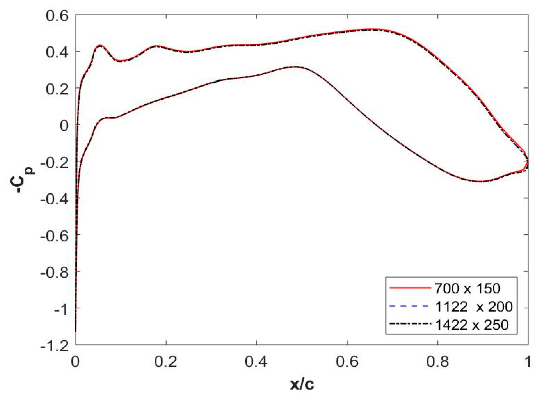
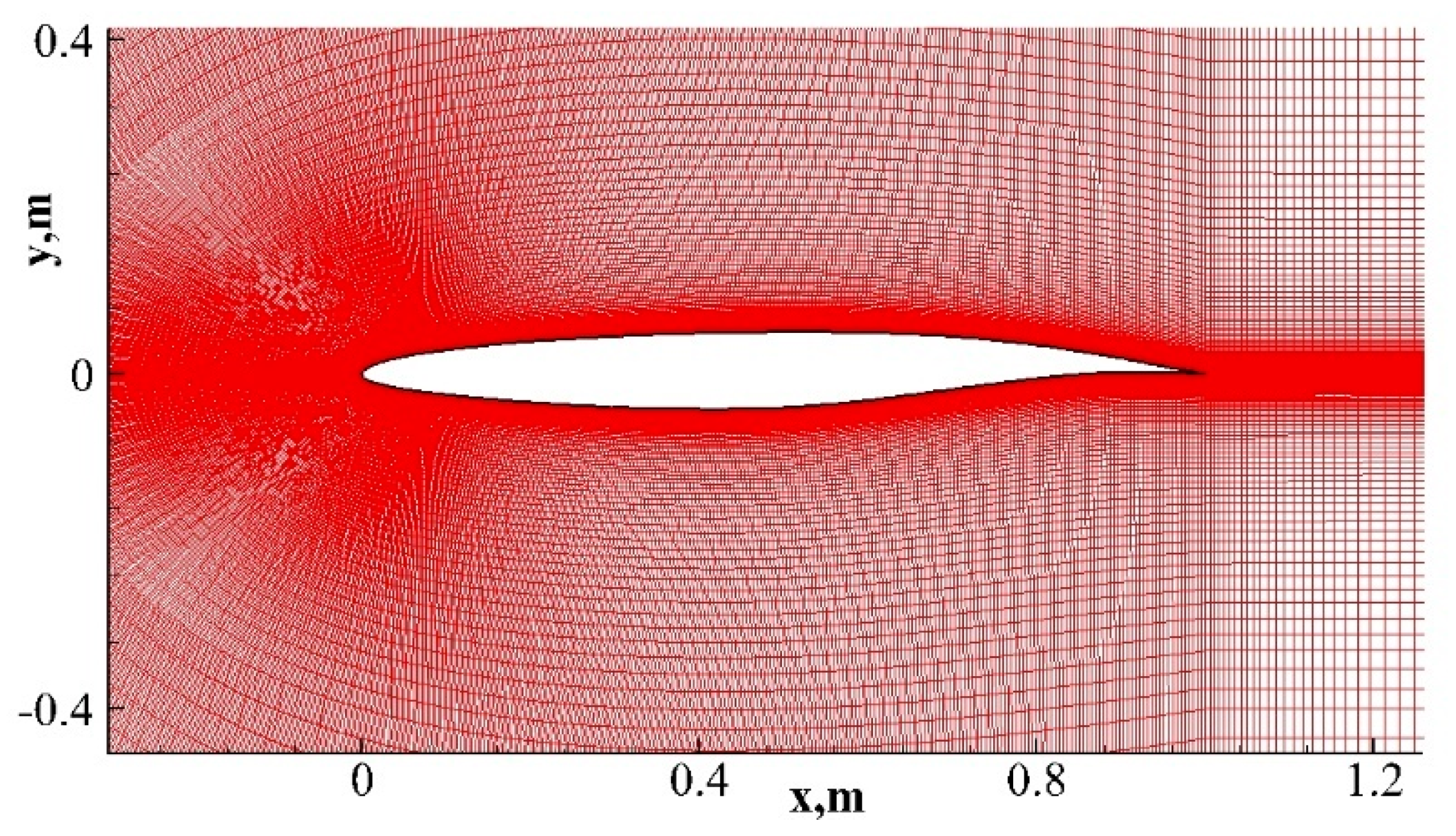
4.2. Grid Independence Study (Baseline)

A grid independence study is done by taking three different C–grids of 700 × 150, 1122 × 200 and 1422 × 200, as shown in Figure 13. It is observed that the variation of surface pressure coefficient overlaps with each other for these grids (see Figure 13). The near-wall distance of 1.6 × 10⁻³ m is taken and the value of y+ is less than 1. In the current study, the grid size of 1122 × 200 is used to reduce the numerical errors [22]. The number of grid points around the airfoil is 922 points. The same grid is used in the validation of NACA0012 airfoil in the former simulations. Figure 14 shows the grid around the baseline airfoil.

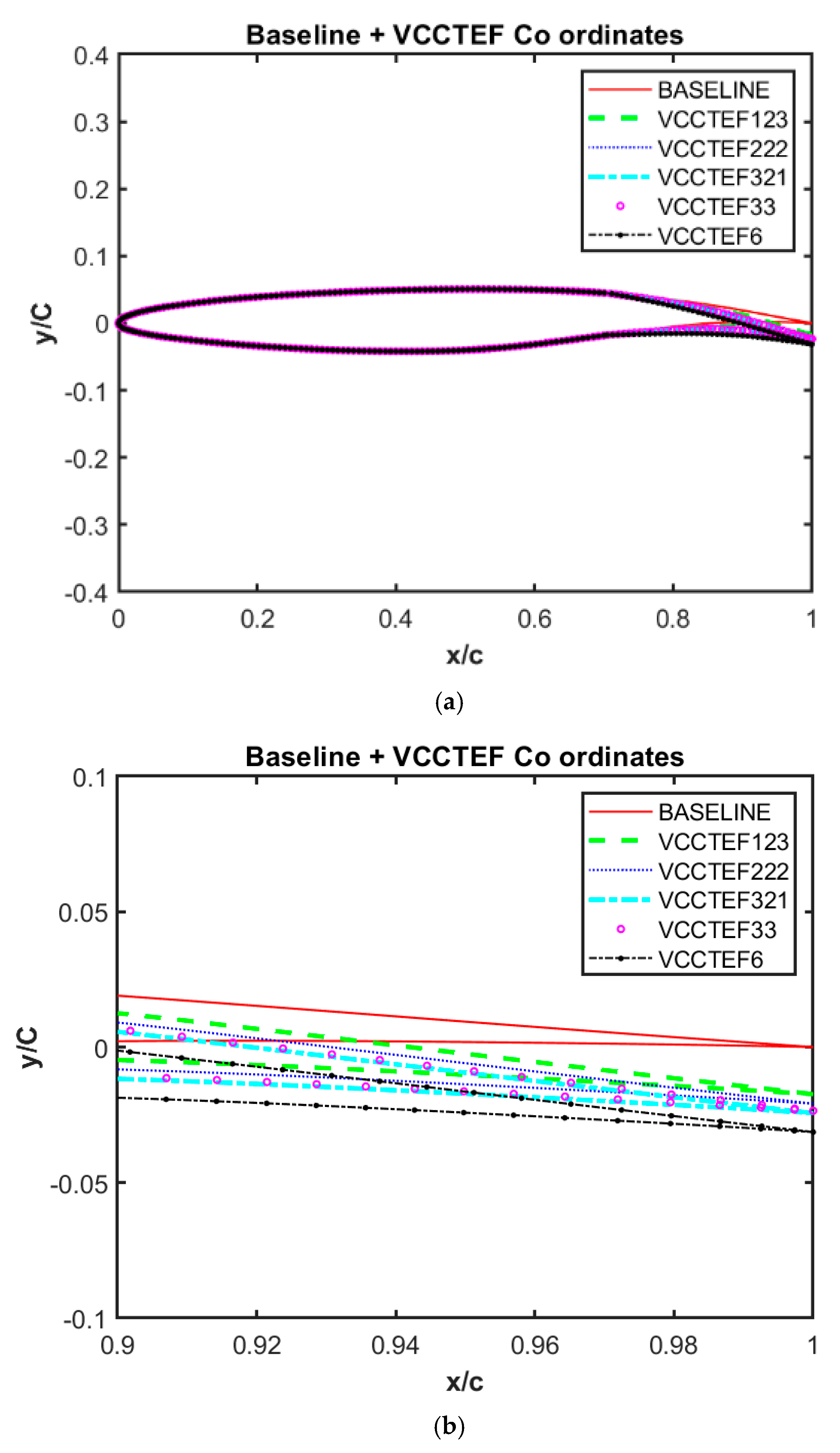
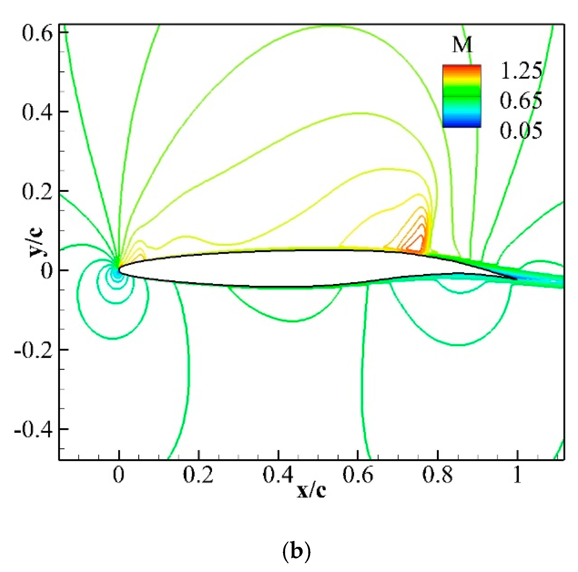
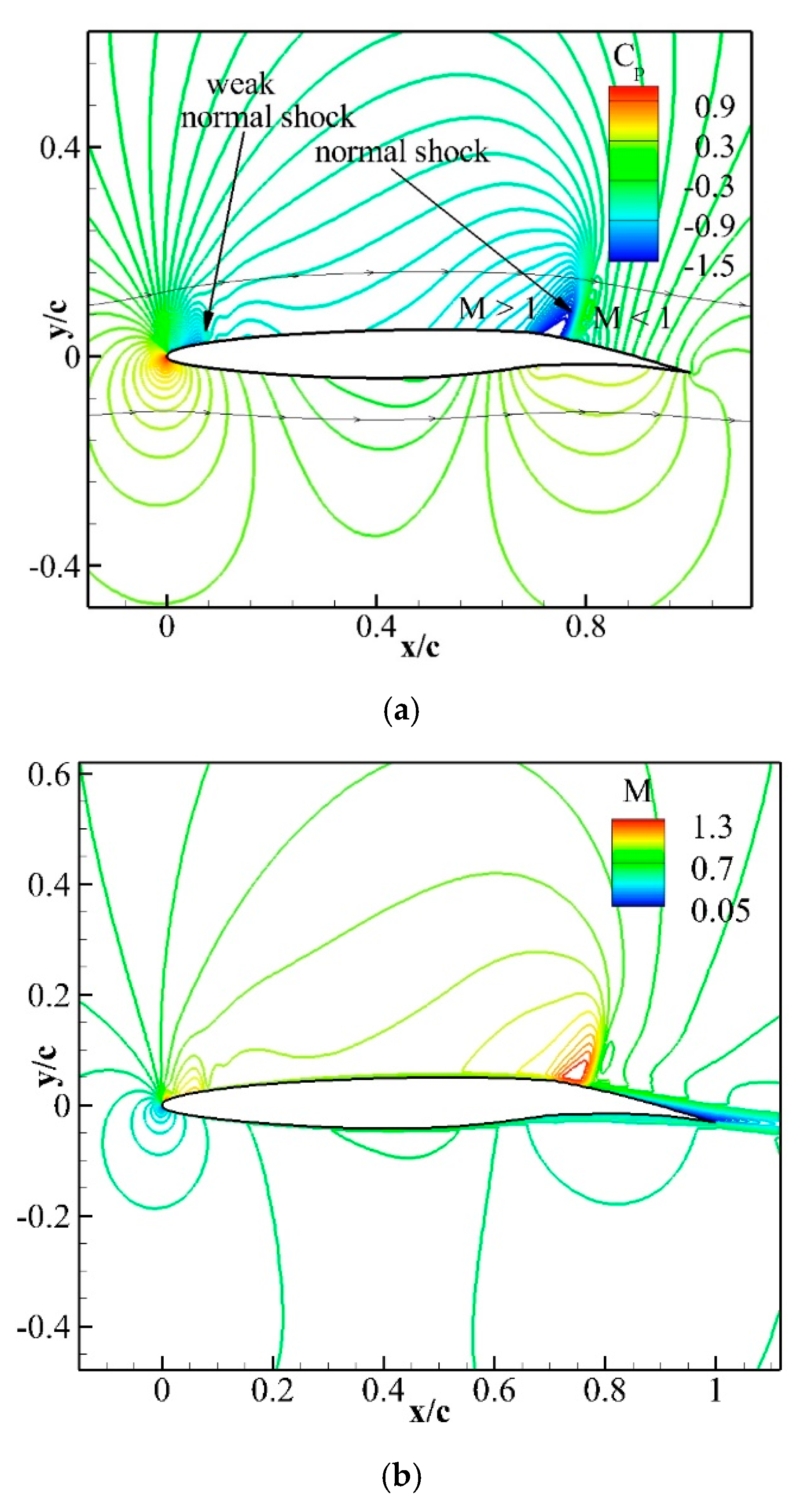
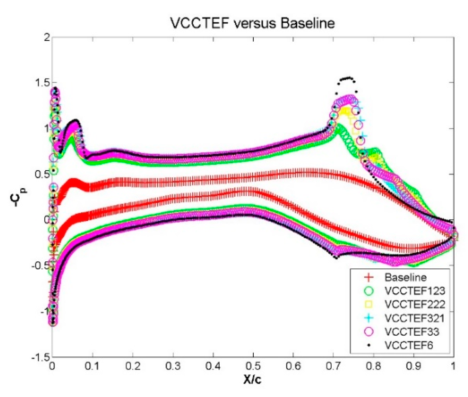
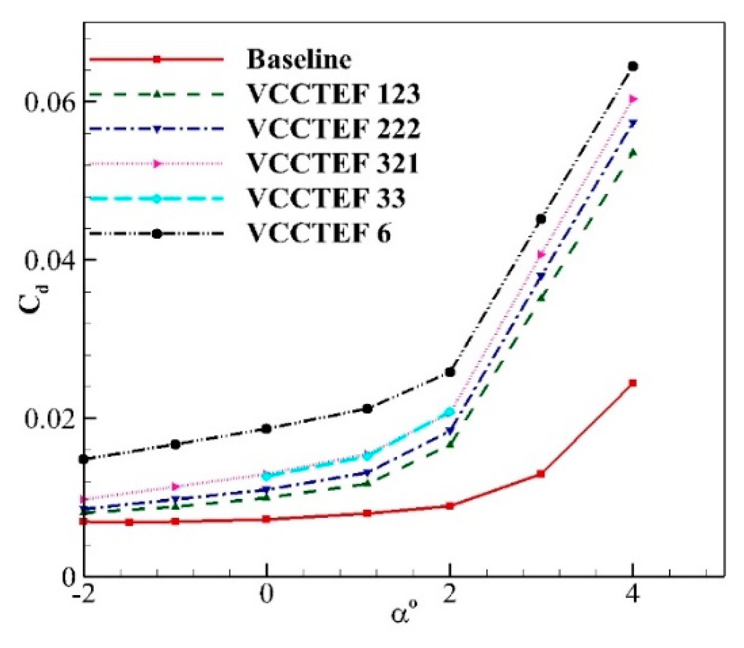
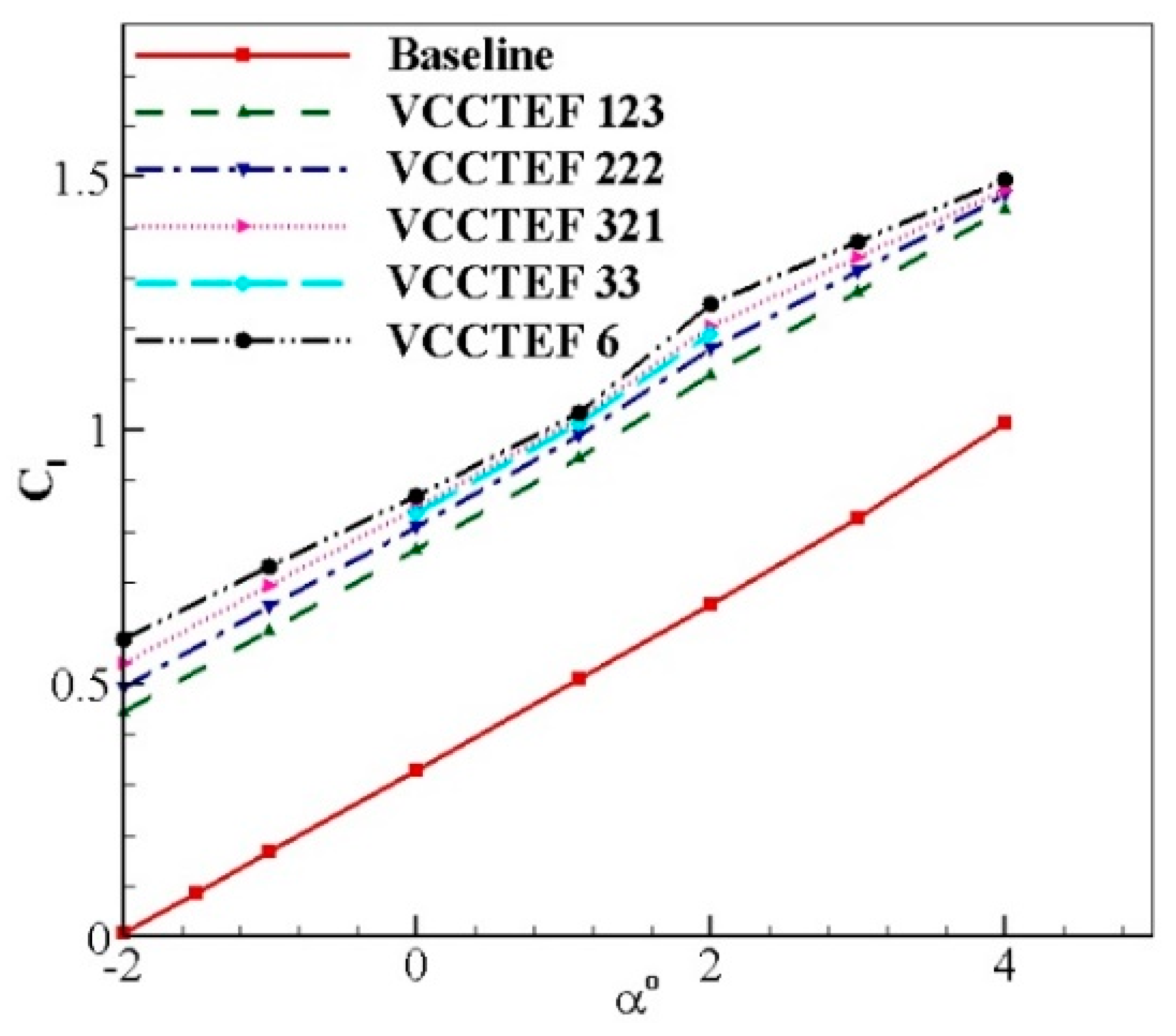
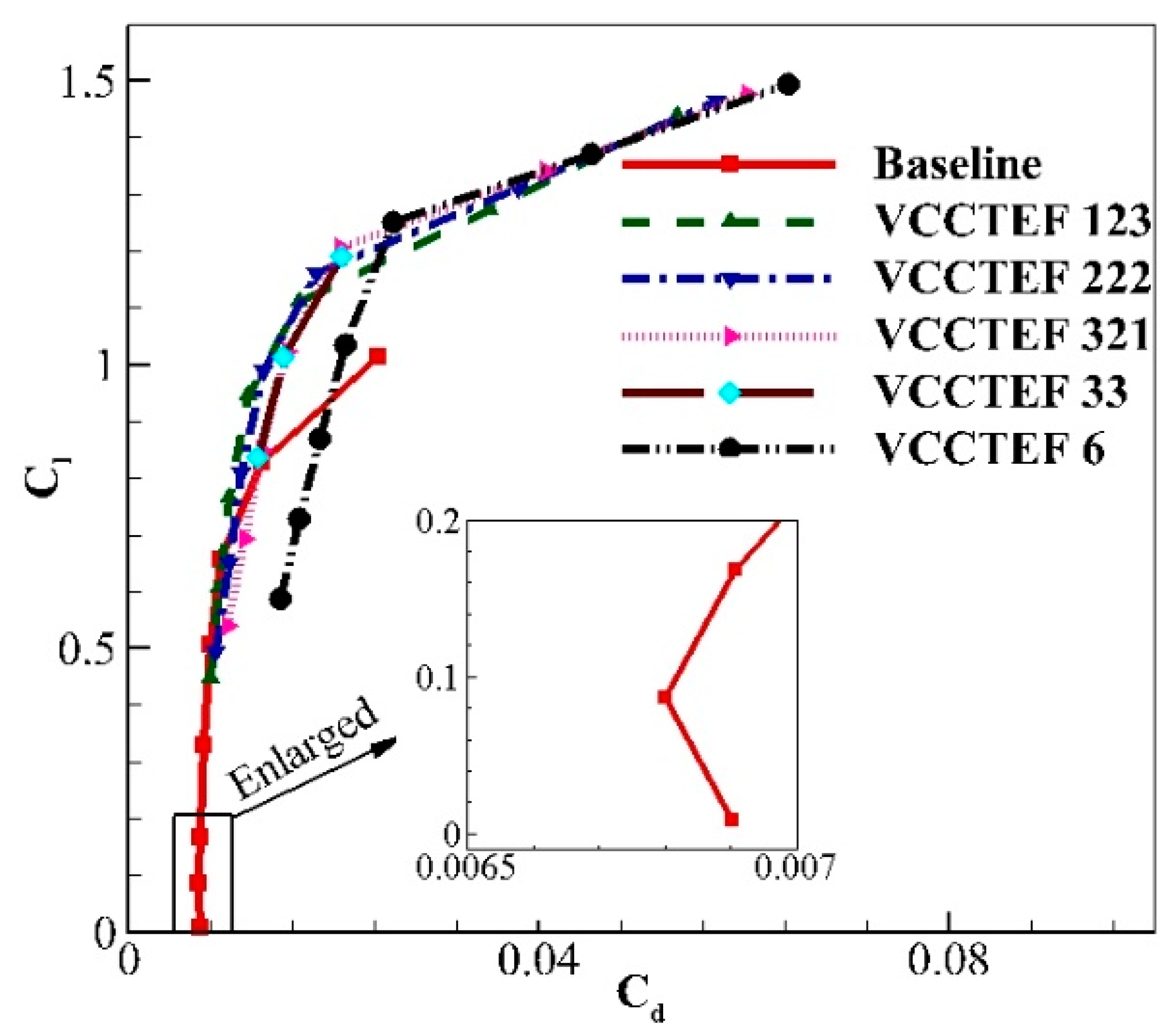
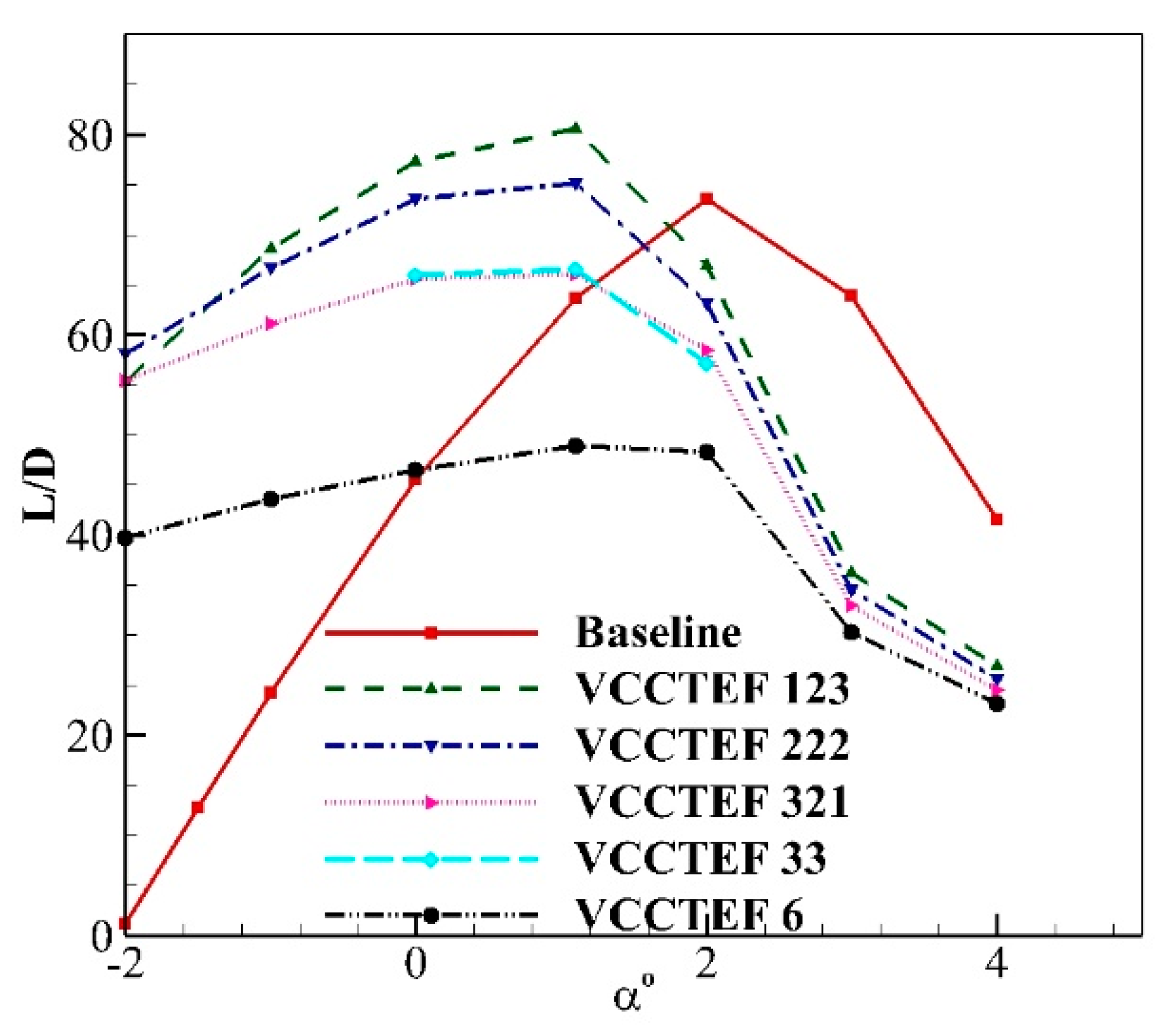
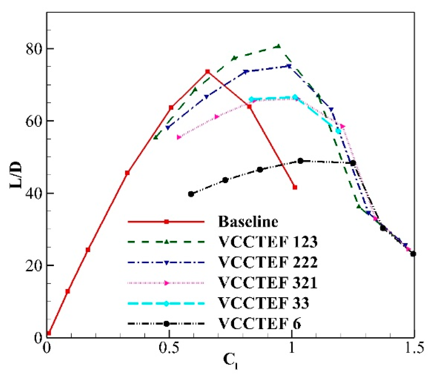
4.3. VCCTEF Simulations

The computations of 2–D fully turbulent flows are performed on the outboard airfoil of ATRA wing to explore the effects of various VCCTEF configurations on L/D ratio. The focus of the work is to select the most aerodynamically efficient VCCTEF configuration in comparison to the baseline airfoil. The number of coordinates of the outboard airfoil is increased to 300 points by using Xfoil software [28]. The numerical simulations are performed at a free-stream Mach number of 0.7 and free-stream Reynolds number of 21.6 × 10⁶. Since the aircraft wing is swept back at an angle of 25°, the actual Mach number over the aircraft’s wing would be 0.77 [29]. The free stream pressure and temperature corresponding to an altitude of 10 km are assumed to be p = 26,500 Pa and T = 223 K. In order to match the desired Re the viscosity is adjusted to a value of 1.44 × 10⁻⁵ Pa-s.
The coefficient of pressure and the Mach contour plots of the baseline and various VCCTEF configurations at a zero angle of attack are illustrated in Figure 15, Figure 16, Figure 17, Figure 18, Figure 19 and Figure 20. As the deflection of trailing edge increases (see Figure 6b) the normal shock intensity on the top surface of these airfoils also increases in the same order of deflection and are marked in the respective contours of the coefficient of pressure. The maximum Mach number on the upper surface of the airfoil, near the first hinge point, also increases in the same order.
The baseline pressure coefficient plot is compared at a zero angle of attack in Figure 21 with other VCCTEF configurations. The strength of normal shock formation at x/c ≈ 0.70 on the top surface of airfoil increases in the order of trailing edge deflection. The strength of the shock can be observed with an increase of bump at x/c ≈ 0.70 and is consistent with the flow physics contours of normal shock formation seen in Figure 15, Figure 16, Figure 17, Figure 18, Figure 19 and Figure 20. The flow expands before the shock, which can be observed by a decrease of pressure before the shock. Along with the strength of the shock, the flow expansion tendency also increases in the order of trailing deflection. It may be noted that the airfoil is designed to have an initial peak pressure near the leading edge [16] on the upper surface of the airfoil, as observed in Figure 21. However, this initial pressure peak proximate to the leading edge is amplified in the various VCCTEF configurations.
The VCCTEF 6 configuration is showing the highest level of drag compared to other configurations at any given angle of attack (see Figure 22). Among the five configurations of VCCTEF, the lowest drag is of VCCTEF 123. It is worth noting that VCCTEF 321 and 33 almost coincide with each other. The study of the variation in the Cd with various angle of attack is important for initial assessment of the VCCTEF configurations before the computations of the 3–D geometry begins. All the VCCTEF configurations result in an increase in the lift coefficient in comparison to the baseline airfoil (as observed in Figure 23) with the VCCTEF 6 showing the highest value at each angle of attack.
The polar drag comparison of baseline and other VCCTEF configurations can be seen in Figure 24. The minimum drag for the baseline airfoil is approximately equal to 0.0068 at Cl ≈ 0.1, whereas the parasite drag or the zero-lift drag is approximately equal to 0.0069. Almost all the VCCTEF configurations appear to have a similar minimum drag point. Among all the configurations, only the VCCTEF 6 configuration tends to have a relatively higher drag at its minimum drag position. The highest Cl that is achieved by any VCCTEF configuration is accompanied by an increase in drag as compared to the baseline airfoil.
The L/D value of all the VCCTEF configurations (except VCCTEF 6) is better than the baseline configuration for the angle of attack in the range of −2° to 1° (as seen in Figure 25). However, beyond 1.5°, no configuration outperforms the baseline.
It is evident from Figure 25 that VCCTEF 123 results in the best L/D ratio of 80 at α = 1.1°. The baseline case indicates better performance at α = 2° with L/D ≈ 75. The VCCTEF 222 airfoil shows a similar L/D but at α = 1°.
Figure 26 shows the variation of L/D with Cl; here it is seen that beyond the Cl ≈ 0.7, VCCTEF 123 and 222 perform better than baseline. The best performance in the cruise is given by the VCCTEF 123 with baseline and 222 being close in respective order. At Cl ≈ 0.6, which is the design lift coefficient of the baseline, it has the best aerodynamic efficiency.
Amongst the various VCCTEF configurations, the parabolic arc chamber (VCCTEF 123) has lesser shock intensity at the first hinge position; this is similar to the results of Kaul et al. [20]. All the VCCTEF configurations have better aerodynamic efficiency between −2° and 1.1° than baseline airfoil except for the single flap segment VCCTEF 6 configuration which underperforms relative to the baseline case beyond 0°.
Although the study has successfully demonstrated the efficient configuration of the airfoil, the current investigation of the SA model is not explicitly designed to do time-resolved simulation. Further analysis investigating these simulations cases with LES model [30] would help us to establish a greater degree of accuracy on this present study. Another interesting possible area of future research would be to investigate the aerodynamic performance of these airfoils in the atmosphere with particles. Airfoils can experience such dispersed flow of particles of varying size due to sandy desert environments [31]. Furthermore, research investigating these particulate flows would help analyze the airfoil efficiency in the dusty environment.

5. Conclusions

The airfoil used for the present study was an outboard airfoil of the wing of advanced technology regional aircraft (W-ATRA), which extends from wing break station to the tip. The airfoil has a chord length of 3587 mm (141.2205 inches). The variable camber continuous trailing edge flap (VCCTEF) overall flap chord is 30% of airfoil length, measured from the first hinge line. The simulations of the baseline and various VCCTEF configurations were performed using the fully turbulent Spalart-Allmaras model. The results identified the most aerodynamic efficient VCCTEF configuration amongst the various tested configurations. The VCCTEF 123 showed the best lift to drag ratio of 80 at an angle of attack equal to 1.1°. The SA model predicted an increase in the lift as well as drag as the angle of attack increases, this is due to the increment in the camber and the pressure component of the drag force respectively. The VCCTEF 123 configuration resulted in an approximately 6.3% increment in the lift to drag ratio as compared to the baseline case.
The VCCTEF airfoil was designed to have weak shocks near the leading edge. Upon neglecting the effect of weaker shocks near the leading edge, all the configurations (including baseline) show a favorable pressure gradient up to 65% of the chord at an angle of attack of 0° which is good for application of HLFC. In addition, all the VCCTEF configurations showed the shock formation at hinge positions with VCCTEF 6 having a strong shock. The VCCTEF 123, with a parabolic arc angle configuration, showed better performance than all configurations.
The three-dimensional CFD results tend to produce weak shocks on the surface of the airfoil in comparison to the two-dimensional CFD results. These two-dimensional effects may be absent in the experimental work. This is because the two-dimensional flow having sharp gradients due to shocks can be relieved in three-dimensional flow by variation of pressure gradient due to the crossflow. This change in properties in three-dimensional flow is denominated as a relief effect. Our future work is directed to perform the three-dimensional simulations to study the relief effect on the drag and lift of VCCTEF airfoils.

Author Contributions

Conceptualization, M.A.R., and P.E.; software, M.A.R., A.A.P. and P.E.; writing, review and editing, M.A.R., A.A.P. and M.M.R.; supervision, P.E., A.A.P., and K.A.J.; funding acquisition, K.A.J., M.M.R., and A.A.P.

Funding

This article was funded by the Deanship of Scientific Research (DSR) at King Abdulaziz University, Jeddah. The authors, therefore, acknowledge with thanks DSR for technical and financial support.

Acknowledgments

The authors would like to thank the Dean of Engineering and High-Performance Computing Centre (Aziz Supercomputer) (http://hpc.kau.edu.sa) for extending facilities to perform numerical simulations. We would like to thank Ahmed Z. Al-Garni from the Department of Aerospace Engineering, King Fahd University of Petroleum and Minerals and Rached Ben-Mansour from the Department of Mechanical Engineering, King Fahd University of Petroleum and Minerals for the help during the CFD simulations.

Conflicts of Interest

The authors declare no conflict of interest.

References

  1. Green, J.E. Civil aviation and the environmental challenge. Aeronaut. J. 2003, 107, 281–300. [Google Scholar]
  2. Marec, J.P. Drag Reduction: A Major Task for Research. In Proceedings of the CEAS/DragNet European Drag Reduction Conference, Potsdam, Germany, 19–21 June 2000; pp. 17–28. [Google Scholar]
  3. Bolonkin, A.; Gilyard, G.B. Estimated Benefits of Variable-Geometry Wing Camber Control for Transport Aircraft. NASA/TM-1999-206586; 1999. Available online: https://ntrs.nasa.gov/archive/nasa/casi.ntrs.nasa.gov/19990090019.pdf (accessed on 3 August 2019).
  4. Van Dam, C.P. The aerodynamic design of multi-element high-lift systems for transport airplanes. Prog. Aerosp. Sci. 2002, 38, 101–144. [Google Scholar] [CrossRef] [Green Version]
  5. Thibert, J.J.; Reneaux, J.; Schmitt, V. ON-ERA activities in drag Reduction. In Proceedings of the 17th Congress of the International Council of the Aeronautical Sciences, Stockholm, Sweden, 9–14 September 1990; Volume 17, pp. 1053–1064. [Google Scholar]
  6. Jahanmiri, M. Aircraft Drag Reduction: An Overview; Chalmers University of Technology: Gothenburg, Sweden, 2011; Available online: http://publications.lib.chalmers.se/records/fulltext/137214.pdf (accessed on 3 August 2019).
  7. Neittaanmäki, P.; Rossi, T.; Korotov, S.; Oñate, E.; Périaux, J.; Knörzer, D. Overview on drag reduction technologies for civil transport aircraft. In Proceedings of the European Congress on Computational Methods in Applied Sciences and Engineering (ECCOMAS), Jyväskylä, Finland, 24–28 July 2004; pp. 24–28. [Google Scholar]
  8. Slooff, J.W. Subsonic Transport Aircraft-New Challenges and Opportunities for Aerodynamic Research; The 36th Lanchester Lecture; Royal Aeronautical Society: London, UK, 1996. [Google Scholar]
  9. Sareen, A.; Deters, R.W.; Henry, S.P.; Selig, M.S. Drag reduction using riblet film applied to airfoils for wind turbines. J. Sol. Energy Eng. 2014, 136, 21007. [Google Scholar] [CrossRef]
  10. Anders, J.; Watson, R. Airfoil large-eddy breakup devices for turbulent drag reduction. In Proceedings of the Shear Flow Control Conference, Boulder, CO, USA, 12–14 March 1985; p. 520. [Google Scholar]
  11. Gao, L.; Zhang, H.; Liu, Y.; Han, S. Effects of vortex generators on a blunt trailing-edge airfoil for wind turbines. Renew. Energy 2015, 76, 303–311. [Google Scholar] [CrossRef]
  12. Zheng, X.F.; Yan, Y.Y. A Biomimetic Smart Control of Viscous Drag Reduction. Adv. Nat. Sci. 2010, 3, 139–151. [Google Scholar]
  13. Joslin, R.D. Aircraft laminar flow control. Annu. Rev. Fluid Mech. 1998, 30, 1–29. [Google Scholar] [CrossRef]
  14. Braslow, A.L. A History of Suction-Type Laminar-Flow Control with Emphasis on Flight Research; Monogr. Aerosp. Hist. Number 13; NASA: Washington, DC, USA, 1999.
  15. Boeing Commercial Airline Co. Hybrid Laminar Flow Control Study Final Technical Report NASA CR 165930. 1982. Available online: https://ntrs.nasa.gov/archive/nasa/casi.ntrs.nasa.gov/19850002625.pdf (accessed on 3 August 2019).
  16. Edi, P.; Fielding, J.P. Civil-Transport Wing Design Concept Exploiting New Technologies. J. Aircr. 2006, 43, 932–940. [Google Scholar] [CrossRef]
  17. Nguyen, N. Elastically Shaped Future Air Vehicle Concept. Moffett Field, CA, USA; 94035; 2010. Available online: https://www.nasa.gov/pdf/499930main_arc_nguyen_elastically_shaped.pdf (accessed on 3 August 2019).
  18. Nguyen, N.T.; Livne, E.; Precup, N.; Urnes, J.M.; Nelson, C.; Ting, E.; Lebofsky, S. Experimental Investigation of a Flexible Wing with a Variable Camber Continuous Trailing Edge Flap Design. In Proceedings of the 32nd AIAA Applied Aerodynamics Conference, Atlanta, GA, USA, 16–20 June 2014; p. 2441. [Google Scholar]
  19. Edi, P. Investigation of the Application of Hybrid Laminar Flow Control and Variable Camber Wing Design for Regional Aircraft; Cranfield University: Cranfield, UK, 1998. [Google Scholar]
  20. Kaul, U.K.; Nguyen, N.T. Drag Optimization Study of Variable Camber Continuous Trailing Edge Flap (VCCTEF) Using OVERFLOW. In Proceedings of the 32nd AIAA Applied Aerodynamics Conference, Atlanta, GA, USA, 16–20 June 2014; pp. 1–20. [Google Scholar]
  21. Wilcox, D.C. Turbulence Modeling for CFD, 2nd ed.; DCW Industries: La Cañada Flintridge, CA, USA, 2000. [Google Scholar]
  22. Blazek, J. Computational Fluid Dynamics: Principles and Applications, 3rd ed.; Butterworth-Heinemann: Oxford, UK, 2015. [Google Scholar]
  23. Harris, C. Two-Dimensional Aerodynamic Characteristics of the NACA0012 Airfoil in the Langley 8-Foot Transonic Pressure Tunnel; NASA TM-81927; NASA: Washington, DC, USA, 1981.
  24. Pasha, A.A.; Sinha, K. Shock-unsteadiness model applied to oblique shock wave/turbulent boundary-layer interaction. Int. J. Comput. Fluid Dyn. 2008, 22, 569–582. [Google Scholar] [CrossRef]
  25. Pasha, A.A.; Sinha, K. Simulation of Hypersonic Shock/Turbulent Boundary-Layer Interactions Using Shock-Unsteadiness Model. J. Propuls. Power 2012, 28, 46–60. [Google Scholar] [CrossRef]
  26. Pasha, A.A. Three-Dimensional Modeling Shock-Wave Interaction with a Fin at Mach 5. Arab. J. Sci. Eng. 2018, 43, 4879–4888. [Google Scholar] [CrossRef]
  27. Pasha, A.A.; Juhany, K.A.; Khalid, M. Numerical prediction of shock/boundary-layer interactions at high Mach numbers using a modified Spalart–Allmaras model. Eng. Appl. Comput. Fluid Mech. 2018, 12, 459–472. [Google Scholar]
  28. Drela, M.; Harold, Y. XFOIL 6.9 User Primer; Massachusetts Institute of Technology: Cambridge, MA, USA, 2001. [Google Scholar]
  29. Anderson, J.D., Jr. Fundamentals of Aerodynamics; McGraw Hill: New York, NY, USA, 2001. [Google Scholar]
  30. Rahman, M.M.; Samtaney, R. Modeling and analysis of large-eddy simulations of particle-laden turbulent boundary layer flow-RANS and LES Methods. In Proceedings of the 55th AIAA Aerospace Sciences Meeting, Grapevine, TX, USA, 9–13 January 2017; pp. 981–992. [Google Scholar]
  31. Rahman, M.M.; Cheng, W.; Samtaney, R.; Urzay, J. Large-Eddy Simulations of Sandstorms as Charged-Particle Suspensions in Turbulent Boundary Layers-Multi-Phase Flows. In Center of Turbulence Research, Stanford, Proceedings of the Summer Program. 2016. Available online: https://web.stanford.edu/~jurzay/45_Rahman.pdf (accessed on 1 August 2019).
Figure 1. Aircraft sale price [2].
Energies 12 03185 g001
Figure 2. Direct operational cost (DOC) breakdown [2].
Energies 12 03185 g002
Figure 3. Wing of Advanced Technology Regional Aircraft (W-ATRA) (a) thickness distribution (b) twist distribution [19]. All the distances are in mm.
Energies 12 03185 g003
Figure 4. Schematic of VCCTEF 3 and 1 segment flap.
Energies 12 03185 g004
Figure 5. Chord line representation of VCCTEF.
Energies 12 03185 g005
Figure 6. (a) Comparison of baseline coordinates with VCCTEF airfoils and their (b) enlarged view at the trailing edge.
Energies 12 03185 g006
Figure 7. (a) Algorithm flow chart used in the current numerical simulations. (b) Solver flow chart.
Energies 12 03185 g007
Figure 8. (a) Coefficient of pressure contours and (b) surface pressure coefficient for the NACA0012 airfoil at Mach = 0.7 and Re = 9 × 10⁶ at an angle of attack = 1.5° compared with the experimental data [23].
Energies 12 03185 g008
Figure 9. (a) Coefficient of pressure contours and (b) surface pressure coefficient for the NACA0012 airfoil at Mach = 0.7 and Re = 9 × 10⁶ at an angle of attack = 3.1°.
Energies 12 03185 g009
Figure 10. (a) Computed coefficient of pressure contours with subfigure (b) depicting the shock boundary layer interaction separation bubble. (c) Computed surface pressure coefficient for the NACA0012 airfoil at Mach = 0.7 and Re = 9 × 10⁶ at an angle of attack = 4.8°.
Energies 12 03185 g010
Figure 11. Variation of computed Cl with the angle of attack for the NACA0012 airfoil at Mach = 0.7 and Re = 9 × 10⁶, compared with the experiments [23].
Energies 12 03185 g011
Figure 12. Variation of computed Cd and Cl for the NACA0012 airfoil at Mach = 0.7 and Re = 9 × 10⁶, compared with the experiments [23].
Energies 12 03185 g012
Figure 13. The sensitivity of grids on the computed surface coefficient of pressure.
Energies 12 03185 g013
Figure 14. Baseline airfoil grid.
Energies 12 03185 g014
Figure 15. Computed (a) coefficient of pressure and (b) Mach contours for flow over the baseline airfoil at a zero angle of attack.
Energies 12 03185 g015
Figure 16. Computed (a) coefficient of pressure and (b) Mach contours for flow over the VCCTEF123 airfoil at a zero angle of attack.
Energies 12 03185 g016aEnergies 12 03185 g016b
Figure 17. Computed (a) coefficient of pressure and (b) Mach contours for flow over the VCCTEF 222 airfoil at a zero angle of attack.
Energies 12 03185 g017
Figure 18. Computed (a) coefficient of pressure and (b) Mach contours for flow over the VCCTEF 321 airfoil at a zero angle of attack.
Energies 12 03185 g018
Figure 19. Computed (a) coefficient of pressure and (b) Mach contours for flow over the VCCTEF 33 airfoil at a zero angle of attack.
Energies 12 03185 g019aEnergies 12 03185 g019b
Figure 20. Computed (a) coefficient of pressure and (b) Mach contours for flow over the VCCTEF 6 airfoil at a zero angle of attack.
Energies 12 03185 g020
Figure 21. Comparison of computed baseline airfoil coefficient of pressure with VCCTEF configurations at a zero angle of attack.
Energies 12 03185 g021
Figure 22. Variation of the computed coefficient of drag, Cd with various angles of attack, α.
Energies 12 03185 g022
Figure 23. Variation of the computed coefficient of lift, Cl with various angles of attack, α.
Energies 12 03185 g023
Figure 24. Comparison of computed drag polar of baseline airfoil with various VCCTEF configurations.
Energies 12 03185 g024
Figure 25. Lift to drag ratio, L/D variation with different angles of attack, α.
Energies 12 03185 g025
Figure 26. Variation of lift to drag ratio with the coefficient of lift.
Energies 12 03185 g026
Table 1. Variable camber continuous trailing edge flap (VCCTEF) configurations used in the current study.
VCCTEF ConfigurationNo. of Segments (n)Flap 1 (deg)Flap 2 (deg)Flap 3 (deg)
VCCTEF 1233123
VCCTEF 2223222
VCCTEF 3213321
VCCTEF 33233-
VCCTEF 616--

