Greedy Algorithm for Minimizing the Cost of Routing Power on a Digital Microgrid

Abstract

In this paper, we propose the greedy smallest-cost-rate path first (GRASP) algorithm to route power from sources to loads in a digital microgrid (DMG). Routing of power from distributed energy resources (DERs) to loads of a DMG comprises matching loads to DERs and the selection of the smallest-cost-rate path from a load to its supplying DERs. In such a microgrid, one DER may supply power to one or many loads, and one or many DERs may supply the power requested by a load. Because the optimal method is NP-hard, GRASP addresses this high complexity by using heuristics to match sources and loads and to select the smallest-cost-rate paths in the DMG. We compare the cost achieved by GRASP and an optimal method based on integer linear programming on different IEEE test feeders and other test networks. The comparison shows the trade-offs between lowering complexity and achieving optimal-cost paths. The results show that the cost incurred by GRASP approaches that of the optimal solution by small margins. In the adopted networks, GRASP trades its lower complexity for up to 18% higher costs than those achieved by the optimal solution.

1. Introduction

The power grid infrastructure has been dramatically evolving from the traditional electrical grid to the smart grid to make it more manageable and efficient [1,2,3,4]. Moreover, the interest in integrating renewable resources into the grid to decrease greenhouse gas emissions into the atmosphere continues to increase. It is no surprise that the next-generation smart grid will use optimized electricity generation and transmission infrastructure, provide elastic electricity distribution, reduce peaks in power usage, and sense and react to power outages by incorporating the Internet and information technologies along with intelligent control algorithms [5,6].

Microgrids are becoming a functional and building block of the next-generation power grids [1]. They enable local control for the distribution of power and configurations tailored to satisfy local needs. These features are critical for improving the reliability and resilience of power distribution in the occurrence of failures or natural disasters [7]. The flexibility of microgrids to embrace one or multiple energy resources, configure one or multiple paths for redundancy, and the incorporation of communications to monitor and control the configuration of distribution legs enable such features [8]. Moreover, microgrids have access to the main power line in addition to the local energy resources. Therefore, microgrids can operate in grid-connected and islanded modes [9]. In a grid-connected mode, DERs may increase supply capacity, and in islanded mode, DERs may energize critical loads as needed during extenuating circumstances, such as in emergencies.

Several works propose the concept of the digital grid (DG) as means to fulfill the requirements of the next-generation power grid [10,11,12,13,14,15,16,17,18,19]. There are several approaches to the DG. They all share the use of internet protocol (IP) addresses to identify lines and grid equipment, such as power routers, to make them be able to communicate and participate in a the management and the distribution of power. The DG not only enables a robust operation and a seamless integration of renewable energy sources into a grid or microgrid, but it also leverages the incorporation of energy storage. The use of energy storage habilitates the aggregation of power generated by different sources and the supply of specific amounts of power to specific loads. The transmission of data in the Internet have inspired the development of the DG [20,21,22,23].

The DG supplies energy in a specific amount and delivers it to a unique destination, such as a piece of grid equipment, link interconnecting a substation, energy storage unit, or the final consuming load. In the DG, the energy carries both the IP address of the recipient and information of the amount of power delivered [14,24,25]. The transmission of the recipient address and the amount of granted power may be performed by either power lines that also transmit data or by a parallel data network. On a higher operating layer, a request-grant protocol is performed between loads and sources to schedule the delivery of power [14,24,25]. In such a protocol, loads issue a request for the needed amount of power, and one or several sources grant such requests and supply the requested amount of power. The DG concept is particularly suited for managing a microgrid, which becomes a digital microgrid (DMG). A service provider, acting as a DMG controller, may exercise centralized management for a DMG with numerous sources.

Digitization of power (i.e., the supply of finite and exact amounts of power to a specific destination or interconnection leg) makes it possible to route power from one or multiple energy sources to a load of a DMG. This routing of power, however, is difficult to realize on a traditional microgrid. In a DMG, the distribution network, formed by the interconnected transmission lines and cables, may yield more than one path for a source to supply power to a load. Shinabo [26] considers a similar feature, although the focus is the optimization of the power generation by multiple generators. Here, each generator is independent and interconnected by a power router [27]. However, this approach suffers from both limited scalability and uncontrollable power delivery because the power router only sets the connection or disconnection of lines rather than controlling the amount of power delivery.

However, the efficiency of a DMG may be affected by the costs of power distribution. In this paper, we are interested in minimizing the total cost, which we can model as power loss. We define routing here as the selection of the smallest-cost-rate links and as an optimization problem that calls for integer linear programming (ILP) as the solving approach [28]. The cost-rate is the rate that each unit of power costs to distribute (i.e., cost= cost rate * power).

Because microgrids may count with multiple distributed energy resources (DERs), the routing problem includes a matching between a load and one or multiple DERs to satisfy the load’s power demand. We show the optimal selected paths on different power networks, including different IEEE test buses, where each of them includes a different number of energy sources and loads. While this optimal method works well in the networks tested in this paper, we envision a power network with a vast number of loads for which the high complexity of ILP would make the selection of paths infeasible. Because the optimal ILP method is NP-hard, we propose the greedy smallest-cost-rate path first (GRASP), a heuristic approach but with lower complexity than ILP. GRASP matches the loads to sources and finds the smallest-cost-rate paths to route power in an iterative and greedy approach, and it uses the Dijkstra algorithm as the path searching mechanism [29]. We analyze the cost of GRASP and compare it with that of the optimal method. The discrepancy between the two approaches is the cost associated with the reduction of algorithm complexity. We show that GRASP approaches the optimal solution by 18% additional cost, but with a reduced computation complexity.

We organize this paper as follows. Section 2 introduces an optimal routing and source assignment method and GRASP. Section 3 presents the evaluation results of the optimal method and GRASP for different distribution networks, including IEEE test buses. This section also includes a practical example of the application of GRASP. Section 4 presents our conclusions.

2. Methods: Optimal and GRASP

In a conventional microgrid, the delivery of power takes place over a single shared bus, which directly connects the power source to each load. However, a large number of DERs in a DMG ensemble a distributed power generation. Examples of such DERs are rooftop solar panels, wind turbines, and conventional fossil-fuels-based generators. We model the set of interconnections formed by generators, grid nodes (or power routers), and loads as a graph where edges represent distribution links and nodes represent sources, power routers, or loads. Power routers may be multi-leg devices; they enable building a distribution network with multiple distribution paths. Therefore, a DMG may distribute power to loads through disjoint lines. Here, several loads may share a bus and the supply from many DERs but they may use diverse paths to interconnect to DERs. The DMG uses a power router to transfer energy from one link (or smaller grid) to another [30]. Such a power router has multiple inputs and outputs, or legs. Such routers can interconnect multiple segments and form an extended microgrid. The end topology of the microgrid would be a meshed network [11]. 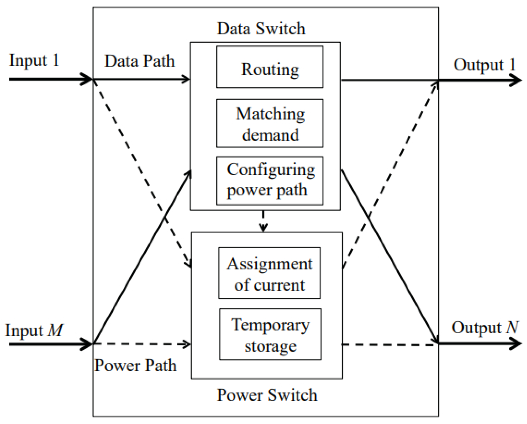Figure 1 shows the architecture of a power router. This power router comprises a power path, which delivers energy to loads, and a data path, which transmits the information to monitor the demand and supply of energy. The inputs and outputs of the power router handle data and power. Here, energy is aggregated or partitioned by the router to supply amounts that match those requested.

In this paper, we focus on operating expenses (OPEX) of the use of power routers in a DMG. We consider losses on the transmission of power to be the associated costs. We consider two sources of losses: transmission lines and power routers. The lines may have a constant loss or one proportional to the energy transmitted. We adopt the latter one. The routers have power losses inherent to the transfer of energy from one input to an output, associated with the power router operation. Also, because the microgrid may be extended, there may be a cost associated with these extensions, as worst-case scenarios. For simplicity, and without losing generality, we associate these cost-rates to each link. Because some links and paths may incur costs as power flows through them, it is of interest to minimize the cost (or overhead) of power distribution in the DMG. We also address the practical issue of how links can be interconnected to enable multiple supply paths between sources and loads, and are also useful for fault-tolerant purposes. A router with many legs may enabled us to set up a complex network that includes redundant paths in the microgrid.

Moreover, the presence of multiple DERs allows the supply to a load by a single or multiple energy sources and an energy source to supply single or multiple loads. Thus, matching loads to sources was also a process included in the routing of energy in a DMG. The minimum cost routes include the assignment of sources to loads through minimum cost paths.

2.1. Problem Definition

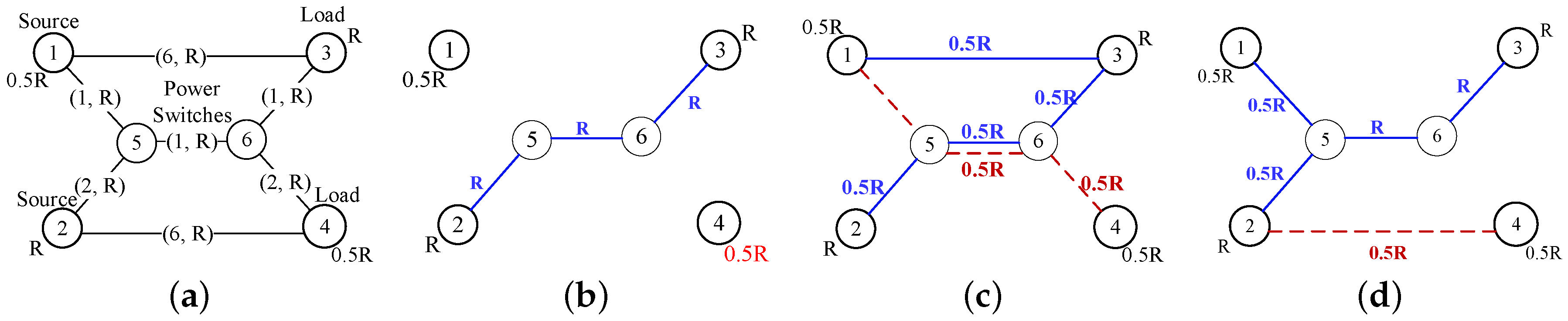
The following example depicts the path and source assignment problem in the supply of power requests in a DMG. Figure 2a shows an example of a simple DMG. This network has two sources (nodes 1 and 2), two loads (nodes 3 and 4), and two power routers (nodes 5 and 6). The two power routers provide a path with links that share the power transmitted to both loads. Each source has a supply capacity indicated by the labels (0.5R units for node 1 and R units for node 2), and the number on each link indicates the cost per unit of transmitted power and the capacity (i.e., the amount of power that the link can carry) as (p, q), respectively. Each load requests an amount of power, as indicated by the labels beside the node.

In this example, node 3 requests R units of power, and node 4 requests 0.5R units. Figure 2b shows a path for transmitting power from node 2 (source) to node 3. This path has a low cost but leaves a load request unsatisfied as there is no other path to connect to node 1 and because the shared link (link from node 5 to node 6) has reached its capacity with the flow from node 2 to node 3. The figure shows the flow that supplies power to Node 3 as a solid blue line. Figure 2c,d shows the flow that supplies node 4 as a dashed red line. Figure 2c shows that the selected paths satisfy all requests, but the total cost is high (7R). Figure 2d shows a solution where the two loads are also satisfied, and the cost is the lowest. This solution also shows an example of a source supplying two loads (node 2) and a load receiving energy from two sources (node 3).

As the example shows, the optimal routing of power in a DMG comprised of (a) the selection of the lowest-cost path to supply each load, (b) the selection of sources that supply energy according to their generation capacities, and (c) the consideration of the link transmission capacities.

2.2. Optimal Solution: Integer Linear Programming Formulation

We model the selection of paths with the smallest cost as an optimization problem to minimize the energy cost on the distribution of energy. The cost and losses in the distribution network of the DMG were linear and expressed with integer numbers, therefore, ILP is suitable for solving this optimization problem. We first modeled the DMG as a distribution network. Consider $G=(V,E)$ be a graph with two special vertices: a source s and a sink t. Here, u, where $u\in V$, is a node in the set of nodes V and edge $(i,j)$, such that $(i,j)\in E$, in the set of edges E. Every edge has a capacity $cap(i,j)\ge 0$ and a cost or weight associated with that edge. The capacity and cost are two main features of the edges in the graph that indicate the maximum capacity of the link and cost per power unit (kW) transmitted, respectively. One or multiple flows may use one edge. A flow is a real-valued function on edges that occupies a portion of the power capacity of a link, and it is indicated as $f(i,j)$. In practice, one can set the transmitted capacity as the amount of power (or current) that the link can carry and that the source can provide. The properties of a flow are as follows:

• Capacity constraints: $f(i,j)\le cap(i,j)$. If $f(i,j)=cap(i,j)$, we say that edge $(i,j)$ is saturated.
• Flow conservation (at each node except the sources and sinks): $\sum f(i,j)=0,\forall i\in V-\{s,t\}$. This property indicates that all flows that enter a transport (router) node also exit that node. Here, we assume that the switching of power has insignificant energy overhead.

The set of ILP equations describe the network model, the selection of paths and the matching between loads and sources. This set of equations consists of an objective function and a set of constraints. The objective function is defined as follows:

$$min\sum _{(i,j)\in E}{d}_{ij}{x}_{ij}.$$

(1)

Subject to:

$$0\le s_i,\forall i\in V_s$$

(2)

$$0\le t_j,\forall j\in V_t$$

(3)

$$\sum _{j:(i,j)\in E}{x}_{ij}-\sum _{j:(j,i)\in E}{x}_{ji}=s_i,\forall i\in V_s$$

(4)

$$\sum _{i:(i,j)\in E}{x}_{ij}-\sum _{i:(j,i)\in E}{x}_{ji}=t_j,\forall j\in V_t$$

(5)

$$\sum _{j:(i,j)\in E}{x}_{ij}-\sum _{j:(j,i)\in E}{x}_{ji}=0,\forall i\in V-V_s-V_t$$

(6)

$$0\le x_{ij}\le cap(i,j),\forall (i,j)\in E,$$

(7)

where $x_{ij}$ is the amount of power the generator transmits to the load, $d_{ij}$ is the cost per unit of power edge $(i,j)$ carries, $s_i$ and $t_j$ are the amount of power source i generates and sink j requests, respectively. $V_s$ is a subset of V that contains all the source nodes. Similarly, $V_t$ contains all the sink nodes. Here, (1) defines the cost minimization function, (2) and (3) are constraints corresponding to the amount of power generated by the sources and required by the sinks, (4) and (5) describe the conservation of energy flow of the power sources and sinks, respectively, (6) describes the conservation of energy flow of the transport nodes, and (7) shows the capacity constraint for each link. The complexity of the optimal method for the selection of the smallest cost path is $O(n^{\left(2\right|V|+2)}{\left(\right|V\left|a\right)}^{\left(\right|V|+1)\left(\right|V|+2)})$ where n is the largest number of legs of a network node, $a=max\left\{\right|(i,j)|,|V_s|,|V_t\left|\right\}$; the largest link cost, source capacity, and load demand, and $\left|V\right|$ is the number of nodes in the network.

2.3. Greedy Smallest-Cost-Rate Path First (GRASP) Algorithm

Although the optimal method converges to an optimal solution for energy allocation in the presence of multiple energy sources and loads, the method is NP-hard, so that its complexity is prohibitively high for a network with a considerable number of nodes [31]. GRASP aims to match sources and loads and, in combination, find the smallest cost-rate paths in between, restricted to the source and link capacities, and the losses associated to links. By using the cost rates, GRASP aims to obtain a small routing cost. It should be noted that this smallest cost rate may not be the smallest overall cost but the use of this parameter reduces the complexity of finding the paths in comparison with the optimal method. The algorithm operates in an iterative and greedy approach, and its objective is also described by the objective function and constraints in Section 2.2. GRASP finds the k shortest cost-rate paths, one per each load-source pair and matches loads (demands) to as many sources as needed with an aggregate capacity generation that is able to satisfy the power demands of the loads.

There are other constraints in this problem: (a) the amount of power that the selected path can carry was set by either (1) the link with the smallest of power capacity; (2) the capacity of the power source and; (3) the amount of power the customer requests. (b) The selection of a path cannot select a congested link (i.e., a link carrying an amount of power equal to its capacity) for accommodating another request. Because different sources may partially fulfil the power requested by a load, the number of paths needed to supply a demanding load may be many. A routing algorithm must select the sources needed to satisfy a load demand and whose path to the source(s) incurs in the minimum transmission costs. This property is a significant difference between routing in a DMG and that in computer networks.

GRASP works as follows:

Step 1.

Find all smallest cost-rates paths between for all load and sources.

Step 2.

Select the path with the smallest cost rates among those in step 1, while considering the amount of power (generation) capacity of the source, the link capacities, and the amounts of power requested by the loads.

Step 3.

Reserve the portion of the path and source capacity for the routed flow and consider that portion of the request satisfied (if not all).

Step 4.

Decrease the capacity of each link on the selected path and source by the minimum of the requested amount and that granted. If the portion of available power left on one of the links of the selected path or sources reaches zero, delete this link or source from the set obtained in step 1.

Step 5.

Increase the amount of power granted to the load, and if the request is full satisfy it, consider this load satisfied.

Step 6.

Repeat the process, starting from step 1, until all the customers receive all the requested power or not paths or source remains available for supplying the requested amount of power.

The pseudocode of this algorithm, presented in Algorithm 1, shows a greater level of detail.

Therefore, it is easy to see that the complexity of GRASP is the complexity of the smallest-cost-rate link search or $O\left(\right|E\left|log\right|V\left|\right)$ [32] times the number of loads times the number of sources, or $O\left(N_s{N}_L\right|E\left|log\right|V\left|\right)$, where $N_s$ is the number DERs, $N_L$ is the number of loads whose power requests are satisfied, and $\left|E\right|$ is the number of links in the network.

Algorithm 1 Greedy smallest-cost-rate path first (GRASP).

1: procedure calculate Total Cost 2:     Initialize a connected graph $G(V,E)$ 3:     $\mathit{total}\_\mathit{cost}\leftarrow 0$ 4:     path ← smallest-cost-rate paths for source-load pairs 5:     $\mathit{cost}\leftarrow \mathrm{costs}\mathrm{of}\mathrm{path}\left(\mathrm{i}\right)\mathrm{in}\mathit{path}$ 6:     loop: 7:     if $\mathrm{not}\mathit{path}\mathrm{and}\mathrm{one}\mathrm{or}\mathrm{more}\mathrm{loads}\mathrm{request}\mathrm{power}$ then 8:         return $Nopaths;End$ 9:     if $\mathrm{no}\mathrm{load}\mathrm{request}\mathrm{power}$ then 10:         return $\mathit{total}\_\mathit{cost}$ 11:     else 12:         $\mathit{min}\_\mathit{cost}\leftarrow \min \left(\mathit{cost}\right)$ % here cost is the cost rate 13:         $\mathit{p}\leftarrow \mathrm{the}i-\mathrm{th}\mathrm{path}\mathrm{with}\mathit{cost}\left(i\right)==\mathit{min}\_\mathit{cost}$ 14:         $\mathit{cap}\_\mathit{s}\leftarrow \mathrm{power}\mathrm{capacity}\mathrm{of}\mathrm{source}\mathrm{on}\mathrm{path}p$ 15:         $\mathit{req}\_\mathit{l}\leftarrow \mathrm{power}\mathrm{demands}\mathrm{of}\mathrm{load}\mathrm{on}\mathrm{path}p$ 16:         $\mathit{link}\_\mathit{p}\leftarrow \mathrm{capacity}\mathrm{of}\mathrm{all}\mathrm{the}\mathrm{links}\mathrm{on}\mathrm{path}p$ 17:         $\mathit{min}\_\mathit{link}\_\mathit{p}\leftarrow \mathrm{minimum}\mathrm{path}\mathrm{capacity}p$ 18:         $\mathit{min}\_\mathit{tran}\leftarrow \min (\mathit{cap}\_s,\mathit{req}\_l,\mathit{min}\_\mathit{link}\_p)$ 19:         $\mathit{total}\_\mathit{cost}\leftarrow \mathit{total}\_\mathit{cost}+\mathit{min}\_\mathit{tran}*\mathit{cost}\left(\mathit{i}\right)$ 20:         $\mathit{cap}\_\mathit{s}\leftarrow \mathit{cap}\_\mathit{s}-\mathit{min}\_\mathit{tran}$ 21:         $\mathit{req}\_\mathit{l}\leftarrow \mathrm{req}\_\mathrm{l}-\min \_\mathrm{tran}$ 22:         $\mathit{link}\_\mathit{p}\left(\mathit{i}\right)\leftarrow \mathit{link}\_\mathit{p}\left(\mathit{i}\right)-\mathit{min}\_\mathit{tran}\forall \mathrm{links}\mathrm{of}\mathrm{path}p$ 23:         $\mathbf{update}\mathit{path}\mathbf{and}\mathit{cost}:$ 24:         $\mathit{s}\leftarrow \mathrm{source}\mathrm{of}\mathrm{path}p$ 25:         $\mathit{l}\leftarrow \mathrm{load}\mathrm{of}\mathrm{path}p$ 26:         $\mathit{link}\_\mathit{min}\leftarrow \mathrm{link}\mathrm{with}\min \mathrm{capacity}\mathrm{of}\mathrm{path}p$ 27:         if $\mathit{min}\_\mathit{tran}==\mathit{cap}\_\mathit{s}$ then 28:            $\mathrm{delete}\mathrm{all}\mathrm{the}\mathrm{paths}\mathrm{including}\mathrm{source}s$ 29:            $\mathrm{delete}\mathrm{the}\mathrm{costs}\mathrm{from}\mathit{cost}$ 30:         if $\mathit{min}\_\mathit{tran}==\mathit{req}\_\mathit{l}$ then 31:            $\mathrm{delete}\mathrm{all}\mathrm{the}\mathrm{paths}\mathrm{connected}\mathrm{to}\mathrm{load}l$ 32:            $\mathrm{delete}\mathrm{the}\mathrm{costs}\mathrm{of}\mathit{cost}$ 33:         if $min\_tran==min\_link\_p$ then 34:            if $\mathit{link}\_\mathit{min}\mathrm{in}\mathrm{graph}\mathit{G}$ then 35:                    $\mathrm{delete}\mathit{link}\_\mathit{min}$ 36:            $\mathrm{find}p\_\mathit{new}\mathrm{with}\mathrm{the}\mathrm{smallest}-\mathrm{cost}\mathrm{rate}\mathit{cost}\_\mathit{new}$ 37:            $\mathrm{add}p\_\mathit{new}\mathrm{and}\mathit{cost}\_\mathit{new}\mathrm{to}\mathit{path}\mathrm{and}\mathit{cost}$ 38:         goto loop

3. Results and Analysis

Here, we evaluate the total cost incurred by the optimal method and GRASP. We show the application of both methods on two different networks. One was a simple network and the other was National Science Foundation (NSFNET). While NSFNET was not a power network, was is an example of a network with a different number of paths between two nodes (as in computer networks). It also shows how a power distribution bus may look after the adoption of power routers. We also consider different IEEE test buses, which found their use in various power tests. Some of these networks had a small number of power sources and loads, and others had a large number of both, thus presenting different scenarios. These networks offered different examples of the application of multi-leg nodes and a variety of paths.

3.1. Example DMG Networks

3.1.1. A Simple Network

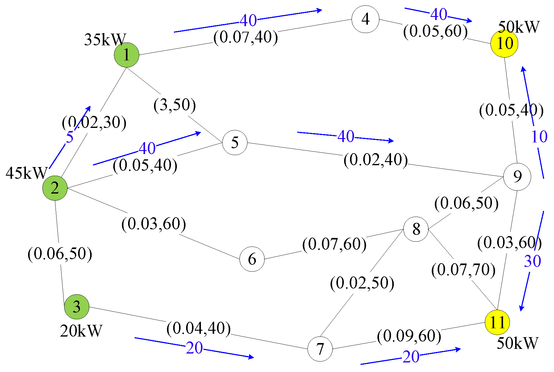
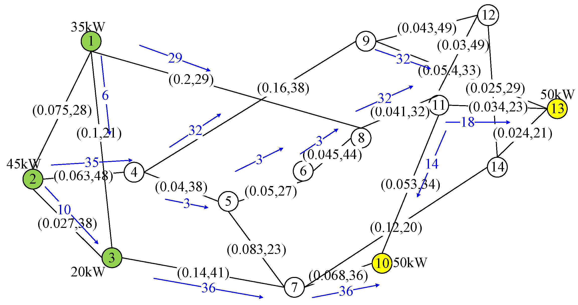
First, we consider a simple network, as Figure 3 and Figure 4 show. These figures show the cost and capacity link assignment and source capacity for case 1. In the remainder of this paper, we show diagrams for case 1 of the considered networks. In this network, there are three power sources, nodes 1–3, depicted in green color. Each source node had a generation capacity of 35 kW, 45 kW, and 20 kW, respectively, resulting in a total generation of 100 kW available to the two loads; nodes 10 and 11, depicted in yellow color. Each load requested 50 kW. We indicate both the cost (e.g., power loss) per unit of power transmitted through it and power capacity of each link on the network.

We consider three test cases per network. We assigned an arbitrary cost and capacity per link in case 1. We modified the costs and link capacity of the links in case 2 to test the selection of a different path. We changed the amount of power capacity of sources and demand (requests) for driving the loads to match with different sources, leading to a varied selection of paths, in case 3.

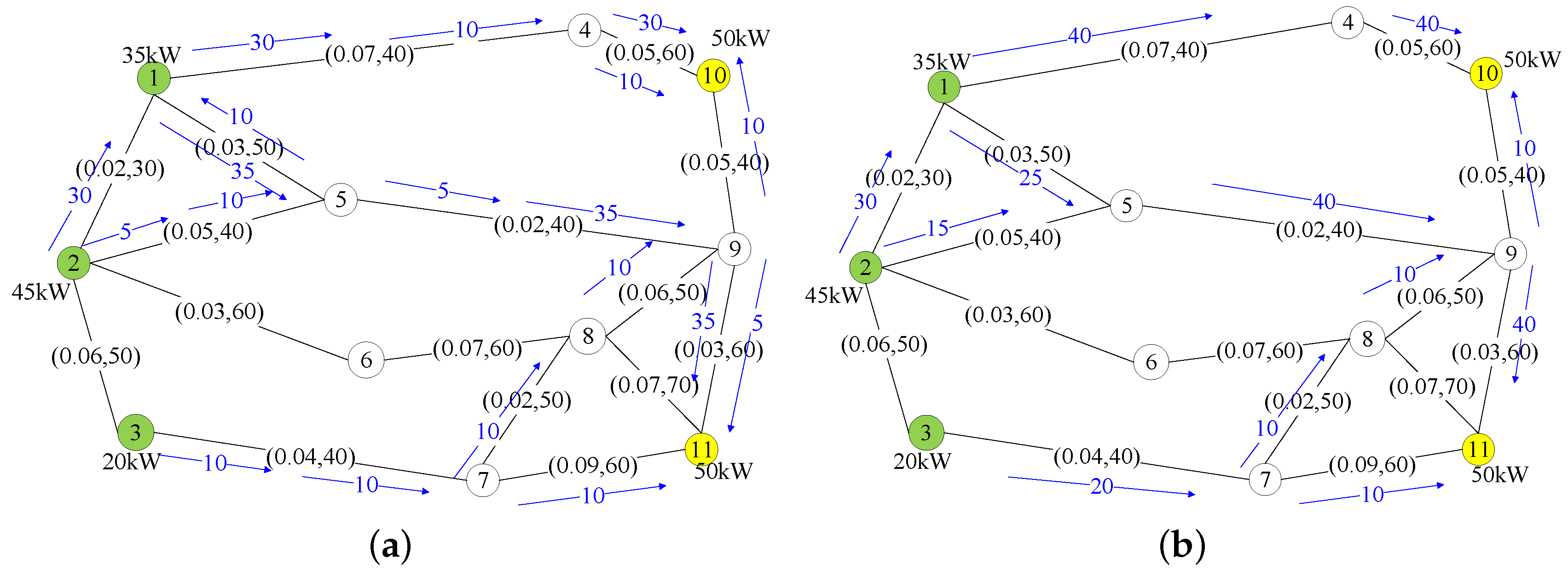
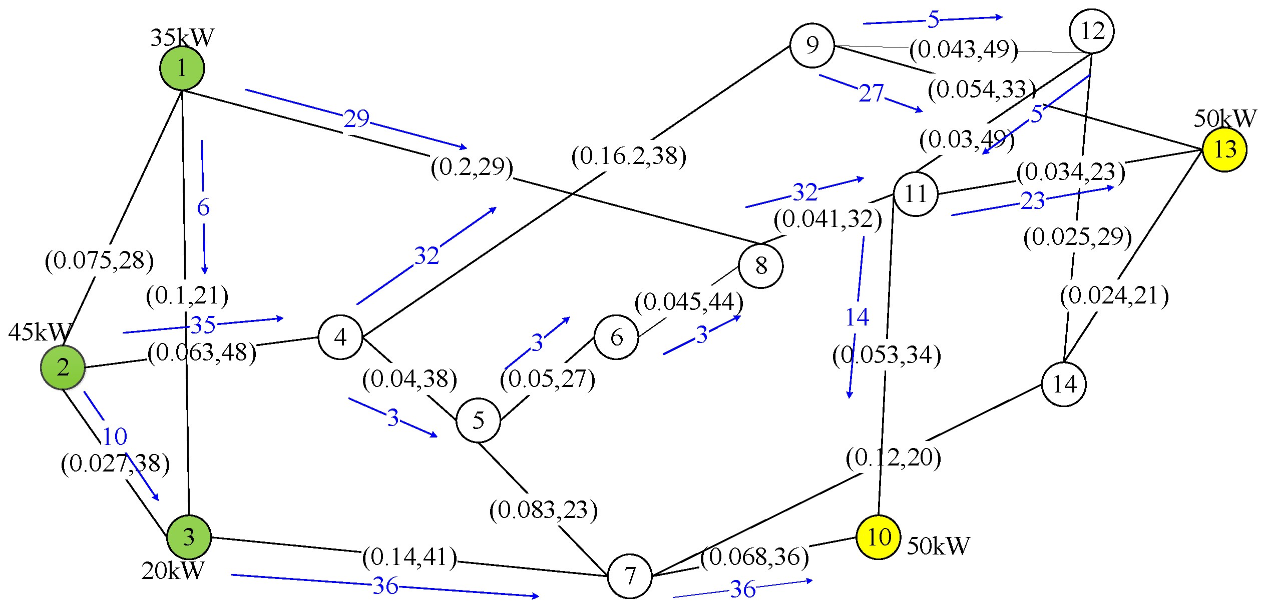
In general, the GRASP algorithm greedily selects the smallest-cost-rate path of all the source-load pairs in each iteration. As shown in line 4 of the pseudocode, the smallest-cost-rate paths of all source-load pairs are pre-calculated and cached in a list path. For each iteration of the loop, in line 13, path p, which is the smallest one amount the paths in path, will be selected and the source of this path is assigned to the load of this path. To show how the proposed GRASP algorithm works, we took the simple network as an example. As shown in Figure 4a, the blue arrows show the selected paths by using GRASP. First, GRASP calculates the smallest-cost-rate path of all the source-load pairs. It selects the path $1\to 5\to 9\to 11$, where $a\to b$ means a link selected from node a to node b, that has a cost rate equal to 0.08. Then source 1 transmits 35 kW of power through as limited by its capacity. Then, it selects $2\to 5\to 9\to 11$ as the second smallest-cost-rate path, to transmit 5 kW because this is the maximum power that could be transmitted form node 5 to 9 as 35 kW were already reserved on this link. GRASP keeps going in this way until all the power demands are satisfied.

A path from a source to a load can be represented by the path cost, which is the sum of link costs, and the path capacity, which is the capacity of the link with the smallest power capacity of all links comprising the path. The total cost is the sum of incurred flow costs on each link:

$$C_t=\sum _{(i,j)\in E}{d}_{ij}{x}_{ij},$$

(8)

where $C_t$ is the total cost, $d_{ij}$ is the cost per unit of power transmitted on edge $(i,j)$, and $x_{ij}$ is the amount of power transmitted on edge $(i,j)$.

Figure 3 and Figure 4 also show the selected paths and the amounts of power granted over each selected path, as blue arrows, selected by the optimal method and GRASP, respectively. As Figure 4a shows, some power flows share some of the links in the selected paths as they are associated with small costs. Figure 4b shows the total power flowing on each link. 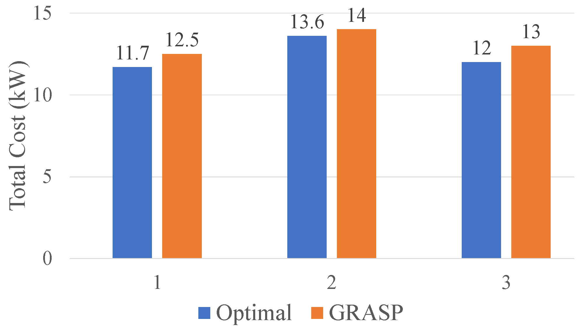The power on the links is the sum of the individual power per flow shown in Figure 4. We use this representation of results in the remainder of this paper. In the network, the total cost of routing power from all the sources to all the loads was 12.7 kW. However, the total cost achieved by GRASP was 13.5 kW or an increase of 6.3% over the optimal solution. We also performed a test for cases 2 and 3 (we do not show the figures for these two cases because of the limited space). In case 3, the power capacity of nodes 1–3 were 40 kW, 40 kW, and 20 kW, respectively, and the amount of power requested by nodes 10 and 11 was 70 kW and 30 kW, respectively. 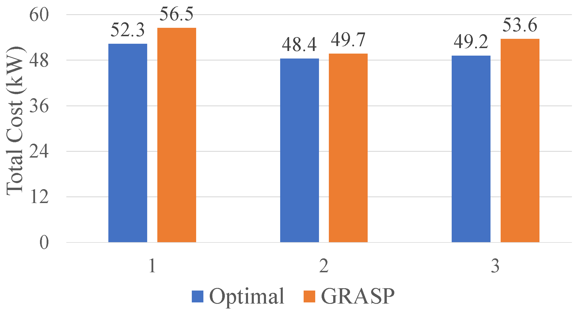Figure 5 shows the comparisons of the total cost incurred by the optimal method and GRASP for each the three cases. As the figure shows, GRASP achieved a cost of 8.33% above the optimal costs as the worst case of the tested scenarios.

We also performed route calculations on more complex networks, such as NSFNET [33], IEEE14 test [34] and IEEE39 test buses [35,36]. In this section, we present the total cost recurred by GRASP and the optimal method. Similarly, as in the simple network discussed above, we consider three different cases for each network.

3.1.2. NSFNET

This network is the result of a program of coordinated and evolving projects sponsored by the National Science Foundation (NSF) that was initiated in 1985 to support and promote advanced networking among U.S. research and education institutions. Figure 6 and Figure 7 show this network. This network had three sources and two loads, as in the simple network, but it also had a larger number of links and a higher node degree. The increased number of links in this network enabled a wider selection of independent paths (i.e., paths with fewer or no shared link) of source-load pairs. Particularly to this network, the cost of each link is directly proportional to the geographical distance between two nodes (each node in NSFNET is a U.S. city) and the capacity of each link was set arbitrarily.

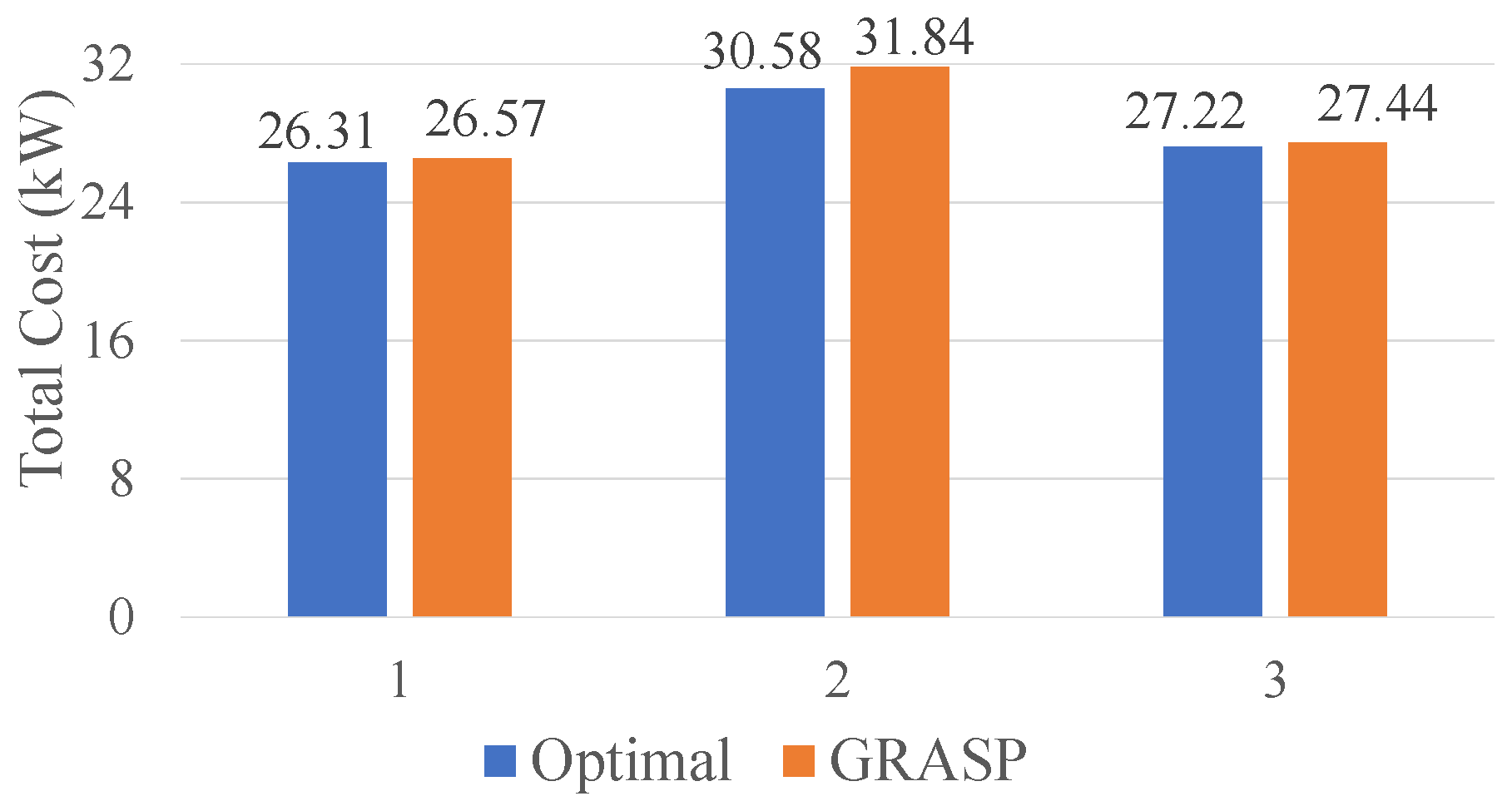
Figure 6 and Figure 7 show the results of case 1 in NSFNET as resolved by the optimal method and GRASP, respectively. Figure 8 shows the overall cost results obtained by these two methods. These results indicate that GRASP fell 3.9% short of achieving the optimal solution by an increase of about 12.6 kW in case 2. Similarly to the simple network, case 2 of the NSFNET network used different link costs and link power capacities from case 1, while case 3 used different power source capacities and demands of power. Case 2 then is used to observe different route selection from case 1 as link costs are modified, and case 3 may lead to the use of different paths but triggered by a different distribution on power generation and demand. From these two cases, case 2 draws the larger discrepancy between these two methods. However, the differences between the optimal solution and GRASP in the NSFNET network are smaller than those achieved in the simple network. A possible cause of this improvement is the larger number of routing options provided by the larger number of links and node order in NSFNET.

Considering the complexity of NSFNET, the matching of sources and loads and the selected distribution paths in this network is also represented by a power routing table, as

Table 1. Power assigned to the links of the NSFNET network by using the optimal method.

Energy Routing Table (kW)
Node	1	2	3	4	5	6	7	8	9	10	11	12	13
1	0	0	6	0	0	0	0	29	0	0	0	0	0
2	0	0	10	35	0	0	0	0	0	0	0	0	0
3	-6	−10	0	0	0	0	36	0	0	0	0	0	0
4	0	−35	0	0	3	0	0	0	32	0	0	0	0
5	0	0	0	−3	0	3	0	0	0	0	0	0	0
6	0	0	0	0	−3	0	0	3	0	0	0	0	0
7	0	0	−36	0	0	0	0	0	0	36	0	0	0
8	−29	0	0	0	0	−3	0	0	0	0	32	0	0
9	0	0	0	−32	0	0	0	0	0	0	0	0	32
10	0	0	0	0	0	0	−36	0	0	0	−14	0	0
11	0	0	0	0	0	0	0	−32	0	14	0	0	18
12	0	0	0	0	0	0	0	0	0	0	0	0	0
13	0	0	0	0	0	0	0	0	−32	0	−18	0	0

and

Table 2. Power assigned to the links of the NSFNET network by GRASP.

Energy Routing Table (kW)
Node	1	2	3	4	5	6	7	8	9	10	11	12	13
1	0	0	6	0	0	0	0	29	0	0	0	0	0
2	0	0	10	35	0	0	0	0	0	0	0	0	0
3	−6	−10	0	0	0	0	36	0	0	0	0	0	0
4	0	−35	0	0	3	0	0	0	32	0	0	0	0
5	0	0	0	−3	0	3	0	0	0	0	0	0	0
6	0	0	0	0	−3	0	0	3	0	0	0	0	0
7	0	0	−36	0	0	0	0	0	0	36	0	0	0
8	−29	0	0	0	0	−3	0	0	0	0	32	0	0
9	0	0	0	−32	0	0	0	0	0	0	0	5	27
10	0	0	0	0	0	0	−36	0	0	0	−14	0	0
11	0	0	0	0	0	0	0	−32	0	14	0	−5	23
12	0	0	0	0	0	0	0	0	−5	0	5	0	0
13	0	0	0	0	0	0	0	0	−27	0	−23	0	0

. These tables correspond to the path selection presented in Figure 6 and Figure 7, as obtained by the optimal method and GRASP, respectively. These tables show the amounts of power assigned to the different links. In each table, $x_{ij}$ means the amount of power transmitted from node i to node j. A positive $x_{ij}$ means that the power flows from node i to node j and a negative $x_{ij}$ means that the power flows from node j to node i (opposite direction). Also, if $x_{ij}=0$, there is no power flow between nodes i and j.

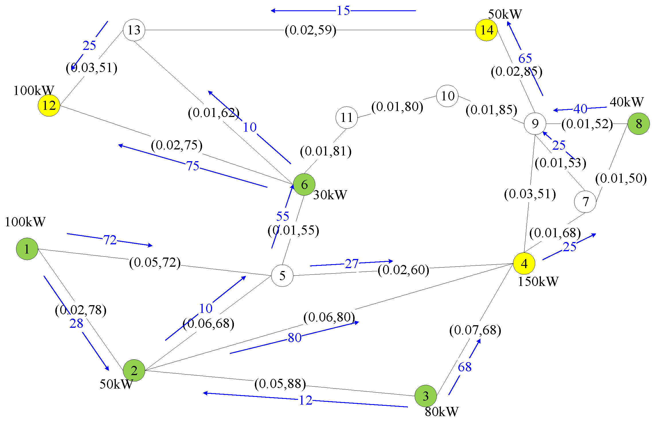
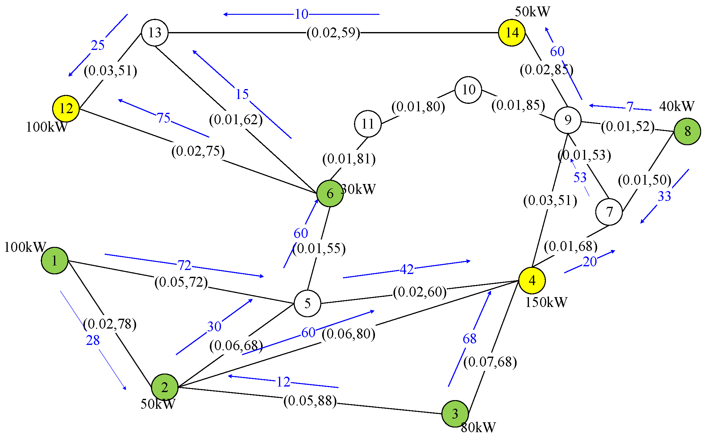
3.1.3. IEEE14 Bus

The IEEE14 bus system [34] represents a simple approximation of the American Electric Power system as of February 1962. This test bus has 14 buses, five generators (i.e., sources), and 11 loads.

However, to stress the performance of GRASP in this network, we assume only three loads from those in the bus. In this way, we increase the search space to match the loads to the sources as the number of sources is much larger than the number of loads. Figure 9 and Figure 10 show the matched pairs and resulting paths by the two considered schemes. The data in the figures indicate the amount of power provided by the sources and requested by the loads and the cost and capacity of each link of case 1.

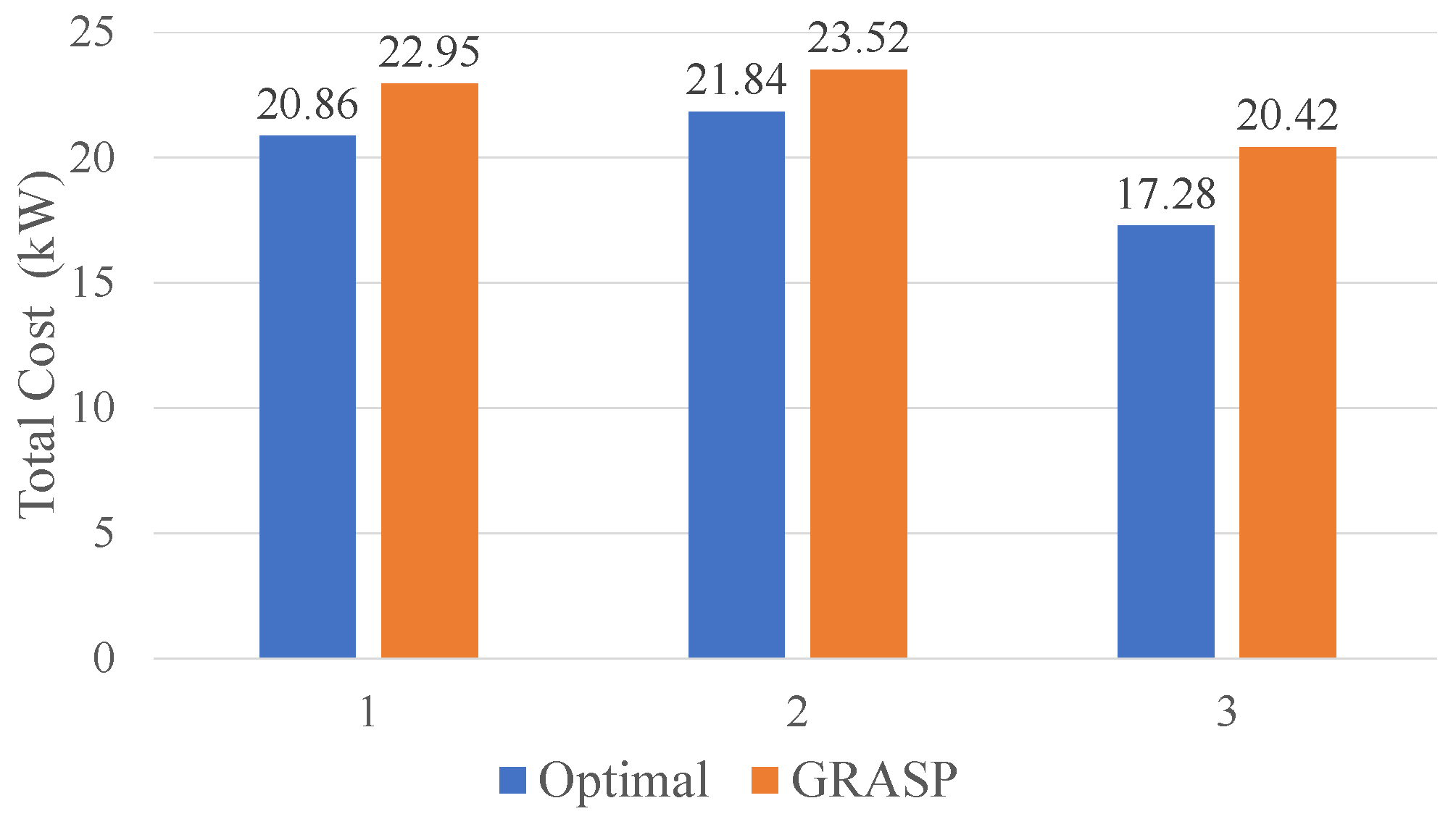
The results in this figures show that the total cost of the paths selected by GRASP is comparable to that achieved by the optimal method, as Figure 11 shows. The largest discrepancy in this scenario was 18.0%, which was the additional cost incurred by the selections GRASP make.

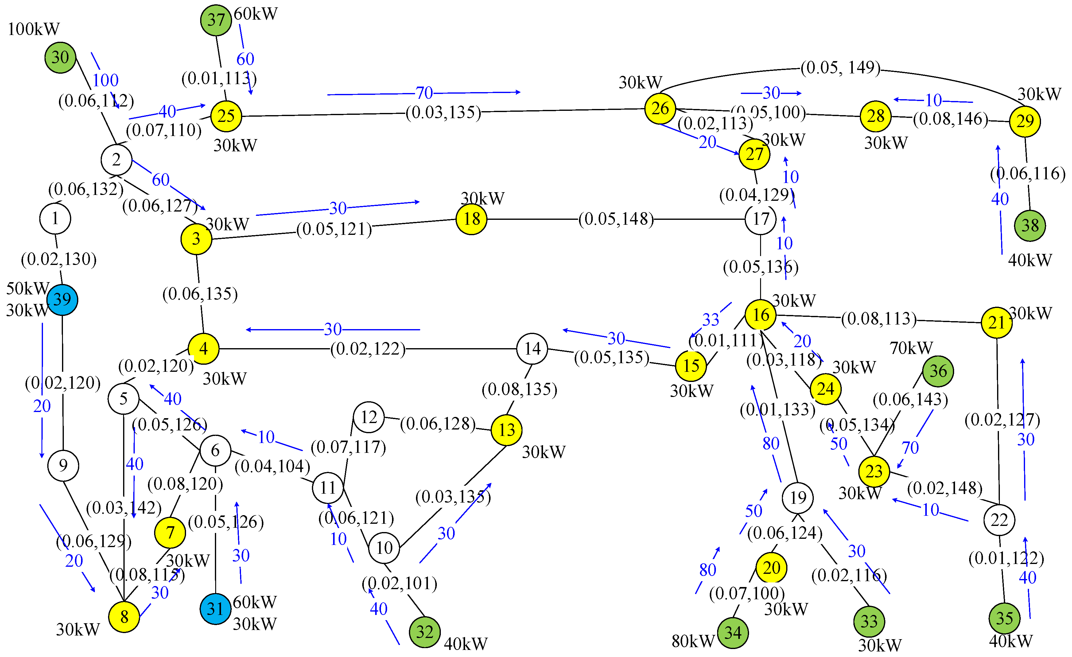
3.1.4. IEEE39 Bus

This was a large bus, it had 39 buses, 46 transmission lines, 10 power sources, and 19 loads. This network had two nodes, nodes 31 and 39, represented in blue color, that performed a combined functional mode; each node generated and spent energy. These two nodes played both roles; a power source and a load, at the same time.

Figure 12 and Figure 13 show the results obtained by the optimal method and GRASP on this test bus. With the larger number of sources and customers, the IEEE39 test bus showed a much more complex scenario than the three previous network topologies. Here, loads had a larger number of choices of sources to select, but the number of links and node order is equal to or smaller than those considered in NSFNET. It was expected that there were fewer choices for routing power in this test bus than in NSFNET and at the same time, more flows needed to be routed by the larger number of loads in this test bus.

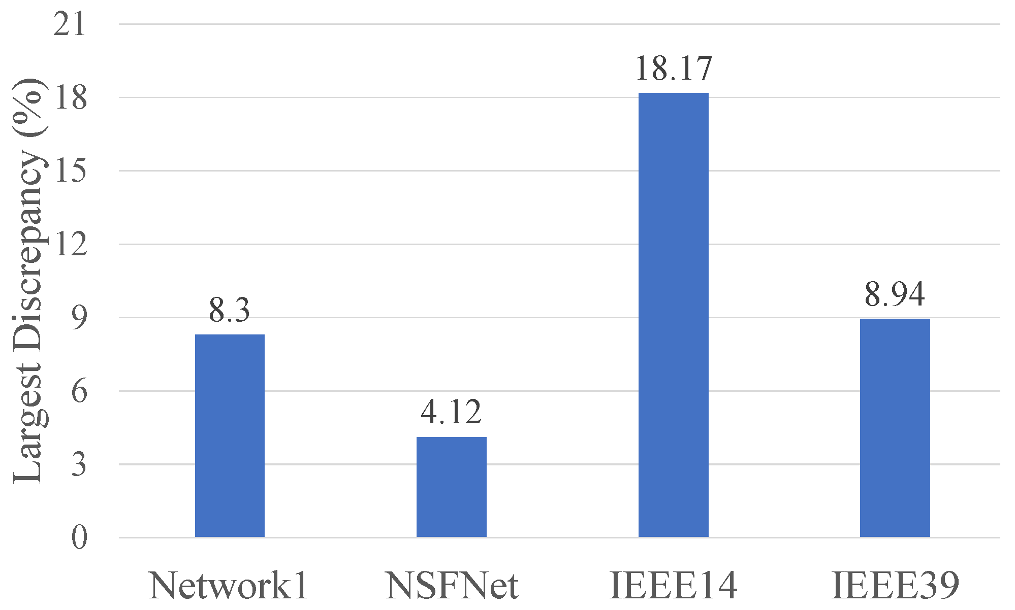
Figure 14 shows a comparison of the different cases tested on this network. This graph shows that GRASP achieves 9% as the most substantial additional cost in comparison to the optimal solution in case 3. Figure 15 shows the largest additional cost incurred by GRASP in comparison to those obtained by the optimal method for the three considered networks and cases.

3.2. An Example of a Practical Application of GRASP

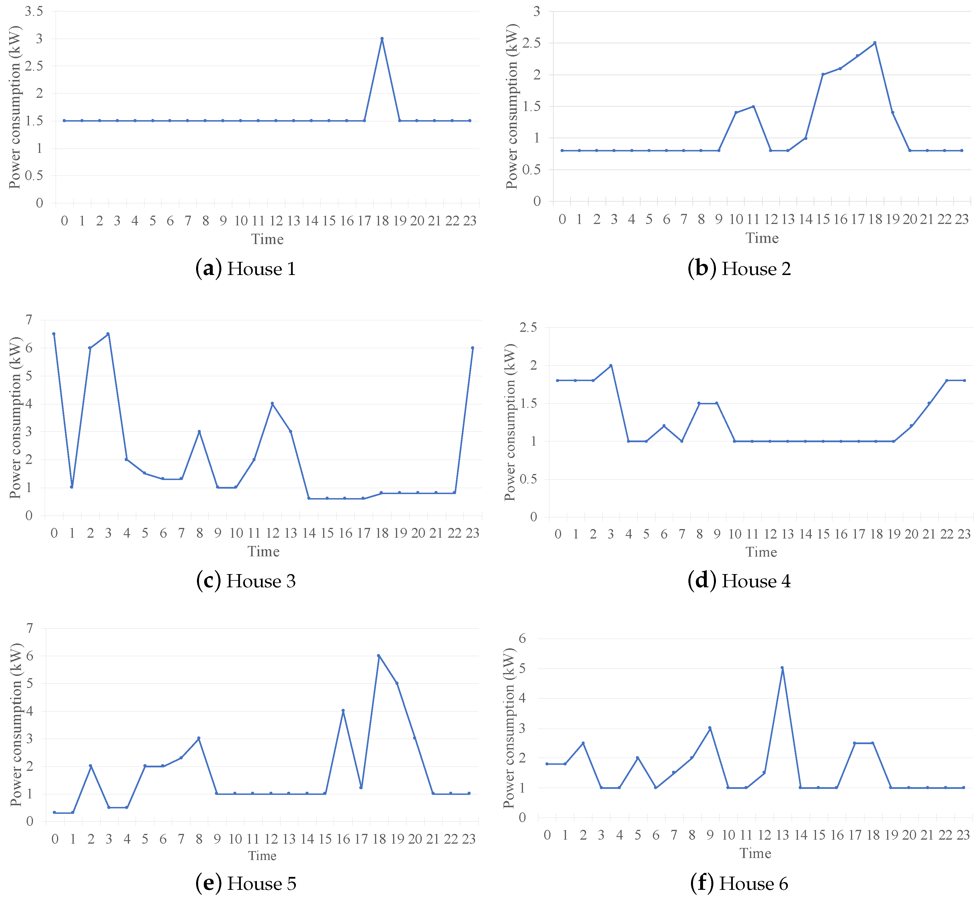
We used low-frequency power data collected from six houses from the Reference Energy Disaggregation Data Set (REDD) [37]. The data of each house consisted of power consumption information measured from different appliances, such as a refrigerator, lighting, microwave, etc. The data contained power consumption from real homes, for the whole house as well as for each circuit in the house (labeled by the main type of appliance on that circuit).

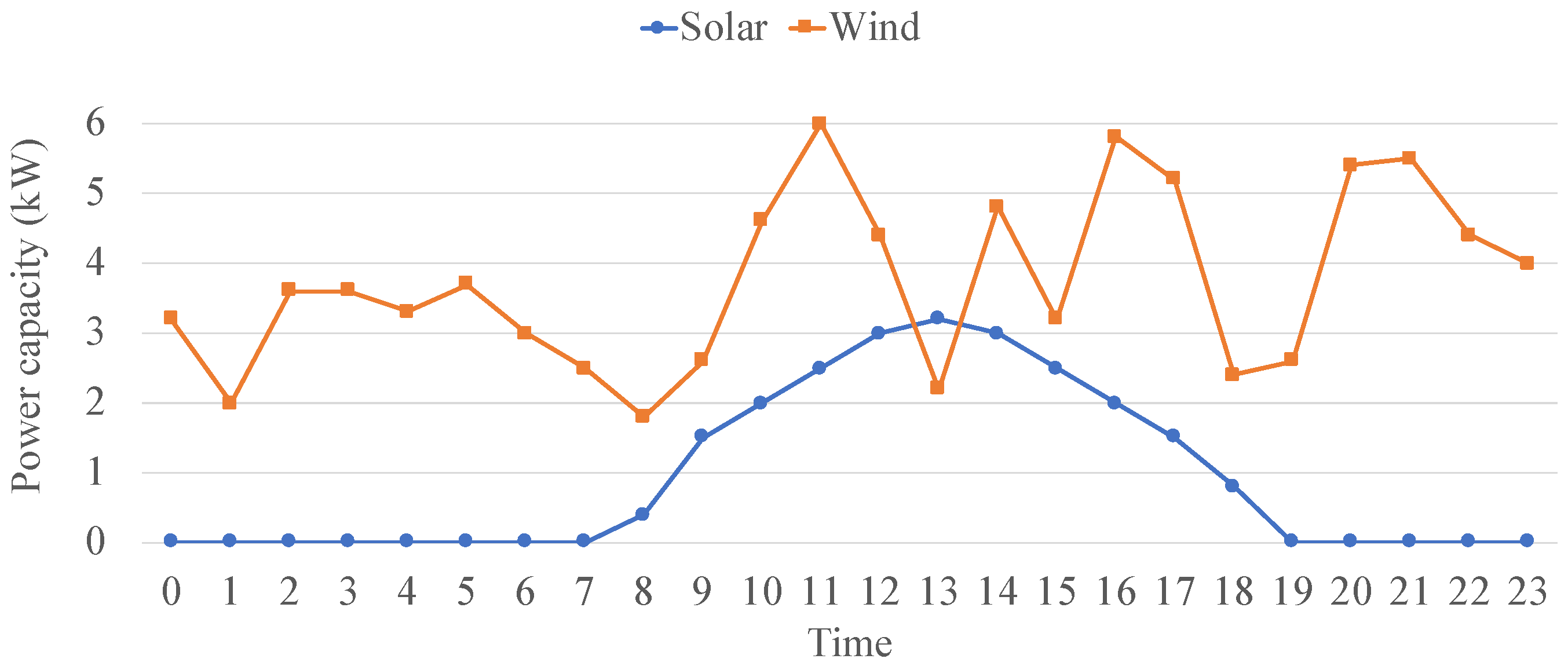
We used the power consumption profile of six different houses as loads and five different energy sources. Figure 16 shows the power profiles for 24 h of the six loads. The energy resources were three photovoltaic (solar) generators [38] and two wind turbine generators [39]. We used the same power profile for the solar and wind sources. Figure 17 shows the profile of the solar and wind generators.

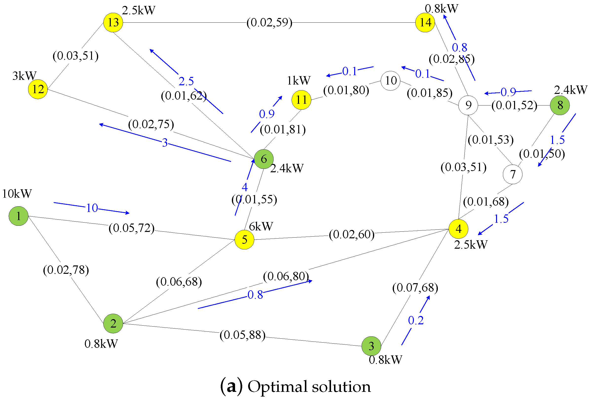
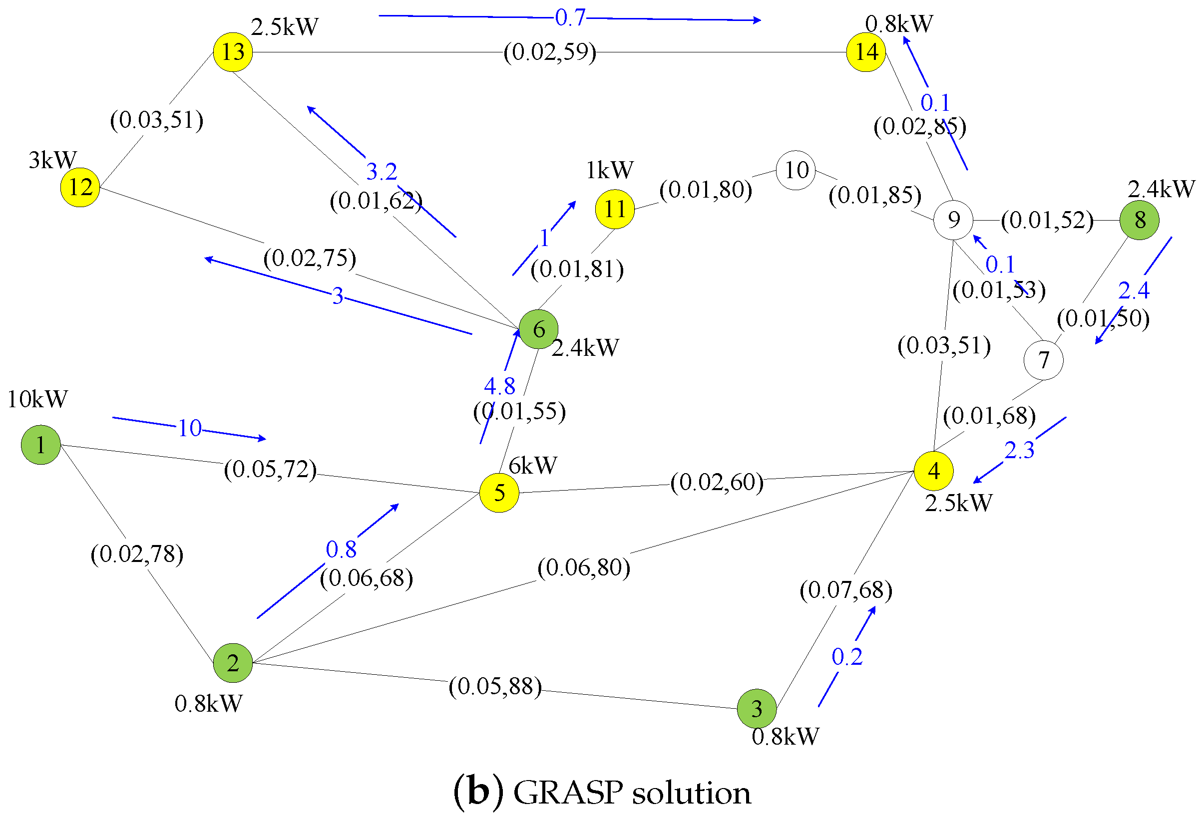
We used the IEEE 14 testbus to interconnect the sources and loads. In this practical example, we used one generator of constant power (power line) as node 1, two identical Solar generators as nodes 2 and 3, and two identical wind-turbine generators, as nodes 6 and 8. The power capacity of the constant power generator is 10 kW. The loads in this testbus were Nodes 12, 13, 14, 11, 5, and 4 as houses 1–6, respectively.

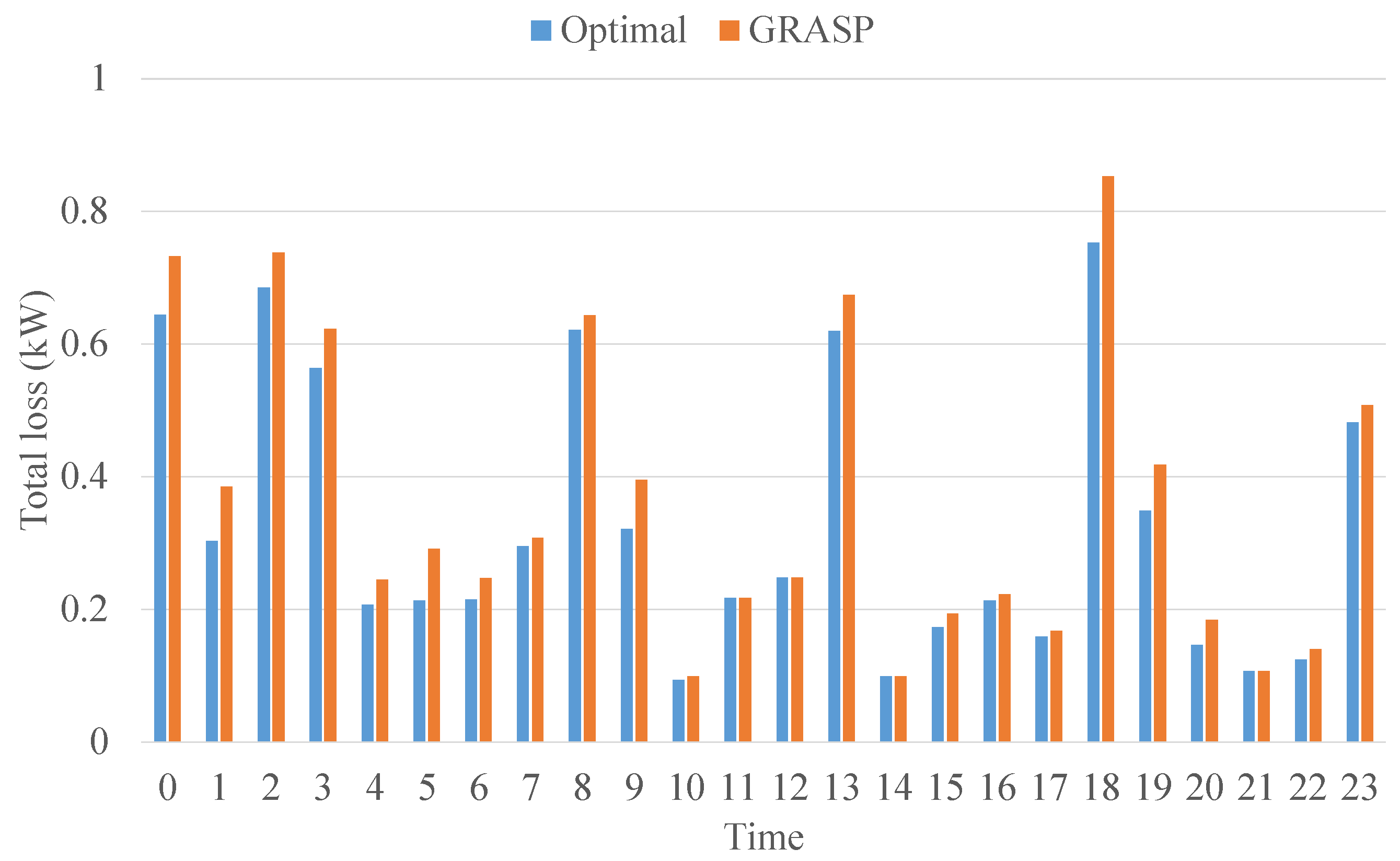
We performed power routing for this example, and the summary of per-hour distribution provides the results Figure 18 shows. These results show that the largest cost discrepancy is 0.1 kW at 6 p.m. Figure 19 shows the routing of power at 6 p.m. for the optimal method and GRASP.

4. Conclusions

In a source-dense digital microgrid, the distribution of power consists of matching loads to the power sources that can satisfy their power request, and of the selection of the lowest-cost paths interconnecting them. Such paths transfer the requested amounts of power but with minimum total costs. We considered the costs incurred by a function of the power transferred through the link. To realize power routing, we first modelled the problem as an integer linear programming approach. While this method provides an optimal solution, its complexity is NP-hard. Therefore, the application of this optimal method on a digital microgrid with a large number of sources is prohibitive. As a solution, we have proposed the greedy smallest-cost-rate path first algorithm, or GRASP in short, to assign sources to loads and obtain the smallest cost routes between sources and loads. We tested GRASP on four different network topologies, including IEEE test buses. We compared the total cost obtained by the optimal method and GRASP. The results show that GRASP achieves comparable costs as does the optimal solution, with a discrepancy of up to 18% on the considered scenarios. We also present a practical application of GRASP where we use the power consumption profile of six houses and the actual power generation profile of five sources on IEEE14 testbus and show the differences between the optimal method and GRASP. We showed that the largest discrepancy cost in this example is 0.1 kW. Our analysis also shows that GRASP achieves these additional costs in exchange for a computation complexity smaller than that of the optimal method.