Article

An Improved Signal Processing Approach Based on Analysis Mode Decomposition and Empirical Mode Decomposition

1
The School of Mechanical and Electrical Engineering, University of Electronic and Science Technology of China, Chengdu 611731, China
2
Department of Computer Science, University of North Carolina, Chapel Hill, NC 27516, USA
*
Author to whom correspondence should be addressed.
Energies 2019, 12(16), 3077; https://doi.org/10.3390/en12163077
Submission received: 25 June 2019 / Revised: 31 July 2019 / Accepted: 5 August 2019 / Published: 9 August 2019

Abstract

:
Empirical mode decomposition (EMD) is a widely used adaptive signal processing method, which has shown some shortcomings in engineering practice, such as sifting stop criteria of intrinsic mode function (IMF), mode mixing and end effect. In this paper, an improved sifting stop criterion based on the valid data segment is proposed, and is compared with the traditional one. Results show that the new sifting stop criterion avoids the influence of end effects and improves the correctness of the EMD. In addition, a novel AEMD method combining the analysis mode decomposition (AMD) and EMD is developed to solve the mode-mixing problem, in which EMD is firstly applied to dispose the original signal, and then AMD is used to decompose these mixed modes. Then, these decomposed modes are reconstituted according to a certain principle. These reconstituted components showed mode mixing phenomena alleviated. Model comparison was conducted between the proposed method with the ensemble empirical mode decomposition (EEMD), which is the mainstream method improved based on EMD. Results indicated that the AEMD and EEMD can effectively restrain the mode mixing, but the AEMD has a shorter execution time than that of EEMD.

Graphical Abstract

1. Introduction

The analysis of time-frequency of vibration signals is one of the most effective and important methods for fault diagnosis of rotating machinery, since the vibration signal includes massive information that reflects the running state of rotating machinery [1]. The empirical mode decomposition (EMD) is one of most commonly used methods for signal processing in the time-frequency domain. EMD can decompose a complex signal into the finite intrinsic mode functions (IMF) based on the local characteristic time scale of signals, and each IMF represents one intrinsic vibration mode of the original signal. Then the characteristic information of the signal can be extracted by analyzing such stationary stable IMFs [2]. EMD has attracted increasing attention since it appeared [3,4,5], and it has been widely used in economics, biomedicine and engineering science fields, especially for fault diagnosis. Ali et al. [6] applied the EMD method and artificial neural network in fault diagnosis of rolling bearings automatically. Xue et al. [7] presented an adaptive, fast EMD method and applied it to rolling bearings fault diagnosis. Yu et al. [8] introduced various applications of EMD in fault diagnosis. Cheng et al. [9] combined EMD with a Hilbert transform to conduct the recognition for mode parameters. Then, they introduced how to apply the EMD to the fault diagnosis for local rub-impact of rotors [10]. Rilling [11] investigates how the EMD behaves under the case of a composite two-tone signal.
Though EMD has been commonly utilized in reality, some shortcomings are exposed, including mode mixing, end effects, stop criteria of IMF, over-envelope and under-envelope. These deficiencies normally restrict the further promotion and application of EMD [12]. Since the criterion to judge IMF is that the average value of its upper and lower envelope spectrums is zero in the EMD method, but in the real decomposition process, that average value is impossible to be zero due to the disturbance of cubic spline interpolation, the influence of end effect and adopted frequency. Thus, it is necessary to define a valid stop criterion for the decomposition process in engineering, namely the stop criterion problem of IMF for the EMD method, also named as the sifting stop criterion. Some researchers have attempted to improve the efficiency of EMD. Among them, Pustelnik [13] mainly developed an alternative to the sifting process for EMD, based on non-smooth convex optimization allowing integration flexibility in the criteria, proposed algorithm and its convergence guarantees.
Mode mixing means that one IMF contains vastly different characteristic time scales, or similar characteristic time scales that are distributed in different IMFs, which results in the waveform mixing of the two adjacent IMFs. These mixing modes influence each other so that it is difficult to identify them. Mode mixing is the fatal flaw of EMD. It makes the physical significance of IMF components uncertain finally, which influences the correctness of signal decomposition and seriously restricts its application in engineering [14].
Until now, various methods have been developed to restrain the mode-mixing problem in the EMD. Zhao [15] directly filtered abnormal information related to the IMF and fitted filtered data segment by spline interpolation, but it only proved to dispose the mode mixing problems caused by a known transient abnormity. The masking signal method [16] and the high frequency harmonic method [17] are simple and effective, but they are susceptible to distortion and need to be reprocessed for practical engineering signals.
The ensemble empirical mode decomposition (EEMD) presented by Huang is generally considered an effective one [18]. EEMD takes advantage of the statistical characteristics of white Gaussian noise while frequency is uniformly distributed, so the signal after adding white Gaussian noise shows continuity in different scales, which solved the mode mixing problem to some extent. However, it also raised some other issues. For example, the number and the amplitude of white noises which are added in the signal are greatly subjective, and the EEMD sacrifices some adaptivity. In addition, although the number and the amplitude of added white noises are chosen reasonably, the mode mixing in low frequency may be aroused artificially while high-frequency mode mixing is restricted [19]. Moreover, the algorithm of the EEMD method is complex and it takes a long time to run the program, which will restrict its application on the signal process that demands to be processed in real-time. Accordingly, some researchers presented improved methods to overcome the deficiencies of EEMD. Among them, Lei [20] proposed adaptive EEMD to improve its adaptivity. Zheng [21] developed partial EEMD and Tan [22] presented multi-resolution EMD to solve mode mixing problem. Mohammad [23] uses approximate entropy and mutual information to improve EEMD to generate statistical features in order to increase the performance of early fault appearance detection, as well as the fault type and severity estimation.
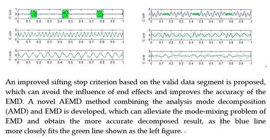
In this paper, a new sifting stop criterion was proposed based on valid data segments to solve the problem of sifting stop criteria in the EMD, and an improved method, namely AEMD, combined the analysis mode decomposition (AMD) and EMD. It was developed to solve the mode-mixing problem. The sifting stop criteria and AEMD proposed were applied to a simulation signal and an engineering case to illustrate the validity and superiority of the proposed method. The structure of the paper is as follows: Section 2 introduces the basic principles of EMD; Section 3 narrates the proposed sifting stop criteria based on valid data segment and compares it with the original one; in Section 4, the principle and steps of AEMD are expounded firstly, then applied to decompose simulation signals and a rotor vibration signal, and it is compared with the EMD and EEMD methods; finally, Section 5 draws a brief conclusion of current work.

2. Basic Principles of EMD

EMD refers to a “sifting” process, in which, the component with the smallest extreme time feature scale is sifted out firstly, then those with larger extreme time feature scales, and the component with the largest feature scales are finally sifted out. That is to say, the average frequency of IMF components obtained from the EMD is reduced gradually, and the main steps of the EMD are introduced as follows [24]:
(1) Firstly, identify all the local maximum points and minimum points of original signal x ( t ) , then match the upper and lower envelope spectrums of extreme points with cubic spline line respectively. Furthermore, ensure that the signal x ( t ) is between the upper and lower envelope spectrums; (2) calculate the local mean of upper and lower envelope spectrums, denoted as m 1 ; (3) calculate the first component h 1 ( t ) according to Equation (1):
h 1 ( t ) = x ( t ) m 1
(4) Judge that whether h 1 ( t ) can satisfy the conditions to be an IMF. If not, h 1 ( t ) should be treated as an original signal to repeat steps (1), (2) and (3) until h 1 ( t ) can meet the conditions, designated as C 1 ( t ) = h 1 ( t ) . C 1 ( t ) is the first IMF component after decomposition. (5) Separate C 1 ( t ) from the signal x ( t ) , i.e., r 1 ( t ) = x ( t ) c 1 ( t ) . (6) Treat r 1 ( t ) as an original signal to repeat steps (1)–(5), and after n cycles, n IMF components and 1 residual value r n ( t ) can be derived; i.e.,
{ r 2 = r 1 c 2 r 3 = r 2 c 3 r n = r n 1 c n
Then, the original signal x ( t ) can be expressed as:
x ( t ) = i = 1 n c i + r n
where ci refers to the ith IMF component and rn is the residual function.
This cycle comes to the end when rn becomes a monotonic function, but in the real decomposition process, when rn meets the conditions of monotonic function, the cycle number is usually large, and the number of IMF components will be too large. Furthermore, a mass of EMD tests have revealed that most of these final components obtained from EMD are false IMF components, without substantive physical significance. Thus, a good sifting stop criterion can not only improve the decomposition efficiency, but also increase the decomposition accuracy.
The stop criteria of decomposition process proposed by Huang was realized by limiting the standard deviation of the two adjacent IMFs and the sifting times are eventually controlled by the iteration threshold Sd [25]. In particular, Sd is defined as:
S d = t = 0 T [ h k ( t ) h k 1 ( t ) ] 2 h k 1 2 ( t )
where T refers to the time span of a signal, h k ( t ) and h k 1 ( t ) denote the two adjacent processing sequences in the process of EMD and the value of S d is usually between 0.2 and 0.3.
It is of great significance to determine reasonable iteration threshold S d . If the threshold is too small, the computational cost will increase greatly and the IMF components finally obtained will be of no significance; while if it is too large, it will be difficult to satisfy the condition of IMF.

3. The Sifting Stop Criteria Based on the Valid Data Segment

The sifting stop criteria of IMF proposed by Huang is valid for most cases, but there are some problems; it can be noted from Equation (3) that when hk(t) = 0, the iteration threshold will become an uncertain value. It is evidently inappropriate if the iteration threshold is used to control sifting number at the time. In addition, the sifting stop criteria ignored the influence of end effect. Consequently, the decomposition result may produce errors if the distorted endpoint data are adopted. In most cases, the end effect of EMD is obvious, though some effective measures will been taken to restrain it, the end effect still exists.
In this paper, an improved sifting stop criterion of IMF based on the valid data segment is proposed, where the valid data segment means the residual data segment after kicking out the distorted endpoint data. The sifting stop criteria fully consider the influence of end effect to sifting stop criteria, and only use the valid data segment to calculate the iteration threshold. The sifting stop criterion is expressed as follows:
If hk(t) is an IMF, it satisfies the following inequality:
δ < m ˜ k + 1 < δ
where m ˜ k + 1 denotes the valid data segment of the mean curve of upper envelope and lower envelope; δ represents the error threshold, which ranges from 0.01 to 0.1.
The EMD is applied to decompose a simulation signal respectively based on the proposed sifting stop criterion and the traditional one below. The simulation signal is
x ( t ) = x 1 ( t ) + x 2 ( t ) , t [ 0 , 1 ]
x 1 ( t ) = ( 1 + 0.5 sin ( 2 π 4 t ) ) 2 cos ( 2 π 80 t ) , x 2 ( t ) = sin ( 2 π 24 t )
The simulation signal consists of x1(t) and x2(t) (as shown in Figure 1, Figure 2 and Figure 3) are the decomposition results by using EMD based on the proposed sifting stop criterion and the traditional one, respectively. It is worth noting that the EMD can efficiently decompose the original signal by using the two sifting stop criteria, but it is clear from the two edges of these two figures that the decomposition result c1 and c2 in Figure 2 are more accurate than imf1 and imf2 in Figure 3, which show an evident end effect.
Figure 4 plots the vibration signal of a real gear with broken teeth. The number of gear teeth z = 75 ; module m = 2 ; the rotating frequency f = n 2 / 60 13.6 . EMD based on the proposed sifting stop criteria is used to decompose the vibration signal of a gear, and obtain five IMFs. The first IMF imf1 contains massive fault information of the gear. Note from its time domain graph (see Figure 5) that the waveform of imf1 presents an obvious modulation feature, and its cycle of modulation wave (T, approximately 0.074 s) accordingly had a frequency of about 13.6 Hz, which is exactly the rotating frequency of the faulty gear. Thus, it can be concluded that the fault information has been exacted from the vibration signal of the practical gears by using the proposed sifting stop criterion.

4. AEMD Method

4.1. Analytical Mode Decomposition (AMD) Method

AMD can separate the harmonic components of each frequency band from a multiband signal, its principle is as follows:
A signal x 0 ( t ) is separated into the two components by boundary frequency fb, one is the fast-changing signal xf(t) and another is slowly-changing signals xs(t):
x 0 ( t ) = x f ( t ) + x s ( t )
Their corresponding Fourier transforms Xf(ω), Xs(ω) have no overlap in the frequency band. The Hilbert transforms of cos ( 2 π f b t ) x 0 ( t ) and sin ( 2 π f b t ) x 0 ( t ) are as follows:
H [ cos ( 2 π f b t ) x 0 ( t ) ] = x s ( t ) H [ cos ( 2 π f b t ) ] + cos ( 2 π f b t ) H [ x f ( t ) ]
H [ sin ( 2 π f b t ) x 0 ( t ) ] = x s ( t ) H [ sin ( 2 π f b t ) ] + sin ( 2 π f b t ) H [ x f ( t ) ]
xs(t) and xf(t) can be derived from the above formulas:
x s ( t ) = sin ( 2 π f b t ) H [ cos ( 2 π f b t ) x 0 ( t ) ] cos ( 2 π f b t ) H [ sin ( 2 π f b t ) x 0 ( t ) ]
x f ( t ) = x 0 ( t ) x s ( t )
As aforementioned, the signal x 0 ( t ) is decomposed into xs(t) and xf(t) by using the analysis mode decomposition.

4.2. Steps of the AEMD Method

When the signal to be decomposed contains high-frequency intermittent signals or some similar compositions in time feature size, it is inevitable that the mode mixing appears in decomposition result by using EMD directly [11]. In this section, the AEMD that combines AMD with EMD is proposed to restrain the mode mixing in EMD. In particular, EMD is first applied to dispose the original signal, and then AMD is used to decompose these mixed modes. Then, these decomposed modes are reconstituted according to a certain principle. These reconstituted components show mode mixing phenomena alleviated. The specific steps are given as follows:
(1) EMD is applied to the original signal and obtain some IMFs and a residual component r;
(2) A fast Fourier transform (FFT) is conducted on IMFs, and the spectral diagrams of these IMFs are obtained. The first IMF1(t) with mode mixing is performed by AMD. The boundary frequency fb1 can be determined according to the spectrum. The average frequency of the two confused modes is used as the boundary frequency in this analysis. Then IMF1(t) is separated into the two signals c 1 ( t ) and c 1 ^ ( t ) by using AMD. c 1 ( t ) is the correction component of IMF1(t) and c 1 ^ ( t ) is the residual component of c 1 ( t ) . Thus, IMF1(t) can be expressed as follows:
I M F 1 ( t ) = c 1 ( t ) + c 1 ^ ( t )
(3) Add c 1 ^ ( t ) to the IMF2(t) and get the renewed IMF2(t), denoted as IMF*2(t). The boundary frequency fb2 can be obtained according to the amplitude spectrum of IMF*2(t). Then IMF*2(t) is decomposed into the two signals c 2 ( t ) and c 2 ^ ( t ) by using AMD. c 2 ( t ) is the correction component of IMF*2(t) and c 2 ^ ( t ) is the residual component of c 2 ( t ) . Similarly, IMF*2(t) is expressed as follows:
I M F 2 * ( t ) = c 2 ( t ) + c 2 ^ ( t )
(4) By that analogy, the similar approach is utilized to dispose all the subsequent IMF components with mode mixing. The final residual component c^k(t) is added to the residual error r and obtain the final residual error, denote as vk(t).

4.3. The Comparison of Simulation Signal Analysis by Different Methods

A simulation signal was decomposed by using EMD, EEMD and the proposed AEMD respectively, and their disposal results were compared, to demonstrate AEMD efficiency and superiority. The simulation signal x(t) is:
x ( t ) = x 1 ( t ) + x 2 ( t ) + x 3 ( t ) ; t [ 0 , 1 ]
x 1 ( t ) = { 0.8 cos ( 600 π t ) ; 0.12 t 0.18 0.9 cos ( 600 π t ) ; 0.42 t 0.48 0.8 cos ( 600 π t ) ; 0.75 t 0.81 0 ; else
x 2 ( t ) = 2 cos ( 60 π t ) ; t [ 0 , 1 ] x 3 ( t ) = 2.5 cos ( 28 π t ) ; t [ 0 , 1 ]
The simulation signal is shown in Figure 6. The decomposition result of EMD, in Figure 7, shows more serious mode mixing. For the first mode, the high frequency intermittency signal c1(t) is confused with the sinusoidal signal at 30 Hz, for the second mode c2(t), the sinusoidal signal at 30 Hz with the sinusoidal signal at 14 Hz. The third and fourth modes are false IMF components. The decomposition result of EEMD is imf1, imf2, imf3, imf4, as shown in Figure 8, with ensemble average number N = 30, and the amplitude of noise is set as 0.01 standard deviation of the original signal. The decomposition result of AEMD is shown in Figure 9. A successful decomposition result should distinctly obtain the several components of the original signal. In order to compare the results of decomposition results by these different methods, the green lines in Figure 7, Figure 8 and Figure 9 represent the several components of the original signal; The blue lines represent the composition results by these different methods. Table 1 lists the run time by these three methods using the same computer.
Note from Figure 7, Figure 8 and Figure 9 that the goodness of fit between the blue line and green line by EEMD and AEMD methods is higher than that of EMD. The comparison of these three methods reveals that EEMD and AEMD can restrain effectively the mode confusion phenomena, but the running time of EEMD is much longer than those of AEMD and EMD, because the EEMD method adds white noise to original signals to alleviate mode mixing problem, which makes the decomposition process more complex and time-consuming. The executed time of EMD is approximately equal with AEMD’s, but it has inevitable mode mixing problem. Thus, AEMD has shown certain comprehensive advantages in alleviating mode mixing and making decomposition efficient.

4.4. Case Study

Figure 10 presents the experimental device to simulate the local rubbing fault of rotors, during which the rotate-speed was at 300 RPM, controlled by the inputted motor. The displacement sensor that was horizontally installed was employed to sample the vibration signals, with sampling frequency 4k Hz. Figure 11 plots the vibration signal of a practical rotor system with rub-fault. The decomposition result for the vibration signal by using the EMD and the AEMD are shown as Figure 12 and Figure 13, respectively. Figure 14a,b is the spectrum diagram by fast Fourier transform (FFT) for the composition results of EMD and AEMD, respectively.
Note from Figure 12 and Figure 14a that the mode mixing problem still distinctly exists in the decomposition results by EMD. In the imf2 diagram, the characteristic frequency of the rotor rubbing fault is confused in multiple frequencies, caused by the slight rubbing fault of the rotor, which affects the identification for the fault. In the imf3 diagram, the triple frequency of the characteristic frequency of the rotor rubbing fault—150 Hz is nearly invisible, which is mixed in the fundamental frequency of the rotor rubbing fault—50 Hz.
In addition, note from Figure 13 and Figure 14b that the tripling frequency 150 Hz and ten times frequency—500 Hz of the characteristic frequency of the rotor rubbing fault are distinctly decomposed. This spectrum character with multiple higher harmonics is in accordance with the slight rubbing fault of the rotors. Thus, the characteristic frequency of the rotor rubbing fault is successfully obtained by AEMD, though there is still slighter mode mixing.

5. Conclusions

In this paper, an improved sifting stop criterion based on valid data segment was proposed. Compared with the traditional one, results indicated that the newly proposed sifting stop criterion avoids the influence of end effects and improves the correctness of the EMD. In addition, a novel method, namely AEMD, which combines the AMD and EMD, was developed to solve the mode mixing problem of EMD. Model comparison was conducted between the proposed method and the EEMD. It is worth mentioning that both the AEMD and EEMD can effectively restrain the mode mixing, but the AEMD needs less execution time than that of EEMD. The proposed method overcomes some shortcomings of EMD to some extent and makes it better for use in the fault diagnosis of rotating machinery. However, the proposed method has certain imitations; the boundary frequency of AMD method requires human intervention, which means worse adaptivity than EMD. It can achieve better results for more simple signals, but its advantage is not obvious for complex engineering signals, since they take more time than EMD.

Author Contributions

Z.C. conceived the methodology, conducted the research and wrote the original draft. B.L. performed the programming to fulfil the method and edited the manuscript. X.Y. collected data and analyzed the data. H.Y. investigated the experiment and discussed the results.

Funding

This research was funded by the National Natural Science Foundation of China grant number 11672070.

Conflicts of Interest

We declare no conflict of interest.

References

  1. Chen, Z.; Cao, S.; Mao, Z. Remaining useful life estimation of aircraft engines using a modified similarity and supporting vector machine (SVM) approach. Energies 2017, 11, 28. [Google Scholar] [CrossRef]
  2. Han, J.; Ji, G.Y. Gear Fault Diagnosis Based on Improved EMD Method and the Energy Operator Demodulation Approach. J. Changsha Univ. Sci. Technol. 2015, 12, 66–71. [Google Scholar]
  3. Yang, Y.F.; Wu, Y.F. Application of Empirical Mode Decomposition in the Analysis of Vibration; National Defence of Industry Press: Beijing, China, 2013; pp. 17–45. [Google Scholar]
  4. Huang, D.S. The Method of False Modal Component Elimination in Empirical Mode Decomposition. Vibration. Meas. Diagn. 2011, 31, 381–384. [Google Scholar]
  5. Wang, L. Fault Diagnosis of Rotor System Based on EMD-Fuzzy Entropy and SVM. Noise Vib. Control 2012, 6, 172–173. [Google Scholar]
  6. Ben Ali, J.; Fnaiech, N.; Saidi, L.; Chebel-Morello, B.; Fnaiech, F. Application of empirical mode decomposition and artificial neural network for automatic bearing fault diagnosis based on vibration signals. Appl. Acoust. 2015, 89, 16–27. [Google Scholar] [CrossRef]
  7. Xue, X.; Zhou, J.; Xu, Y.; Zhu, W.; Li, C. An Adaptively Fast Ensemble Empirical Mode Decomposition Method and Its Applications to Rolling Element Bearing Fault Diagnosis. Mech. Syst. Sig. Process. 2015, 62–63, 444–459. [Google Scholar] [CrossRef]
  8. Yu, D.J.; Cheng, J.S. The Hilbert-Huang Transform Method in Mechanical Fault Diagnosis; Science Press: Beijing, China, 2006; pp. 179–190. [Google Scholar]
  9. Cheng, J.; Xu, Y.L. Application of HHT Method in Structural Modal Parameter Identification. J. Vib. Eng. 2003, 16, 383–387. [Google Scholar]
  10. Cheng, J.; Yang, Y. The application of EMD Method in Local Touch Friction Fault Diagnosis of Rotor. Vibration. Meas. Diagn. 2006, 26, 24–27. [Google Scholar]
  11. Rilling, G.; Flandrin, P. One or Two Frequencies? The Empirical Mode Decomposition Answers. IEEE Trans. Signal Process. 2008, 56, 85–95. [Google Scholar] [CrossRef]
  12. Dou, D.Y.; Zhao, Y.K. Application of Ensemble Empirical Mode Decomposition in Failure Analysis of Rotating Machinery. Trans. Chin. Soc. Agric. Eng. 2010, 26, 190–196. [Google Scholar]
  13. Pustelnik, N.; Borgnat, P.; Flandrin, P. Empirical mode decomposition revisited by multicomponent non-smooth convex optimization. Signal Process. 2014, 102, 313–331. [Google Scholar] [CrossRef]
  14. Lei, Y.G.; He, Z.J.; Zi, Y.Y. Application of the EEMD Method to Rotor Fault Diagnosis of Rotating Machinery. Mech. Syst. Signal Process. 2009, 23, 1327–1338. [Google Scholar] [CrossRef]
  15. Zhao, J.P. Study on the Effects of Abnormal Events to Empirical Mode Decomposition Method and the Removal Method for Abnormal Signal. J. Ocean Univ. Qingdao 2001, 31, 805–814. [Google Scholar]
  16. Deering, R.; Kaiser, J.F. The Use of a Masking Signal to Improve Empirical Mode Decomposition. Acoust. Speech Signal Process. ICASSP 2005, 4, 485–488. [Google Scholar]
  17. Hu, A.J. Research on the Application of Hilbert-Huang Transform in Vibration Signal Analysis of Rotating Machinery; North China Electric Power University: Bao Ding, Hebei, China, 2008. [Google Scholar]
  18. Wu, Z.; Huang, N.E. Ensemble Empirical Mode Decomposition: A Noise-Assisted Data Analysis Method. Adv. Adapt. Data Anal. 2009, 1, 1–41. [Google Scholar] [CrossRef]
  19. Chen, G.D.; Wang, Z.C. A Signal Decomposition Theorem with Hilbert Transform and Its Application to Narrow Band Time Series with Closely Spaced Frequency Components. Mech. Syst. Signal Process. 2012, 28, 258–279. [Google Scholar] [CrossRef]
  20. Lei, Y.G.; Kong, D.T. Adaptive Ensemble Empirical Mode Decomposition and Application to Fault Detection of Planetary Gear Boxes. J. Mech. Eng. 2014, 50, 64–70. [Google Scholar] [CrossRef]
  21. Zheng, J.D.; Cheng, J.S.; Yang, Y. Partly Ensemble Empirical Mode Decomposition: An Improved Noise-Assisted Method for Eliminating Mode Mixing. Signal Process. 2014, 96, 362–374. [Google Scholar] [CrossRef]
  22. Hu, J.S.; Yang, S.X. Energy-Based Stop Condition of Empirical Mode Decomposition of Vibration Signal. J. Vib. Meas. Diagn. 2009, 29, 19–22. [Google Scholar]
  23. Mohammad, S.H.; Siamak, E.K.; Mohammad, S.S. Quantitative diagnosis for bearing faults by improving ensemble empirical mode decomposition. ISA Trans. 2018, 83, 261–275. [Google Scholar]
  24. Yang, Y.; Yu, D.J.; Cheng, J.S. A Roller Bearing Fault Diagnosis Method Based on EMD Energy Entropy and ANN. J. Sound Vib. 2006, 294, 269–277. [Google Scholar]
  25. Huang, N.E.; Shen, Z.; Long, S.R.; Wu, M.C.; Shih, H.H.; Zheng, Q.; Yen, N.C.; Tung, C.C.; Liu, H.H. The Empirical Mode Decomposition and the Hilbert Spectrum for Nonlinear and Non-stationary Time Series Analysis. Proc. R. Soc. Lond. A 1998, 454, 903–995. [Google Scholar] [CrossRef]
Figure 1. The simulation signal and its two components.
Energies 12 03077 g001
Figure 2. The result of empirical mode decomposition (EMD) method using the sifting criterion based on the valid data segment.
Energies 12 03077 g002
Figure 3. The result of EMD method using the sifting criterion proposed by Huang.
Energies 12 03077 g003
Figure 4. The vibration signal of gear with broken teeth.
Energies 12 03077 g004
Figure 5. The first IMF of EMD for the vibration signal with broken teeth.
Energies 12 03077 g005
Figure 6. The time domain chart of simulation signal x(t).
Energies 12 03077 g006
Figure 7. The decomposition result of the simulation signal by EMD.
Energies 12 03077 g007
Figure 8. The decomposition result of the simulation signal by ensemble empirical mode decomposition (EEMD).
Energies 12 03077 g008
Figure 9. The decomposition result of the simulation signal by AEMD (combined AMD and EMD).
Energies 12 03077 g009
Figure 10. The experimental device for simulating local rubbing fault of rotors.
Energies 12 03077 g010
Figure 11. The vibration signal of rub-fault for rotors.
Energies 12 03077 g011
Figure 12. The decomposition result for the vibration signal of rub-fault by EMD.
Energies 12 03077 g012
Figure 13. The decomposition result for the vibration signal of rubbing-fault by AEMD.
Energies 12 03077 g013
Figure 14. (a) The spectrum of intrinsic mode functions (IMFs) by EMD. (b) The spectrum of IMFs by AEMD.
Energies 12 03077 g014
Table 1. The running time of the three methods (unit: seconds).
MethodFirstSecondThirdFourthFifthSixth
EMD1.39881.38601.39301.38461.38201.3940
EEMD41.487544.838344.180042.848043.232144.024
AEMD1.40271.38321.38431.39341.38801.3848

