A Minimum Side-Lobe Optimization Window Function and Its Application in Harmonic Detection of an Electricity Gird

Abstract

Several window functions are currently applied to improve the performance of the discrete Fourier transform (DFT) harmonic detection method. These window functions exhibit poor accuracy in measuring the harmonic contents of a signal with high-order and weak-amplitude components when the power frequency fluctuates within a small range. In this paper, a minimum side-lobe optimization window function that is aimed at overcoming the abovementioned issue is proposed. Moreover, an improved DFT harmonic detection algorithm based on the six-term minimum side-lobe optimization window and four-spectrum-line interpolation method is proposed. In this context, the minimum side-lobe optimization window is obtained by optimizing the conventional cosine window function according to the optimization rules, and the characteristics of the new proposed window are provided to analyze its performance. Then, the proposed optimization window function is employed to improve the DFT harmonic detection algorithm based on the six-term minimum side-lobe optimization window and four-spectrum-line interpolation method. The proposed technique is used to detect harmonics of an electricity gird in which the six-term minimum side-lobe optimization window is utilized to eliminate the influence of spectrum leakage caused by nonsynchronous sampling of signal processing. The four-spectrum-line interpolation method is employed to eliminate or mitigate the fence effect caused by the inherent measurement error of the DFT method. Simulation experiments in two complex conditions and an experiment test are carried out to validate the improved performance of the proposed window. Results reveal that the six-term minimum side-lode optimization window has the smallest peak side lobe when compared with existing windows, which can effectively reduce the interaction influence of spectrum leakage, improve the measurement accuracy of the DFT harmonic detection method, and meet the standard requirement of harmonic measurement in complex situations.

1. Introduction

As new energy generation technology is widely applied to the electricity grid via the power electronics interface, power quality has become a significant issue with the continuous increase in voltage and current harmonics [1,2,3]. In addition to their adverse impact on power quality, complex harmonics introduce significant current and voltage measurement errors and have threatening impacts on the security and stability of electricity gird [4,5,6,7,8]. Therefore, a prioritized task on the agenda of electricity utilities is to detect harmonics accurately as a first step to adopt cost-effective measures to eliminate harmonic pollution.

The conventional discrete Fourier transform (DFT) harmonic detection method is widely used in practical applications as it is easily embedded into the harmonic measurement system in power grids [8,9,10]. However, during the procedure of signal processing sampling, the harmonic signal is cut off into constant length ones. Because of the influence of power grid frequency fluctuation, the process of DFT exhibits incomplete period cutoff and nonsynchronous sampling, which results in spectrum leakage that causes inaccuracy in the harmonic measurement [11,12,13]. Moreover, as the DFT harmonic detection method obtains the frequency spectrum in the discrete frequency domain after processing the signal dispersion, the fluctuation of power frequency makes it difficult to coincide with the true frequency spectrum of the harmonic signal, which leads to a measurement error referred as the fence effect [14,15].

The method of applying a window function to weaken the spectrum leakage and reduce the spectrum interference between harmonic signals has been proposed in the literature [16,17,18]. Conventional window functions adopted in the practical applications include Hanning window, Blackman window, and Blackman–Harris window [19,20,21]. However, the conventional window functions show poor performance in measuring the harmonic signal with high-order and weak-amplitude components. Employing spectrum-line interpolation methods such as the double-spectrum-line interpolation method can reduce the measurement error caused by the fence effect. This method is based on calculating a correcting frequency deviation by weighting the highest and sub-high spectrum lines near the peak point in the frequency domain and then adjusting the amplitude, phase, and frequency, so as to decrease the influence of the fence effect [22,23]. A synopsis of the harmonic detection methods proposed in the literature, depending on the type of analysis, is presented in

Table 1. Synopsis of harmonic detection methods. CDFT—conventional discrete Fourier transform harmonic detection method; WDFT—windowed discrete Fourier transform harmonic detection method; and SDFT—spectrum-line interpolation discrete Fourier transform harmonic detection method.

Method	Advantages	Drawbacks
CDFT	Widely used in practical applications and is easy to embed into the harmonic measurement system	Signal process belongs to incomplete period cutoff and nonsynchronous sampling, and the harmonic detection accuracy is influenced by spectrum leakage and fence effect
WDFT	Can weaken spectrum leakage and reduce the spectrum interference between harmonics	Conventional windows show poor performance in measuring the harmonic signal with high-order and weak-amplitude components
SDFT	Can reduce the measurement error caused by fence effect	Only two spectrum lines the near peak point are considered for the double-spectrum-line interpolation method but abundant spectrum information near the actual frequency point is ignored

.

In this paper, a minimum side-lobe optimization new window function aimed at enhancing the accuracy of harmonic detection is introduced. The paper is structured as follows: In Section 2, a minimum side-lobe optimization window function is proposed and analyzed. In Section 3, an improved DFT harmonic detection algorithm based on the six-term minimum side-lobe optimization window and four-spectrum-line interpolation method is elaborated throughout its application to detect harmonics of an electricity grid. Two simulations in complex conditions are carried out to validate the feasibility of the proposed algorithm in Section 4 and the experiment test is implemented in Section 5. Finally, conclusions are drawn in Section 6 and an Abbreviation table that shows the abbreviations in the article is presented in Abbreviations.

2. Proposed Minimum Side-Lobe Optimization Window

2.1. Optimization Rules of the Minimum Side-Lobe Optimization Window

The combined cosine window function is used to reduce the influence of spectrum leakage. The time domain mathematical expression of the combined cosine window function can be written as:

$$w_M(t)={\displaystyle \sum _{i=0}^{K-1}{(-1)}^i}{a}_i\cos (2\pi it/N),$$

(1)

where $K$ is the highest term of the combined cosine window function, $a_i$ is the coefficient of the window function, and $N$ is the sampling point.

The n-order derivative of Equation (1) is:

$$w_M{}^n(t)={(2\pi )}^n{\displaystyle \sum _{i=0}^{K-1}{i}^n}{a}_i\cos (2\pi it/N+\pi n/2).$$

(2)

The performance of the combined cosine window is determined by the width of the main lobe and the peak value of the side lobe. When the main-lobe width of the window becomes smaller, the frequency resolution becomes larger; the small peak value of the side lobe improves the performance of the side lobe of the window and the spectrum leakage suppression ability.

Therefore, in order to optimize the side-lobe performance of the combined cosine window function, the following procedure will be adopted. In order to obtain the minimum side-lobe value, the following two rules are applied:

Rule 1. The coefficients of the combined cosine window function must sum up to unity, i.e.,

$${\displaystyle \sum _{i=0}^{K-1}{a}_i}=1.$$

(3)

Rule 2. In order to obtain the smallest side-lobe value among the combined cosine window with the same terms, zero points must be added to the first to fifth side lobe of the window function in the frequency domain. Meanwhile, it is necessary to make the n-order derivative of the combined cosine window function continuous. According to this rule, a constraint condition can be written as:

$${\displaystyle \sum _{i=0}^{K-1}{(-1)}^i{i}^n{a}_i}=0.$$

(4)

From Equations (3) and (4), it can be revealed that the performance of the window function is determined by the term of the combined cosine window ($K$), the coefficient of the window function ($a_i$), and the derivative order ($n$). When the term of the cosine window function increases, the side-lobe value decreases but the width of the main lobe also increases consequently. Therefore, the number of the cosine window terms should not be too large, generally it is taken as $K=1~6$.

For $K=1~6$ and based on the constraint equations, the minimum side-lobe value of the cosine window can be obtained. Therefore, it can be called as minimum side-lobe optimization window (MSOW). The window function coefficient can be worked out as shown in

Table 2. Coefficient of the minimum side-lobe optimization window (MSOW).

$\mathit{K}$	1	2	3	4	5	6
Window Coefficient	1-Term MSOW	2-Term MSOW	3-Term MSOW	4-Term MSOW	5-Term MSOW	6-Term MSOW
a0	1	5.3835539 × 10−1	4.2438009 × 10−1	3.6358193 × 10−1	3.2321538 × 10−1	2.9355790 × 10−1
a1	----	4.6164461 × 10−1	4.9734064 × 10−1	4.8917744 × 10−1	4.7149214 × 10−1	4.5193577 × 10−1
a2	----	----	7.8279271 × 10−2	1.3659951 × 10−1	1.7553413 × 10−1	2.0141647 × 10−1
a3	----	----	----	1.0641122 × 10−2	2.8496990 × 10−2	4.7926109 × 10−2
a4	----	----	----	----	1.2613571 × 10−3	5.0261964 × 10−3
a5	----	----	----	----	----	1.3755557 × 10−4

, and when $K=1$, the window is called a rectangular window.

2.2. Performance Analysis of the Minimum Side-Lobe Optimization Window

Discrete Fourier transform is applied to Equation (1) and the frequency domain function can be written as:

$$W_M(\omega )={\displaystyle \sum _{i=0}^{K-1}{(-1)}^i\frac{a_i}{2}}(R(\omega -\frac{2\pi i}{N})+R(\omega +\frac{2\pi i}{N})),$$

(5)

where $R(\omega )=\frac{\sin (\omega N/2)}{\sin (\omega /2)}{e}^{-j\frac{N-1}{2}\omega }$ is the frequency domain function of the rectangular window. Therefore, the logarithmic amplitude–frequency characteristic function can be obtained as:

$$W_{M(dB)(\omega )}=20\lg \left|\frac{W_M(\omega )}{W_M(0)}\right|.$$

(6)

In order to analyze the time and frequency domain characteristics of the minimum side-lobe optimization window, the window coefficients in Table 2 are substituted into Equations (5) and (6) to obtain its logarithmic amplitude–frequency characteristic. The time domain and frequency domain characteristics of the minimum side-lobe optimization window are shown in Figure 1. Based on the expressions of the minimum side-lobe optimization window, the side-lobe value and main-lobe width are derived and summarized in

Table 3. Performance of the minimum side-lobe optimization window.

Window	Side-Lobe Value/dB	Main-Lobe Width
2-term MSOW	−43	$8\pi /\mathrm{N}$
3-term MSOW	−72	$12\pi /\mathrm{N}$
4-term MSOW	−98	$16\pi /\mathrm{N}$
5-term MSOW	−125	$20\pi /\mathrm{N}$
6-term MSOW	−153	$24\pi /\mathrm{N}$

.

The side-lobe characteristics of the six-term minimum side-lobe optimization window are compared with the existing six-term combined cosine window, which is shown in Figure 2a. In order to validate the improved side-lobe performance of the six-term minimum side-lobe optimization window, conventional windows such as Hamming window, Blackman window, Nuttall window, and the comparison of spectrum characteristics are shown in Figure 2b.

From the window characteristic study of the proposed minimum side-lobe optimization window and the existing conventional windows, the conclusions can be obtained as:

(1)

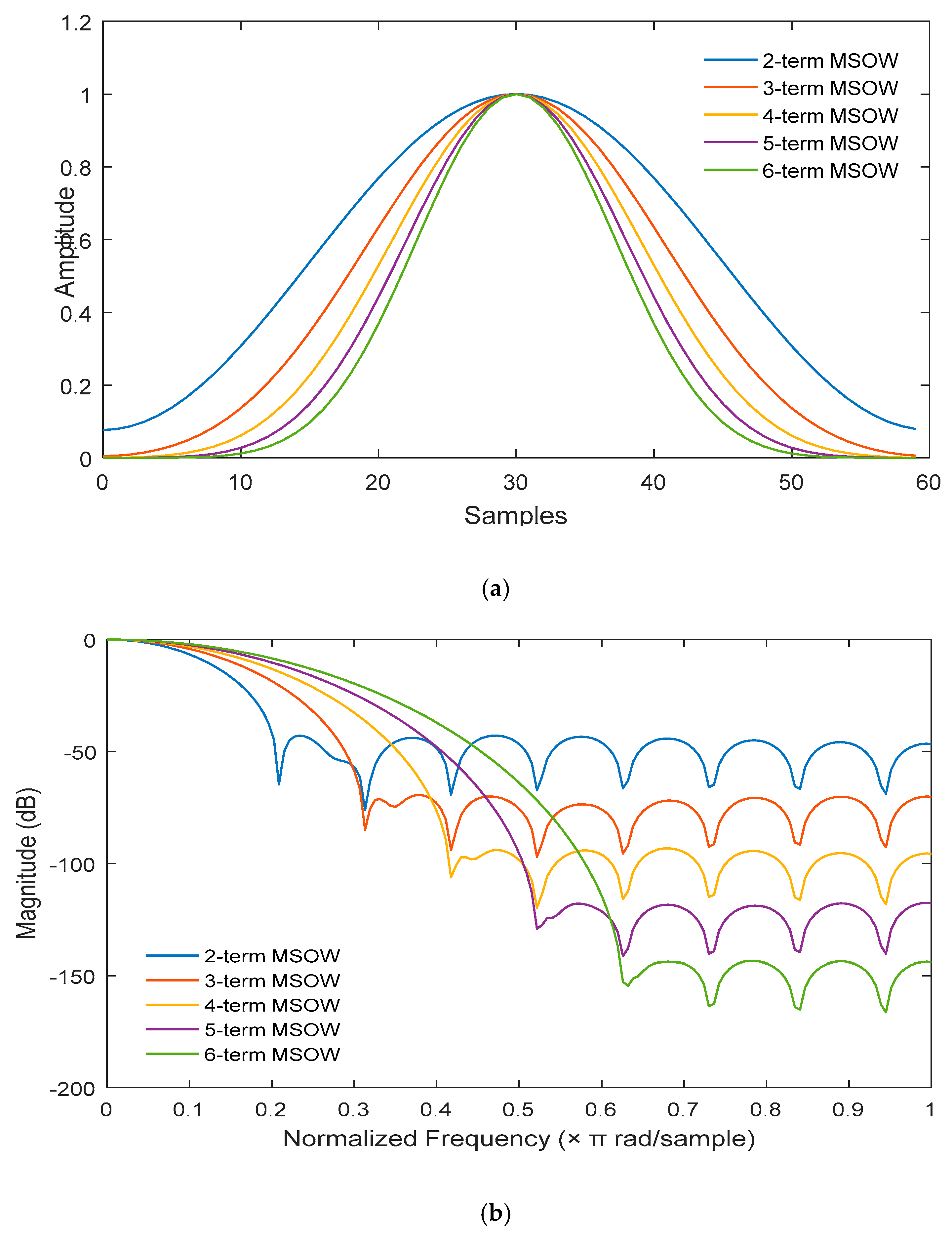
As can be seen from Figure 1b, the side-lobe peak value of the MSOW decreases significantly as the term of the window increases, but with the increase of the main-lobe width, which will reduce the frequency resolution. Therefore, the number of the window term cannot be large. The frequency resolution of the six-term MSOW can meet the standard requirement of harmonic measurement. Thus, the six-term MSOW is adopted and applied in harmonics analysis in complex situations with high-order and weak-amplitude in the power gird.

(2)

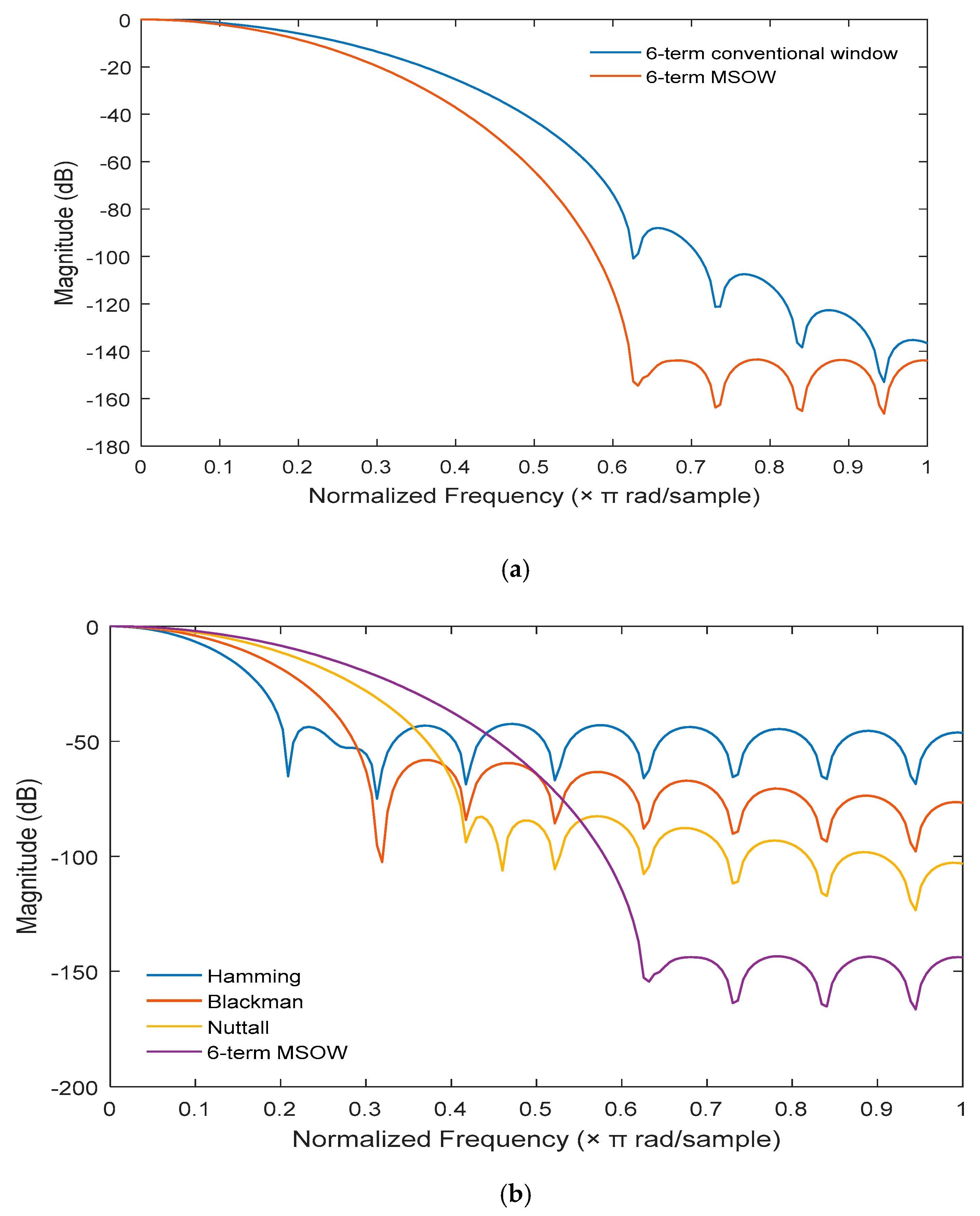
As can be seen from Figure 2a, the side-lobe peak value of the six-term MSOW is −153 dB, while that of the six-term conventional cosine window is −88 dB, which proves that the side-lobe peak value can be significantly reduced after window optimization. Besides, the two windows in Figure 2a have the same main-lobe width, so it has no influence on the frequency resolution after window optimization.

(3)

As can be seen from Figure 2b, the side-lobe peak value of the six-term MSOW is smaller than that of the conventional Hamming window, Blackman window, and Nuttall window. The spectrum leakage of the six-term MSOW is smaller than that of the other three windows and the spectrum information is concentrated in the main-lobe region, which can significantly suppress the mutual interference of spectrum leakage between harmonics.

3. Proposed Improved DFT Harmonic Detection Algorithm

According to the proposed minimum side-lobe optimization window, an improved DFT harmonic detection algorithm based on the six-term minimum side-lobe optimization window and four-spectrum-line interpolation method is proposed and presented in this section. The principle of the proposed algorithm and the derivation process of harmonic parameters are described and elaborated below.

3.1. Principle of Proposed Improved DFT Harmonic Detection Algorithm

A harmonic signal in the electricity gird in time-domain form is given as:

$$x(n)={\displaystyle \sum _{m=1}^M{A}_m\sin (2\pi n{f}_m/f_s+{\phi }_m)},$$

(7)

where $M$ is the highest order of harmonic contents in the signal x(n) and $f_s$ is the sampling frequency. $A_m$, ${\phi }_m$, and $f_m$ are, respectively, the amplitude, phase, and frequency of the m-th harmonic.

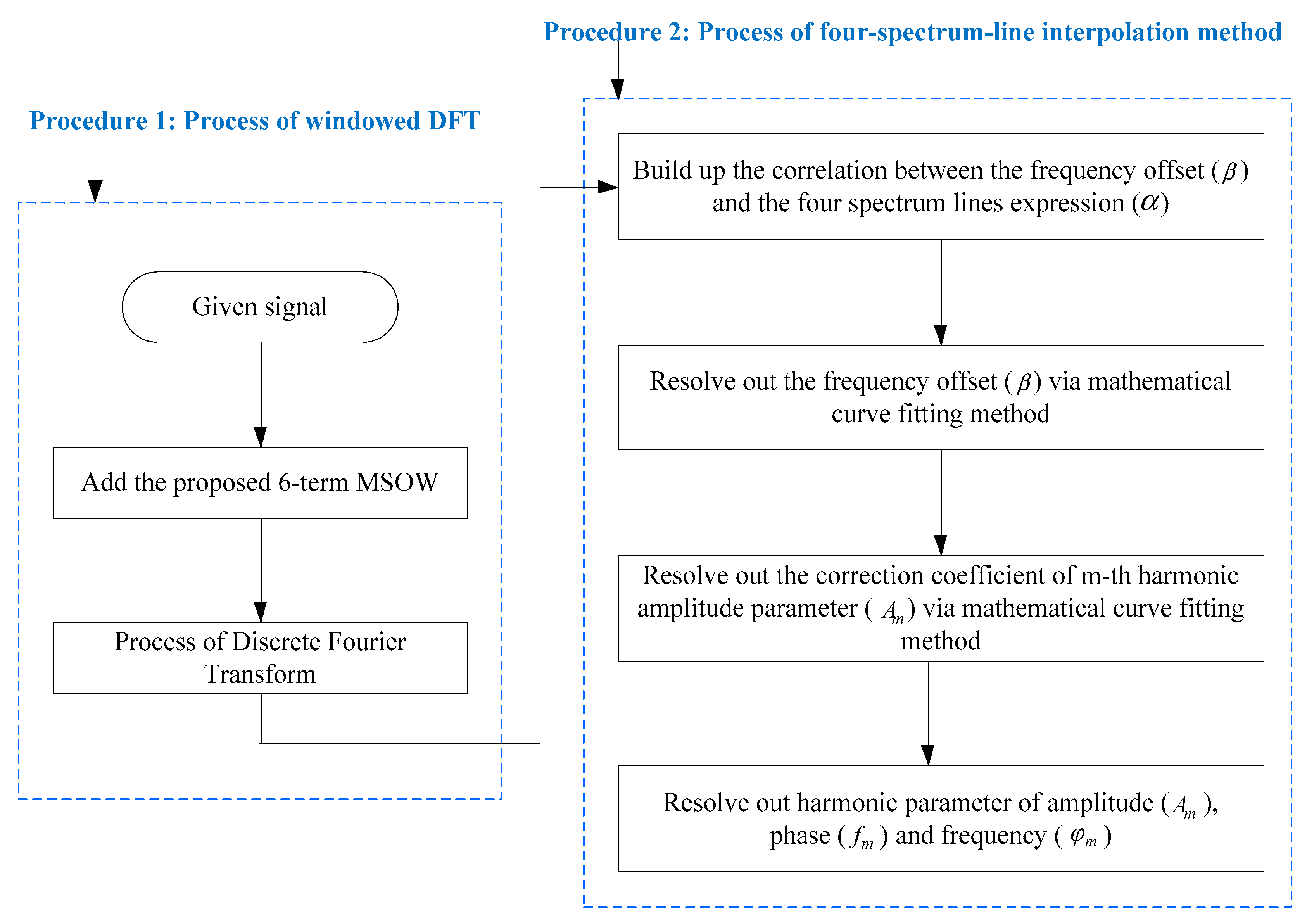
3.1.1. Procedure 1: Process of Windowed DFT

Step 1. Add the proposed six-term MSOW: The given signal $x(n)$ is processed by adding the proposed six-term MSOW, and the time-domain function after adding the six-term MSOW can be expressed as:

$$x_M(n)=x(n)w_M(n).$$

(8)

Step 2. Process of DFT: Discrete Fourier transform (DFT) is applied to Equation (8) to obtain its frequency-domain function, which is expressed as in Equation (9), where $\Delta f$ denotes the frequency resolution, $\Delta f=f_s/N$. Because the signal $x_M(n)$ is a real singular function and its discrete Fourier transform is an imaginary singular function, there are also existing spectrum lines at the corresponding negative frequency points. Therefore, the side-lobe effect at the negative frequency points can be neglected for analysis and Equation (9) can be simplified as in Equation (10).

$$X_M(\lambda )={\displaystyle \sum _{m=1}^M\frac{A_m}{2j}}[e^{j{\phi }_m}{W}_M(\lambda -f_m/\Delta f)-e^{-j{\phi }_m}{W}_M(\lambda +f_m/\Delta f)\begin{array}{cc}& \lambda =0,1,\cdots ,N-1\end{array},$$

(9)

$$X_M(\lambda )={\displaystyle \sum _{m=1}^M\frac{A_m}{2j}}{e}^{j{\phi }_m}{W}_M(\lambda -f_m/\Delta f)\begin{array}{cc}& \lambda =0,1,\cdots ,N-1\end{array}.$$

(10)

The influence of the other harmonics on the m-th harmonic can be neglected here in order to analyze the principle of the proposed algorithm, and thus Equation (10) can be simplified as in Equation (11). Where, $W_M(\lambda )$ is the discrete frequency-domain function of the six-term MSOW, which can be expressed as in Equation (12). The absolute values of Equations (11) and (12) are shown in Equations (13) and (14), respectively.

$$X_M(\lambda )=\frac{A_m}{2j}{e}^{j{\phi }_m}{W}_M(\lambda -f_m/\Delta f)\begin{array}{cc}& \lambda =0,1,\cdots ,N-1\end{array},$$

(11)

$$W_M(\lambda )=\frac{N}{\pi }\sin (\pi \lambda )e^{j\frac{\pi }{N}\lambda }{e}^{-j\pi \lambda }{\displaystyle \sum _{i=0}^{i=5}{(-1)}^i}\frac{a_i\lambda }{{\lambda }^2-i^2}.$$

(12)

$$\left|X_M(\lambda )\right|=\frac{A_m}{2}\left|W_M(\lambda -f_m/\Delta f)\right|,$$

(13)

$$\left|W_M(\lambda )\right|=\frac{N}{\pi }\left|\sin (\pi \lambda ){\displaystyle \sum _{i=0}^{i=5}{(-1)}^i}\frac{a_i\lambda }{{\lambda }^2-i^2}\right|.$$

(14)

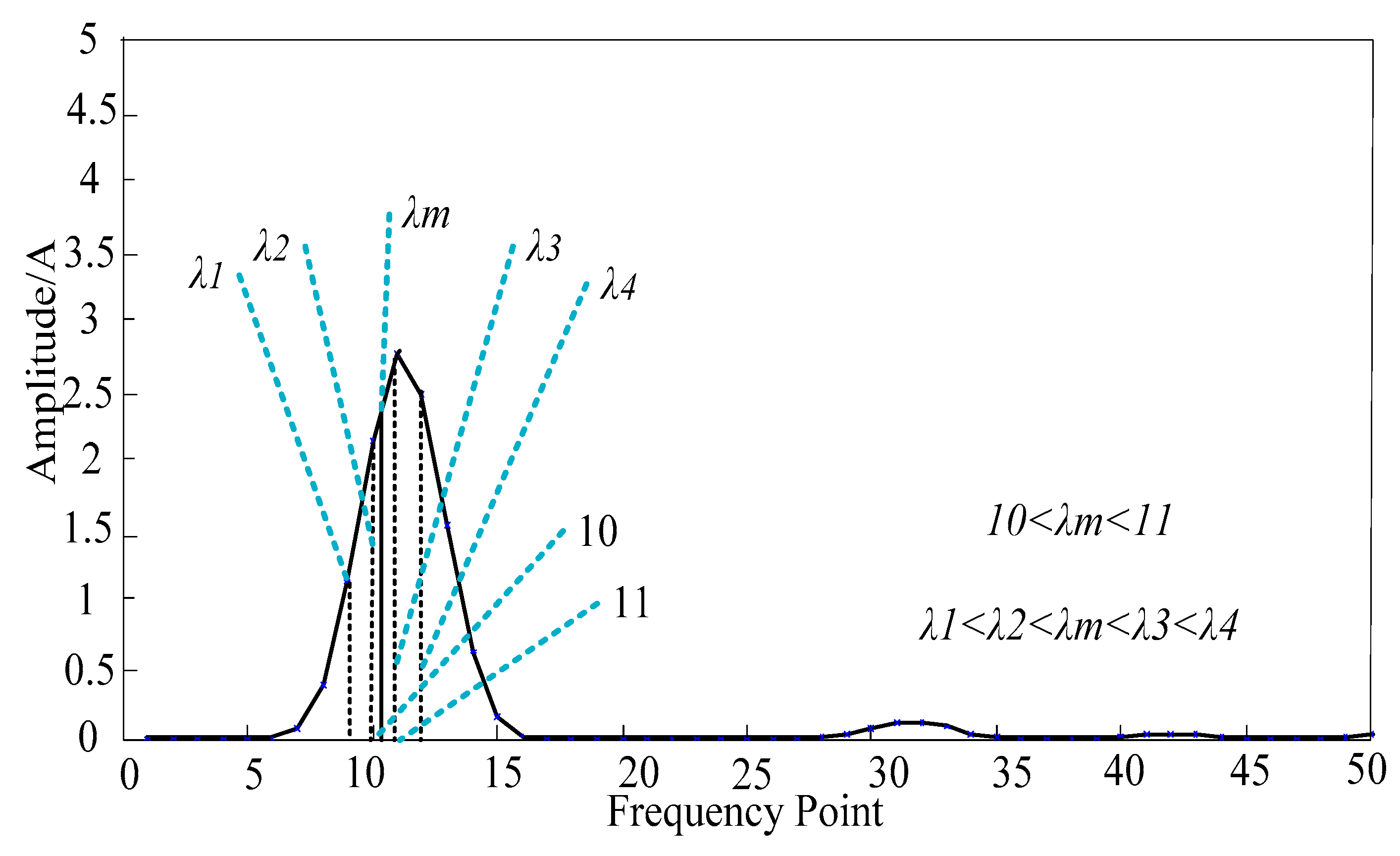
3.1.2. Procedure 2: Process of Four-Spectrum-Line Interpolation Method

During the process of DFT, the nonsynchronous signal sampling causes the fence effect, which leads to a significant harmonic measurement error. Therefore, it is difficult for the detection frequency of the m-th harmonic to be just equal to the real value at the integer frequency point as ${\lambda }_m=f_m/\Delta f$ is not an integer number. For example, in Figure 3 which gives the schematic diagram of harmonic signal spectrum, ${\lambda }_m$ is usually not equal to 10, $10<{\lambda }_m<11$.

The double-line interpolation method has been proposed to decrease the influence of the fence effect [24]. Applying the double-line interpolation method, the harmonic parameters can be corrected by weighting the maximum and sub-maximum lines near the peak point of the m-th harmonic frequency, in which the maximum and sub-maximum line is close to the actual frequency point. However, the double-line interpolation method has a disadvantage as it considers the two spectrum lines near the peak point while ignoring the abundant spectrum information near the actual frequency point. Thus, it exhibits poor harmonic measurement accuracy when measuring harmonic signals with high order and weak amplitude. Therefore, in this paper, a four-spectrum-line interpolation method is proposed, which takes full account of the spectrum information. The process of the four-spectrum-line interpolation method is presented in the below steps.

Step 1. Build up the correlation between the frequency offset ($\beta$) and the four spectrum lines expression ($\alpha$).

Figure 3 gives the schematic diagram of harmonic signal spectrum. First, the peak frequency point of the m-th harmonic is set as ${\lambda }_m$, its corresponding adjacent four spectrum lines are ${\lambda }_{m1}$, ${\lambda }_{m2}$, ${\lambda }_{m3}$, and ${\lambda }_{m4}$, and the amplitudes of the four spectrum lines are, respectively, $y_{m1}=\left|X_M({\lambda }_{m1})\right|$, $y_{m2}=\left|X_M({\lambda }_{m2})\right|$, $y_{m3}=\left|X_M({\lambda }_{m3})\right|$, and $y_{m4}=\left|X_M({\lambda }_{m4})\right|$. Where, the position relationship of the four spectrum lines is ${\lambda }_{m1}<{\lambda }_{m2}<{\lambda }_{m3}<{\lambda }_{m4}$, in which ${\lambda }_{m2}={\lambda }_{m1}+1$, ${\lambda }_{m3}={\lambda }_{m2}+1$, and ${\lambda }_{m4}={\lambda }_{m3}+1$.

The frequency offset is set as $\beta ={\lambda }_m-{\lambda }_{m2}-0.5$, where the range of $\beta$ is $\beta \in [-0.5,-0.5]$, and the four spectrum lines expression $\alpha$ is set as:

$$\alpha =\frac{(y_{m3}+y_{m4})-(y_{m1}+y_{m2})}{y_{m1}+y_{m2}+y_{m3}+y_{m4}},$$

(15)

$$\alpha =\frac{(\left|W_M(-\beta +0.5)\right|+\left|W_M(-\beta +1.5)\right|)-(\left|W_M(-\beta -0.5)\right|+\left|W_M(-\beta -1.5)\right|)}{\left|W_M(-\beta +0.5)\right|+\left|W_M(-\beta +1.5)\right|+\left|W_M(-\beta -0.5)\right|+\left|W_M(-\beta -1.5)\right|}.$$

(16)

Substituting Equation (13) into Equation (15), the relationship in Equation (16) can be derived. Then, the correlation between the frequency offset ($\beta$) and the four spectrum lines expression ($\alpha$) can be built up. From the above, it can be revealed that $\alpha$ is a function of $\beta$, which can be denoted as $\alpha =l(\beta )$.

Step 2. Resolve out the frequency offset ($\beta$) via mathematical curve fitting method.

The key step of the four-spectrum-line interpolation method is to resolve out the frequency offset $\beta$, so that $\alpha =l(\beta )$ can be transformed into its inverse function as $\beta =l^{-1}(\alpha )=L(\alpha )$. In order to carry out the frequency offset $\beta$, mathematical curve fitting method is applied. Generally, the curve fitting times are set to seven, so the fitting polynomial can be set as in Equation (17). Finally, the expression of the frequency offset ($\beta$) can be resolved by providing the data and the mathematical curve fitting using MATLAB.

$$\beta =g_7{\alpha }^7+g_5{\alpha }^5+g_3{\alpha }^3+g_1\alpha .$$

(17)

The process of using the mathematical curve fitting method to acquire the expression of $\beta$ is described as follows. First, 1000 values of $\beta$ in the interval of [−0.5, 0.5] are taken according to a step size of 0.001. Second, the 1000 values of $\beta$ are substituted into Equation (16) to get the corresponding 1000 values of $\alpha$. Third, using the mathematical curve fitting method by substituting the given 1000 values of $\alpha$ and $\beta$ into Equation (17) in MATLAB, the frequency offset of the proposed improved DFT harmonic detection algorithm based on the six-term MSOW and four-spectrum-line interpolation method can be obtained as ${\beta }_{6-MSOW}$, as presented in the below equation.

$${\beta }_{6-MSOW}=0.227708{\alpha }^7+0.318904{\alpha }^5+0.598017{\alpha }^3+2.161989\alpha .$$

(18)

Step 3. Resolve out the correction coefficient of the m-th harmonic amplitude parameter ($H(\beta )$) via mathematical curve fitting method.

From Equation (13), the amplitude of the m-th harmonic ($A_m$) is expressed as $A_m=\frac{2\left|X_M(\lambda )\right|}{\left|W_M(\lambda -f_m/\Delta f)\right|}$. The two-spectrum lines (${\lambda }_{m2}$, ${\lambda }_{m3}$) near the peak frequency point should be given more proportion as they have more spectrum information. In this paper, the proportion of the four spectrum lines is set as: $y_{m1}:y_{m2}:y_{m3}:y_{m4}=1:3:3:1$. Therefore, by employing the four-spectrum-line interpolation method, the amplitude parameter can be written as:

$$A_m=\frac{2(y_{m1}+3y_{m2}+3y_{m3}+y_{m4})}{\left|W_M(-\beta -1.5)\right|+3\left|W_M(-\beta -0.5)\right|+3\left|W_M(-\beta +0.5)\right|+\left|W_M(-\beta +1.5)\right|}.$$

(19)

$A_m$ can be expressed as $A_m=(y_{m1}+3y_{m2}+3y_{m3}+y_{m4})H(\beta )/N$. Thus, the problem to resolve out the amplitude ($A_m$) can be changed into resolving out $H(\beta )$ that is given by:

$$H(\beta )=\frac{2N}{\left|W_M(-\beta -1.5)\right|+3\left|W_M(-\beta -0.5)\right|+3\left|W_M(-\beta +0.5)\right|+\left|W_M(-\beta +1.5)\right|}.$$

(20)

In order to carry out $H(\beta )$, mathematical curve fitting method is employed, and the fitting polynomial is set as in Equation (21). $H(\beta )$ can be resolved out by providing the data and using the mathematical curve fitting method.

$$H(\beta )=g_6{\beta }^6+g_4{\beta }^4+g_2{\beta }^2+g_0.$$

(21)

The process of using the mathematical curve fitting method to acquire the expression of $H(\beta )$ is presented as follows. First, 1000 values of $\beta$ are taken from −0.5 to 0.5 based on a step size of 0.001. Second, the 1000 values of $\beta$ are substituted into Equation (20) to get the corresponding 1000 values of $H(\beta )$. Third, applying the mathematical curve fitting method by substituting the given 1000 values of $\beta$ and $H(\beta )$ into Equation (21) in MATLAB, the expression of $H(\beta )$ can be obtained as $H_{6-MSOW}(\beta )$, as presented in the equation below.

$$H_{6-MSOW}(\beta )=0.001247{\beta }^6+0.018075{\beta }^4+0.187218{\beta }^2+1.012911.$$

(22)

Step 4: Resolve out harmonic parameter of amplitude ($A_m$), phase (${\phi }_m$), and frequency ($f_m$).

The amplitude, phase, and frequency parameters of the m-th harmonic can be estimated as:

$$A_m=(y_{m1}+3y_{m2}+3y_{m3}+y_{m4})H(\beta )/N,$$

(23)

$${\phi }_m=\arg [X_M({\lambda }_{m2})]-\pi \beta ,$$

(24)

$$f_m=({\lambda }_{m2}+\beta +0.5)f_s/N.$$

(25)

The flow chart of the proposed improved DFT harmonic detection algorithm is shown in Figure 4.

4. Simulation Analysis

4.1. Detection of Harmonic Parameters with High-Order and Weak-Amplitude Components

The signal in a practical electricity gird not only contains the fundamental wave frequency component, but also high-order harmonic components with small amplitudes that are vulnerable to other harmonics with larger amplitude. The existing window functions exhibit poor performance in suppressing spectrum leakage, resulting in low measurement accuracy under the complex harmonic condition with high-order and weak-amplitude harmonic components. In order to validate the feasibility of the proposed improved algorithm in measuring high-order harmonics, a simulation is carried out, with a signal consisting of 21 harmonic orders is used as an example.

The signal with 21 harmonic orders is given as:

$$x(n)={\displaystyle \sum _{m=1}^{21}{A}_m\sin (2\pi mn{f}_0/f_s+{\phi }_m)},$$

(26)

where the fundamental frequency is set as $f_0=50.1\mathrm{Hz}$, the sampling frequency is set as $f_s=5120\mathrm{Hz}$, the sampling length is set as $N=1024$, and other signal parameters are given in

Table 4. Parameters of the simulated signal.

Harmonic Order (m)	1	2	3	4	5	6	7	8	9	10	11
Am/V	220	4.4	10	3	6	2.1	3.2	1.9	2.3	0.8	1.1
φm/(°)	0.05	39	60.5	123	−52.7	146	97	56	43.1	−19	4.1
Harmonic Order (m)	12	13	14	15	16	17	18	19	20	21
Am/V	0.7	0.85	0.1	1	0.06	0.4	0.04	0.3	0.005	0.01
φm/(°)	40	10.5	115	25	53.1	−132	85	0.8	53	−72

. As shown in Table 4, the fundamental wave amplitude is 220 V, which is 3666 times the 16th harmonic order, 5500 times the 18th harmonic order, 44,000 times the 20th harmonic order, and 22,000 times the 21st harmonic order. Thus, the high-order harmonics are particularly vulnerable to other harmonics, which will affect the accuracy of harmonic measurement.

In the simulation, three conventional windows used to reduce the effect of spectrum leakage are given for comparison. These windows are the Blackman window (Bl-W), the Blackman–Harris window (BH-W), and the Nuttall window (Nut-W). The correction equations of the three windows adopting the four-spectral-line interpolation method can be given as in Equations (27)–(29). The simulation is carried out by applying the proposed six-term MSOW, the Bl-W, the BH-W, and the Nut-W. The results are shown in

Table 5. Harmonic detection error of amplitude parameter with high-order and weak-amplitude component.

Amplitude Relative Error/%
m	1	2	3	4	5	6	7	8	9	10	11
Bl-W	7.04 × 10−5	3.78 × 10−4	2.77 × 10−5	7.72 × 10−5	1.54 × 10−8	6.34 × 10−5	4.00 × 10−5	1.43 × 10−4	6.17 × 10−5	6.49 × 10−4	3.16 × 10−4
BH-W	2.17 × 10−9	3.07 × 10−7	2.23 × 10−8	2.41 × 10−7	5.99 × 10−8	1.66 × 10−7	8.01 × 10−8	1.89 × 10−7	2.38 × 10−8	1.82 × 10−7	7.14 × 10−8
Nut-W	1.11 × 10−9	3.97 × 10−7	1.43 × 10−9	4.22 × 10−7	2.54 × 10−8	4.47 × 10−7	4.66 × 10−8	6.05 × 10−8	7.84 × 10−8	3.08 × 10−8	3.72 × 10−8
6-term MSOW	1.50 × 10−11	2.96 × 10−10	1.92 × 10−9	1.87 × 10−9	2.30 × 10−10	6.78 × 10−10	1.99 × 10−9	3.47 × 10−9	2.11 × 10−9	3.66 × 10−9	1.64 × 10−9
m	12	13	14	15	16	17	18	19	20	21
Bl-W	9.58 × 10−7	2.90 × 10−5	3.17 × 10−5	1.60 × 10−5	0.002	1.00 × 10−5	0.001	2.38 × 10−4	0.008	4.79 × 10−4
BH-W	1.46 × 10−7	1.10 × 10−8	1.76 × 10−7	4.26 × 10−9	1.08 × 10−6	7.01 × 10−9	4.72 × 10−7	5.68 × 10−9	1.56 × 10−6	3.42 × 10−7
Nut-W	8.27 × 10−8	1.47 × 10−7	5.77 × 10−7	3.12 × 10−9	3.25 × 10−6	3.11 × 10−8	1.62 × 10−6	5.28 × 10−9	7.25 × 10−6	4.13 × 10−8
6-term MSOW	2.63 × 10−9	6.40 × 10−11	3.15 × 10−9	1.21 × 10−9	4.35 × 10−9	1.67 × 10−9	1.01 × 10−8	5.75 × 10−10	5.34 × 10−8	6.19 × 10−11

and

Table 6. Harmonic detection error of phase parameter with high-order and weak-amplitude component.

Phase Relative Error/%
m	1	2	3	4	5	6	7	8	9	10	11
Bl-W	7.04 × 10−5	3.78 × 10−4	2.77 × 10−5	7.72 × 10−5	1.54 × 10−8	6.34 × 10−5	4.00 × 10−5	1.43 × 10−4	6.17 × 10−5	6.49 × 10−4	3.16 × 10−4
BH-W	1.90 × 10−5	3.26 × 10−5	2.85 × 10−7	2.22 × 10−6	2.38 × 10−6	6.11 × 10−6	6.68 × 10−6	2.05 × 10−5	1.36 × 10−5	4.99 × 10−5	5.41 × 10−6
Nut-W	1.14 × 10−5	1.93 × 10−5	4.21 × 10−7	5.55 × 10−6	8.83 × 10−7	4.97 × 10−6	2.48 × 10−6	9.13 × 10−6	1.69 × 10−6	3.59 × 10−5	4.76 × 10−6
6-term MSOW	1.73 × 10−6	1.44 × 10−7	3.89 × 10−8	4.30 × 10−8	6.27 × 10−8	3.16 × 10−8	7.79 × 10−8	2.37 × 10−7	2.01 × 10−7	3.38 × 10−8	1.62 × 10−6
m	12	13	14	15	16	17	18	19	20	21
Bl-W	9.58 × 10−7	2.90 × 10−5	3.17 × 10−5	1.60 × 10−5	0.002	1.00 × 10−5	0.001	2.38 × 10−4	0.008	4.79 × 10−4
BH-W	2.18 × 10−5	4.86 × 10−5	6.10 × 10−5	2.28 × 10−5	7.89 × 10−5	1.26 × 10−5	3.23 × 10−4	0.001	0.001	5.67 × 10−4
Nut-W	4.11 × 10−6	7.02 × 10−6	6.87 × 10−6	1.55 × 10−6	1.65 × 10−4	1.92 × 10−7	7.73 × 10−5	4.53 × 10−5	5.36 × 10−4	7.33 × 10−5
6-term MSOW	5.76 × 10−7	8.80 × 10−7	1.23 × 10−6	4.80 × 10−7	5.08 × 10−6	2.94 × 10−7	4.60 × 10−6	2.76 × 10−5	5.59 × 10−5	1.30 × 10−5

, which show the amplitude and phase measurement relative error.

$$\{\begin{array}{l}{\beta }_{Bl-W}=0.134895{\alpha }^7+0.134895{\alpha }^5+0.317562{\alpha }^3+1.208942\alpha \\ H_{Bl-W}(\beta )=0.003909{\beta }^6+0.034459{\beta }^4+0.227781{\beta }^2+0.810404\end{array}$$

(27)

$$\{\begin{array}{l}{\beta }_{BH-W}=0.166682{\alpha }^7+0.218168{\alpha }^5+0.418306{\alpha }^3+1.549075\alpha \\ H_{BH-W}(\beta )=0.002452{\beta }^6+0.026545{\beta }^4+0.210659{\beta }^2+0.887492\end{array}$$

(28)

$$\{\begin{array}{l}{\beta }_{Nut-W}=0.165897{\alpha }^7+0.227507{\alpha }^5+0.444577{\alpha }^3+1.705991\alpha \\ H_{Nut-W}(\beta )=0.002068{\beta }^6+0.023970{\beta }^4+0.203461{\beta }^2+0.917860\end{array}$$

(29)

According to the amplitude relative error in Table 5, it can be seen that, compared with the three-comparison groups of Bl-W, BH-W, and Nut-W, the proposed MSOW reveals the most improved performance in terms of measurement accuracy. The range of the amplitude relative error of MSOW is about 5.34 × 10⁻⁸~1.50 × 10⁻¹¹%. In particular for the high-order and weak-amplitude harmonics (the 20th harmonic), the amplitude relative error of Bl-W is 0.001% while the proposed MSOW is 5.34 × 10⁻⁸%. Moreover, from the phase relative error in Table 6, it can be observed that the phase relative error of the proposed MSOW is about 5.59 × 10⁻⁵~3.16 × 10⁻⁸% while the other three windows exhibit high measurement error.

In conclusion, from the simulation data in Table 5 and Table 6, the proposed improved DFT harmonic detection algorithm based on the six-term MSOW and four-spectrum-line interpolation method has higher measurement accuracy than existing window techniques and is suitable for parameter estimation of high-order and weak-amplitude harmonic components in an electricity grid.

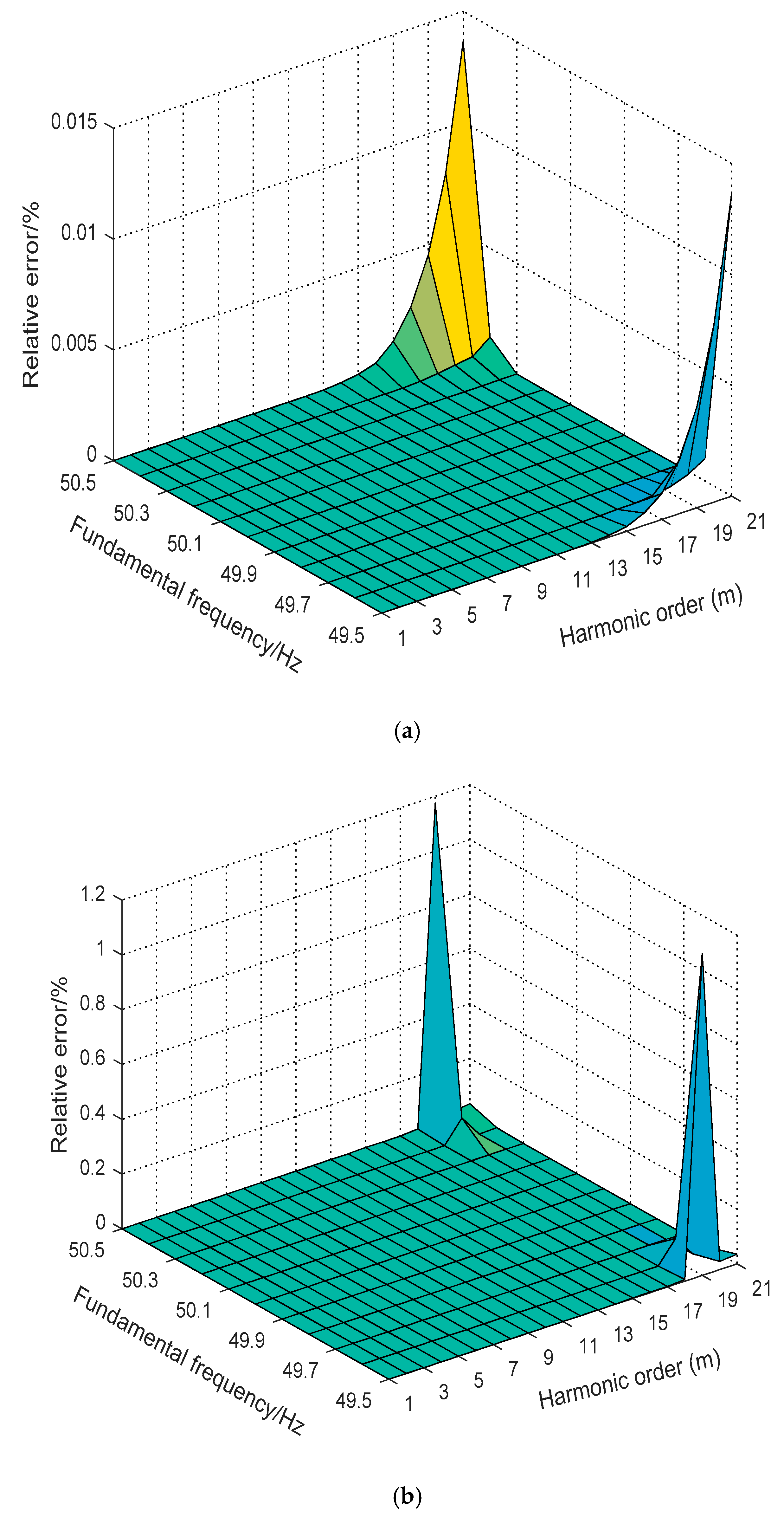
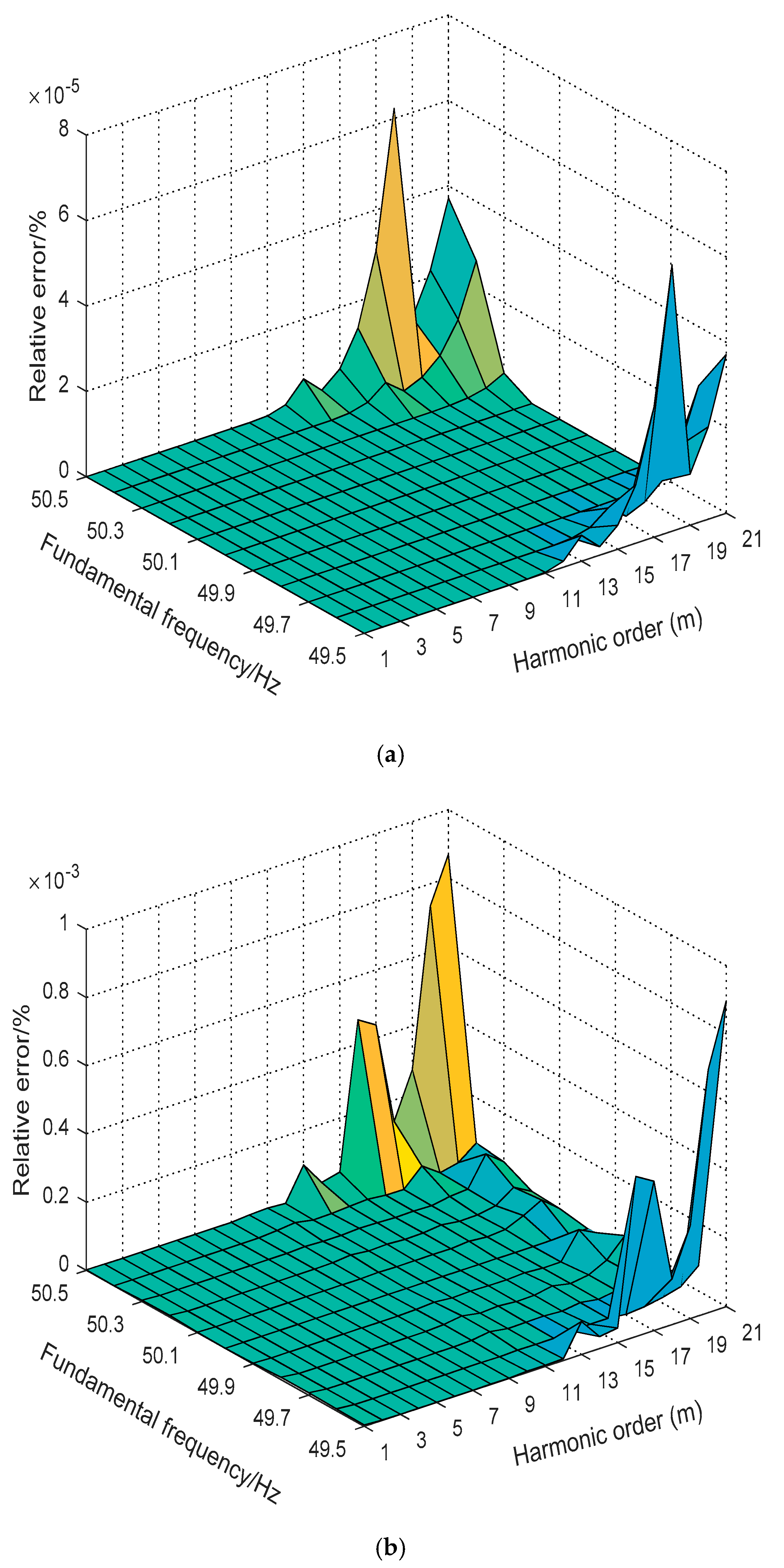
4.2. Detection of Harmonic Parameters in the Condition of Frequency Fluctuation

It is known that the fundamental frequency of the practical electricity grid is subject to fluctuation, which causes interference of the harmonics. This is more observable in the high-order and weak-amplitude harmonic signal that is easily affected by large-amplitude harmonics causing serious spectrum leakage in the condition of fundamental frequency fluctuation.

In order to validate the feasibility of the proposed six-term MSOW and the proposed improved algorithm in the condition of power frequency fluctuation, a simulation was carried out with a frequency fluctuation set to 49.5~50.5 Hz. The simulation signal adopts the preceding in Equation (26). In this simulation, the proposed improved six-term MSOW and the Nuttall window were adopted to calculate the measurement accuracy, in which the Nuttall window was used for comparison. Figure 5 shows the measurement error of the Nuttall window and Figure 6 depicts the measurement error of the proposed improved six-term MSOW.

As can be seen from Figure 5, when the fundamental frequency fluctuates between 49.5 and 50.5 Hz, the amplitude and phase measurement errors of the Nuttall window increase dramatically, especially for the high-order and weak-amplitude harmonics. In such case, the relative error of the amplitude is 10⁻²% and the relative error of the phase is 1.2%, which will not meet the requirements of the harmonic measurement standard of an electricity grid [25]. As can be seen from Figure 6, when the frequency fluctuates to 45.5~45.6 or 50.4~50.5 Hz, the measurement error of the amplitude and phase of high-order harmonics increases but can still meet the requirements of harmonic measurement standard. On the other hand, when the frequency fluctuates to 45.7~50.3 Hz, the measurement error of harmonic parameters is quite small which can also meet the requirements of the harmonic measurement standard.

In conclusion, simulation results reveal the improved performance of the proposed six-term MSOW and the proposed improved algorithm when the frequency fluctuates around the power frequency from 49.5 to 50.5 Hz. As shown in Figure 6, the measurement error of the amplitude and phase parameters are about 10⁻⁵% and 10⁻³%, respectively, which meet the requirement of the harmonic measurement in a practical power grid.

5. Experiment Analysis

In the practical power gird, the harmonic detection is influenced by many factors. Therefore, it is meaningful and significant to carry out an experiment test, in order to validate the practical application of the proposed six-term MSOW and the improved DFT harmonic detection algorithm. In the experiment, the conventional Blackman–Harris window was used for comparison.

In this experiment, the harmonic detection system consisted of a standard power source FLUKE6105A and a signal capture card. The signal with fundamental and harmonic components was generated from the FLUKE6105A standard power source, and the signal capture card was used for signal acquisition. The fundamental frequency of the signal was set to 50.1 Hz, and the number of sampling points was 1024. In the test results, the harmonic parameters set by the standard power source are regarded as true values, and the value measured by the DFT harmonic algorithm is regarded as the measurement value. Comparing the measurement value and the true value, the amplitude parameter is set as relative error, and the phase parameter is set as absolute error for which the unit is set as minute for apparent comparison. Only the results of the first to the seventh harmonic measurements are presented in

Table 7. Experiment measurement results.

Window Function	Harmonic Order	1	2	3	4	5	6	7
Blackman–Harris	Amplitude relative error/%	0.012	0.032	0.030	0.078	0.016	0.092	0.060
	Phase error/’	2.1	3.6	5.2	15.1	10.5	14.7	14.0
6-term MSOW	Amplitude relative error/%	0.003	0.018	0.004	0.010	0.005	0.005	0.004
	Phase error/’	1.8	2.2	4.1	14.0	9.8	13.6	13.8

.

It can be seen from the data in Table 7 that the proposed six-term MSOW is more accurate than the conventional Blackman–Harris window in terms of amplitude parameter and phase parameter measurement. In particular, for the measurement of the amplitude parameter, the maximum relative error of the six-term MSOW was 0.018%, while the Blackman–Harris window had a maximum measurement error of 0.092%. For the measurement of the phase parameter, the maximum error of the six-term MSOW was 14.0’, while that of the Blackman–Harris window was 15.1’. In conclusion, the experiment test verified that the proposed six-term MSOW and the improved DFT harmonic detection algorithm had improved performance in terms of harmonic detection in practical application.

6. Conclusions

In this paper, the constraints of minimizing the minimum side-lobe optimization window are established by optimizing the parameters of the combined cosine window. According to the optimizing process, a minimum aide-lobe optimization window is derived and proposed to reduce the influence of the spectrum leakage. In addition, an improved DFT harmonic detection algorithm based on the six-term minimum side-lobe optimization window and the four-spectrum-line interpolation method is proposed to improve the harmonic measurement accuracy for harmonic signal with high-order and weak-amplitude components, and when the power frequency fluctuates within a small range. Theoretical analysis, numerical simulation, and experiment test reveal that:

(1)

The proposed minimum side-lobe optimization window has the smallest side-lobe value compared with the cosine windows with the same terms. Besides, the proposed six-term minimum side-lobe optimization window has the smallest side-lobe peak compared with the existing conventional windows, which can effectively suppress the interaction of spectrum leakage and improve the measurement accuracy of the DFT harmonic detection method.

(2)

The simulation under complex harmonic condition proves that the proposed minimum side-lobe optimization window and the proposed improved DFT harmonic detection algorithm for harmonic analysis in an electricity grid exhibit higher measurement accuracy, can resist the influence of frequency fluctuation of the electricity grids, and can meet the standards of harmonic measurement under complex conditions.

With the wide application of nonlinear loads in the power grid, the issue of harmonic pollution caused by nonlinear loads has attracted the attention of researchers, and harmonic detection is the first step for harmonic research and harmonic elimination. Therefore, the measurement of harmonic parameters is of great significance for ensuring the safe and stable operation of the power grid, power quality evaluation, and power measurement. The existing windows and spectrum-line interpolation methods have a limitation in measuring the harmonic contents of a signal with high-order and weak-amplitude components when the power frequency fluctuates within a small range. Thus, the proposal of the MSOW and its practical application in harmonic detection is significantly crucial in power girds.

Theoretical analysis, simulation, and experiment test have shown that the proposed MSOW and the improved DFT algorithm based on six-term MSOW and four-spectrum-line interpolation method have improved performance to analyze harmonics in an electricity grid. Employing the proposed improved DFT algorithm, higher measurement accuracy can be achieved, and the influence of frequency fluctuation of the electricity grids can be reduced greatly. Thus, the issue of harmonic pollution in practical application of power girds caused by nonlinear loads can be greatly improved or ameliorated, and the power quality and power energy loss caused by the inaccurate harmonic detection can be strongly reduced or decreased.

References

1. Taskovski, D.; Koleva, L. Measurement of harmonics in power systems using near perfect reconstruction filter banks. IEEE Trans. Power Deliv. 2012, 27, 1025–1026. [Google Scholar] [CrossRef]
2. Nguyen, A.; Bui, V.; Hussain, A.; Nguyen, D.; Kim, H. Impact of demand response programs on optimal operation of multi-microgrid system. Energies 2018, 11, 1452. [Google Scholar] [CrossRef]
3. Li, Z.; Tao, Y.; Abu-Siada, A.; Masoum, M.A.S.; Li, Z.; Xu, Y. A new vibration testing platform for electronic current transformers. IEEE Trans. Instrum. Meas. 2019, 68, 704–712. [Google Scholar] [CrossRef]
4. López-Martín, V.M.; Azcondo, F.J.; Pigazo, A. Power quality enhancement in residential smart grids through power factor correction stages. IEEE Trans. Ind. Electron. 2018, 65, 8553–8564. [Google Scholar] [CrossRef]
5. Mcbee, K.D.; Simoes, M.G. Evaluating the long-term impact of a continuously increasing harmonic demand on feeder-level voltage distortion. IEEE Trans. Ind. Appl. 2014, 50, 2142–2149. [Google Scholar] [CrossRef]
6. Yang, N.; Huang, Y.; Hou, D.; Liu, S.; Ye, D.; Dong, B.; Fan, Y. Adaptive nonparametric kernel density estimation approach for joint probability density function modeling of multiple wind farms. Energies 2019, 12, 1356. [Google Scholar] [CrossRef]
7. Wu, Z.; Jiang, B.; Kao, Y. Finite-time H∞ filtering for Itô stochastic Markovian jump systems with distributed time-varying delays based on optimisation algorithm. IET Control Theory Appl. 2019, 13, 702–710. [Google Scholar] [CrossRef]
8. Reljin, I.S.; Reljin, B.D.; Papic, V.D. Extremely flat-top windows for harmonic analysis. IEEE Trans. Instrum. Meas. 2007, 56, 1025–1041. [Google Scholar] [CrossRef]
9. Orallo, C.M.; Carugati, I.; Maestri, S.; Donato, P.G.; Carrica, D.; Benedetti, M. Harmonics measurement with a modulated sliding Discrete Fourier Transform algorithm. IEEE Trans. Instrum. Meas. 2014, 63, 781–793. [Google Scholar] [CrossRef]
10. Jin, T.; Chen, Y.; Flesch, R.C.C. A novel power harmonic analysis method based on Nuttall-Kaiser combination window double spectrum interpolated FFT algorithm. J. Electr. Eng. 2017, 68. [Google Scholar] [CrossRef]
11. Ree, D.L.; Centeno, V.C.; Thorp, J.S.; Phadke, A.G. Synchronized phasor measurement applications power systems. IEEE Trans. Smart Grid 2010, 25, 20–27. [Google Scholar] [CrossRef]
12. Radil, T.; Ramos, P.M.; Serra, A.C. Spectrum leakage correction algorithm for frequency estimation of power system signals. IEEE Trans. Instrum. Meas. 2009, 58, 1670–1679. [Google Scholar] [CrossRef]
13. Barros, J.; Diego, R.I. On the use of the Hamming window for harmonic analysis the standard frame-work. IEEE Trans. Power Deliv. 2006, 21, 538–539. [Google Scholar] [CrossRef]
14. Lin, H.C.; Liu, L.Y. DFT-based recursive group-harmonic energy distribution approach for power interharmonic identification. Comput. Math. Appl. 2012, 64, 1128–1139. [Google Scholar] [CrossRef] [Green Version]
15. Jain, V.K.; Collins, W.L.; Davis, D.C. High accuracy analog measurements via interpolated FFT. IEEE Trans. Instrum. Means. 1979, 28, 113–122. [Google Scholar] [CrossRef]
16. Zhang, F.; Geng, Z.; Yuan, W. The algorithm of interpolating windowed FFT for harmonic analysis of electric power system. IEEE Trans. Power Deliv. 2001, 16, 160–164. [Google Scholar] [CrossRef]
17. Li, Y.; Zhao, T.; Wang, P.; Gooi, H.B.; Wu, L.; Liu, Y.; Ye, J. Optimal operation of multimicrogrids via cooperative energy and reserve scheduling. IEEE Trans. Ind. Inf. 2018, 14, 3459–3468. [Google Scholar] [CrossRef]
18. Duda, K. DFT Interpolation algorithm for Kaiser-Bessel and Dolph-Chebyshev windows. IEEE Trans. Instrum. Meas. 2011, 2, 784–790. [Google Scholar] [CrossRef]
19. Testa, A.; Gallo, D.; Langella, R. On the processing of harmonics and interharmonics: Using Hanning window in standard framework. IEEE Trans. Power Deliv. 2004, 19, 28–34. [Google Scholar] [CrossRef]
20. Harris, F.J. On the use of windows for harmonic analysis with the discrete Fourier transform. Proc. IEEE 1978, 66, 51–83. [Google Scholar] [CrossRef]
21. Qian, H.; Zhao, R.; Chen, T. Interharmonics analysis based on interpolating windowed FFT algorithm. IEEE Trans. Power Deliver. 2007, 22, 1064–1069. [Google Scholar] [CrossRef]
22. Wen, H.; Meng, Z.; Guo, S.; Li, F.; Yang, Y. Harmonic estimation using symmetrical interpolation FFT based on triangular self-convolution window. IEEE Trans. Ind. Inform. 2014, 11, 16–26. [Google Scholar] [CrossRef]
23. Qiu, L.; Li, Y.; Abu-Siada, A.; Xiong, Q.; Li, X.; Li, L.; Su, P.; Cao, Q. Electromagnetic force distribution and deformation homogeneity of electromagnetic tube expansion with a new concave coil structure. IEEE Access 2019. [Google Scholar] [CrossRef]
24. Su, T.; Yang, M.; Hussain, A.; Jin, T.; Flesch, R.C.C. Power harmonic and interharmonic detection method in renewable power based on Nuttall double-window all-phase FFT algorithm. IET Renew. Power Gener. 2018, 12, 953–961. [Google Scholar] [CrossRef]
25. Electromagnetic Compatibility (EMC)—Testing and Measurement Techniques—General Guide on Harmonics and Interharmonics Measurements and Instrumentation, for Power Supply Systems and Equipment Connected Thereto. Available online: https://infostore.saiglobal.com/store/PreviewDoc.aspx?saleItemID=2393892 (accessed on 8 May 2019).
Figure 1. Characteristic of the minimum side-lobe optimization window. (a) Time domain characteristic and (b) frequency domain characteristic.
Energies 12 02619 g001
Figure 2. Comparison of the spectrum characteristics between windows. (a) Comparison between the six-term MSOW and the six-term conventional window and (b) comparison between the six-term MSOW and the existing conventional windows.
Energies 12 02619 g002
Figure 3. Schematic diagram of harmonic signal spectrum.
Energies 12 02619 g003
Figure 4. Flow chart of the proposed improved discrete Fourier transform (DFT) harmonic detection algorithm.
Energies 12 02619 g004
Figure 5. Measurement error of the Nuttall window. (a) Amplitude relative error and (b) phase relative error.
Energies 12 02619 g005
Figure 6. Measurement error of the six-term MSOW. (a) Amplitude relative error and (b) phase relative error.
Energies 12 02619 g006